HAL Id: hal-00317993
https://hal.archives-ouvertes.fr/hal-00317993
Submitted on 19 May 2006
HAL is a multi-disciplinary open access
archive for the deposit and dissemination of
sci-entific research documents, whether they are
pub-lished or not. The documents may come from
teaching and research institutions in France or
abroad, or from public or private research centers.
L’archive ouverte pluridisciplinaire HAL, est
destinée au dépôt et à la diffusion de documents
scientifiques de niveau recherche, publiés ou non,
émanant des établissements d’enseignement et de
recherche français ou étrangers, des laboratoires
publics ou privés.
around the ionospheric hmF2
L. Liu, W. Wan, B. Ning
To cite this version:
L. Liu, W. Wan, B. Ning. A study of the ionogram derived effective scale height around the ionospheric
hmF2. Annales Geophysicae, European Geosciences Union, 2006, 24 (3), pp.851-860. �hal-00317993�
Ann. Geophys., 24, 851–860, 2006 www.ann-geophys.net/24/851/2006/ © European Geosciences Union 2006
Annales
Geophysicae
A study of the ionogram derived effective scale height around the
ionospheric hmF2
L. Liu, W. Wan, and B. Ning
Institute of Geology and Geophysics, Chinese Academy of Sciences, Beijing 100029, China
Received: 19 August 2005 – Revised: 9 February 2004 – Accepted: 23 February 2006 – Published: 19 May 2006
Abstract. The diurnal, seasonal, and solar activity vari-ations of the ionogram derived scale height around the ionospheric F-layer peak (H m) are statistically analyzed at
Wuhan (114.4◦E, 30.6◦N) and the yearly variations of H m
are also investigated for Wuhan and 12 other stations where
H mdata are available. H m, as a measure of the slope of the
topside electron number density profiles, is calculated from the bottomside electron density profiles derived from verti-cal sounding ionograms using the UMLCAR SAO-Explorer. Results indicate that the value of median H m increases with increasing solar flux. H m is highest in summer and lowest in winter during the daytime, while it exhibits a much smaller seasonal variation at night. A common feature presented at these 13 stations is that H m undergoes a yearly annual vari-ation with a maximum in summer during the daytime. The annual variation becomes much weaker or disappears from late night to pre-sunrise. In addition, a moderate positive correlation is found between H m with hmF2 and a strong correlation between the bottomside thickness parameter B0 and H m. The latter provides a new and convenient way for empirical modeling the topside ionospheric shape only from the established B0 parameter set.
Keywords. Ionosphere (Modeling and forecasting; Solar ra-diation and cosmic ray effects; General or miscellaneous)
1 Introduction
Knowledge of the spatial distribution of the electron den-sity in the ionosphere, especially the ionospheric profile
Ne(h), is important for scientific interest, such as
iono-spheric empirical modelings and ionoiono-spheric studies, and for practical applications for time delay correction of the radio wave propagation through the ionosphere, etc. Dur-ing the past decades, great efforts have been made in the
Correspondence to: L. Liu
global ionospheric empirical modeling (Bilitza, 2001). Many mathematical functions, such as the Chapman, exponen-tial, parabolic, Epstein functions, have been proposed to de-scribe the ionospheric profiles (e.g. Booker, 1977; Rawer et al., 1985; Rawer, 1988; Di Giovanni and Radicella, 1990; Stankov et al., 2003). Among these functions, the Chapman function is simple and has great potential for analytical mod-eling of the ionospheric profile (e.g. Huang and Reinisch, 2001). A nice feature of the Chapman profiler is that it only needs information about the electron density and height of the F peak and scale height to give a good representation
for the observed topside Ne(h). Studies have identified that
the Chapman function, even with a constant scale height, fits the topside ionospheric profile well several hundred kilome-ters above the F2-peak (Reinisch and Huang, 2004; Bele-haki et al., 2003). This is enough for most situations because most electrons in the ionosphere are distributed in this re-gion. When the scale height is linearly varied with height, the fit will be greatly improved in the higher region (Lei et al., 2005).
It is evident that the scale height is a key and inherent pa-rameter for ionospheric profiles, especially for the topside profiler (Stankov et al., 2003; Belehaki et al., 2006). How-ever, there are still limited studies on the behavior of the plasma scale height. Recently, Huang and Reinisch (2001) introduced a new technique to extrapolate the topside iono-sphere based on information from ground-based ionogram
measurements. They approximated the Ne(h) both around
and above the F2-layer peak (hmF2) by an α-Chapman func-tion with a scale height (H m) determined at hmF2. The parameter H m derived from ionograms is a measure of the electron density profile slope of the topside ionosphere. The
H mdata is routinely archived at some stations after being
derived from the Digisonde ionograms with the UMLCAR SAO-Explorer (http://ulcar.uml.edu/).
In this paper, we conduct a statistical analysis on the variations of the ionogram derived scale height (H m) around the F2-peak during 1999–2004 from routine
0 12 24 36 48 60 72 0 25 50 75 100 Year: 2004 Doy: 301−303 F107=127.8 ΣKp = 6.3 F107=131.6 ΣKp = 4.3 F107=127 ΣKp = 12 UT (hour) Hm (km) Kp 0 12 24 36 48 60 72 0 25 50 75 100 Year: 2003 Doy: 302−304 F107=275.4 ΣKp = 58.3 F107=267.6 ΣKp = 56 F107=245.2 ΣKp = 50.3 UT (hour) Hm (km) Kp
Fig. 1. Diurnal variations of the scale height (H m) derived from Digisonde measurements recorded at Wuhan during 29–31 October 2003
and 27–29 October 2004. The median values of H m in the nearest 31 days are plotted in dashed lines for a reference. The 3-hour Kpindex
is illustrated in the histograms. The corresponding daily sum Kpand solar index F107 indices are also labeled. Local Time, LT, is UT plus
7.6 h at Wuhan.
Digisonde measurements recorded at Wuhan (geographic
114.4◦E, 30.6◦N; 45.2◦ dip), China, and on the yearly
variations of H m observed at Wuhan, College (64.9◦N,
212.2◦E), Narssarssuaq (61.2◦N, 314.6◦E), Chilton
(51.6◦N, 358.7◦E), Millstone Hill (42.6◦N, 288.5◦E),
Tortosa (40.4◦N, 0.3◦E), Athens (38◦N, 23.5◦E), Wallops
Is. (37.8◦N, 284.5◦E), Ascension Is. (7.9◦S, 345.6◦E),
Madimbo (22.4◦S, 30.9◦E), Louisvale (28.5◦S, 21.2◦E),
Grahamstown (33.3◦S, 26.5◦E) and Port Stanley (51.7◦S,
302.2◦E) stations. The results will have empirical modeling
applications.
2 Data
The present analysis uses a database of H m observed at Wuhan, College, Narssarssuaq, Chilton, Millstone Hill, Tor-tosa, Athens, Wallops Is., Ascension Is., Madimbo,
Louis-vale, Grahamstown and Port Stanley. To investigate the
annual variation, H m data at the latter 12 stations were downloaded from the SPIDR web (http://spidr.ngdc.noaa. gov/spidr/).
More than 219 000 ionograms were routinely recorded at Wuhan (China) with a DGS-256 Digisonde during 1999– 2004. A huge effort has been made to manually scale those
ionograms, and the bottomside profiles are calculated from these hand-scaling ionograms with a standard “true height” inversion program (Reinisch and Huang, 1983; Huang and Reinisch, 1996) inherent in the UMLCAR SAO-Explorer. The critical frequency (foF2) and its height (hmF2) of the F-layer, the IRI bottomside profile thickness parameter B0, etc., are obtained. At the same time, the scale height around the F2-peak (H m) is also derived. The calculation of H m from the bottomside profile can be found in the work of Huang and Reinisch (2001) and Reinisch and Huang (2004). B0 is a bottomside thickness parameter that gives the height differ-ence between hmF2 and the height where the electron density profile has dropped down to 0.24*NmF2.
3 Results and discussions
3.1 Daily variation and geomagnetic dependence of Wuhan
H m
There are appreciable diurnal and day-to-day variations in the ionogram derived scale height around the F2-peak,
H m, derived from Digisonde measurements. Figure 1
dis-plays H m recorded at Wuhan for three geomagnetically disturbed days (29–31 October 2003) and three quiet days
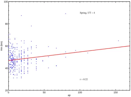
L. Liu et al.: An investigation of ionospheric effective scale height 853 0 50 100 150 20 40 60 80 100 r = 0.22 ap Hm (km) Spring, UT = 4
Fig. 2. Scatterplot of the scale height (H m) at Wuhan versus the 3-h geomagnetic activity index ap at 04:00 UT (around local noon) in
spring. The solid line shows the trend of the linear regression.
(27–29 October 2004). The median values of H m in the nearest 31 days are also plotted with dashed lines which serve as a reference level.
H mfor those three quiet days (27–29 October 2004) in
general follows the average behavior. In contrast, for three geomagnetically disturbed days (29–31 October 2003), the variability of H m is enhanced and it significantly deviated from the median behavior. This indicates the redistribution of the ionospheric ionization during geomagnetic disturbances due to the storm impact. Thus, for constructing a complete ionospheric image during storms, H m may present comple-mentary characteristics of the ionosphere.
The effects of geomagnetic storms on the ionosphere are well-known to be complicated and stochastic. The geomag-netic dependence of H m at Wuhan has been statistically in-vestigated with the planetary geomagnetic indices, 3-hour
Kp and Ap, and the daily Kp and Ap. Although H m may
greatly deviate from the average pattern under individual dis-turbed situations, the correlations of H m with these indices are poor, as depicted in Fig. 2. It implies a complicated de-pendence of H m on geomagnetic activity. Furthermore, it also suggests insignificant differences in the averaged values of H m at specified times for those 6 years if we separate
the data into two groups, low (Ap<15) and moderate to high
(Ap>15) magnetic activity levels.
3.2 Seasonal and solar activity variations of Wuhan H m
Several atmospheric and ionospheric parameters display reg-ular seasonal and solar activity variations (e.g. Richards, 2001; Lei et al., 2005). At low and middle latitudes, the pri-mary source of ionization in the F-region is the EUV solar
irradiances. The solar activity dependence of ionospheric characteristics has been studied in the early various iono-spheric observations. Richards et al. (1994) have shown that the solar cycle variation of most solar EUV flux lines can be scaled accurately enough for aeronomic applications by us-ing F107p = (F107 + F107A)/2, where F107A is the 81-day running mean of daily F107 index. Now we use F107p as an indicator of the solar activity level in this analysis.
Figure 3 presents the mothly diurnal variation of H m at Wuhan in 2002. The average and day-to-day variability of the monthly H m is described by the corresponding median and upper and lower quartiles, which are represented in lines with vertical bars, respectively. It can be observed from the figure that the values of median H m vary from 30–80 km. As seen from Fig. 3, H m are roughly of a similar behavior in the months from November to February. It is true for H m grouped in March and April, May to August, and Septem-ber and OctoSeptem-ber, respectively. Thus, to look for their sea-sonal variation, the parameters in months from November to February are classified as winter, March and April as spring, May to August as summer, and September and October as autumn, respectively.
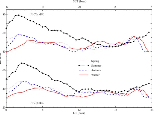
Diurnal variations of the median H m for four seasons un-der high (F107p>180) and moun-derate-to-low (F107p<140) solar activity levels are plotted in Fig. 4. In Fig. 4, data are grouped according to their solar activity levels. The possible influence of geomagnetic activities is not excluded.
Under moderate-to-low and high solar activities, a morn-ing increase in H m is followed by an afternoon decrease. There is no significant change in H m during the nighttime compared with the daytime, except for a small peak in the
winter under high solar activity. In summer, H m has a
0 50 Hm (km) January 0 50 Hm (km) February 0 50 Hm (km) March 0 50 Hm (km) April 0 50 Hm (km) May 0 50 Hm (km) June 0 50 Hm (km) July 0 50 Hm (km) August 0 50 Hm (km) September 0 50 Hm (km) October 0 6 12 18 24 0 50 UT (hour) Hm (km) November 0 6 12 18 24 0 50 UT (hour) Hm (km) December Year: 2002
Fig. 3. Diurnal variations of H m at Wuhan in 2002. Lines with bars, respectively, represent the monthly median values of H m and the
corresponding upper and lower quartiles. The local noon and local night are also indicated with open and solid circles near the abscissa, respectively. 0 6 12 18 24 20 40 60 40 60 80 UT (hour) Hm (km) Winter Autumn Summer Spring F107p<140 F107p>180 8 14 20 2 8 SLT (hour)
Fig. 4. Diurnal variations of H m for seasons under high (F107p>180) and moderate-to-low (F107p<140) solar activity levels. Here the
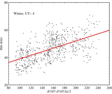
L. Liu et al.: An investigation of ionospheric effective scale height 855 80 100 120 140 160 180 200 220 240 260 20 40 60 80 (F107+F107A)/2 Hm (km) Winter, UT= 4
Fig. 5. Scatterplot of the scale height H m versus the solar activity index F107p at 04:00 UT in winter. The solid line shows the trend of the
linear regression. 0 6 12 18 24 0 0.1 0.2 0.3 UT (hour) dHm/dF107p (km) Winter Autumn Summer Spring
Fig. 6. Diurnal variations of the rate of H m increase with F107p in four seasons. Here the solar proxy is F107p = (F107+F107A)/2, where
F107A is the 81-day running mean of the daily F107 index.
notable diurnal variation with a maximum around 10:00 LT
and a minimum around midnight. Both under high and
moderate-to-low solar activity, H m is at its minimum dur-ing nighttime. The winter peak of H m shifts to local midday under high solar activity and even later under moderate-to-low solar activity. The diurnal variation of seasonal median
H mis not so appreciable in other seasons as that in summer.
An evident feature found in Figs. 3 and 4 is that the mean
daytime values of H m are highest in summer and lowest in winter, while insignificant seasonal differences are seen in the nighttime H m. During the daytime, the observed H m values in summer are about 20 km larger than those in other seasons.
According to Huang and Reinisch (2001), there is a good correlation between H m and the slab thickness of the iono-sphere, which is defined by the ratio of ionospheric total
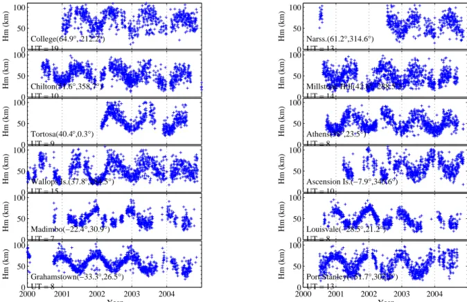
0 50 100 College(64.9°, 212.2°) UT = 19 Hm (km) 0 50 100 Narss.(61.2°,314.6°) UT = 13 Hm (km) 0 50 100 Chilton(51.6°,358.7°) UT = 10 Hm (km) 0 50 100 Millstone Hill(42.6°, 288.5°) UT = 14 Hm (km) 0 50 100 Tortosa(40.4°,0.3°) UT = 9 Hm (km) 0 50 100 Athens(38°,23.5°) UT = 8 Hm (km) 0 50 100 Wallops Is.(37.8°,284.5°) UT = 15 Hm (km) 0 50 100 Ascension Is.(−7.9°,345.6°) UT = 10 Hm (km) 0 50 100 Madimbo(−22.4°,30.9°) UT = 7 Hm (km) 0 50 100 Louisvale(−28.5°,21.2°) UT = 8 Hm (km) 20000 2001 2002 2003 2004 50 100 Grahamstown(−33.3°,26.5°) UT = 8 Hm (km) Year 20000 2001 2002 2003 2004 50 100 Port Stanley(−51.7°,302.2°) UT = 13 Hm (km) Year
Fig. 7. Time sequences of values of scale height (H m) at hmF2 over 12 stations at specified day times during 2000–2004. The names and
their locations of the stations are labeled.
electron content to the peak density. The seasonal feature of Wuhan H m is also similar to the general trend for the slab thickness to decrease from summer to equinox to win-ter as reported by Goodwin et al. (1995), Jayachandran et al. (2004) and Wu et al. (1998).
It is evident that the solar activity level should have an in-fluence on H m. Figure 5 gives a scatterplot of Wuhan H m versus F107p at 04:00 UT in winter. Although the data set has not covered a full solar cycle, the solar activity index F107 during the observations extends from the minimum of 80 to the maximum of 285.5 (on 28 September 2001), with a mean value of 157. In order to study the solar activity variations of H m, we investigate the relationship between
H mand F107p at each specified time for the four seasons.
It dindicates that the overall trend of the H m change is a linear increase with respect to F107p, namely the values of
H mtend to be higher for higher solar activities. Thus, the
solar dependence of H m may be represented with the rate of increase with solar flux, dH m/dF107p. Figure 6 demon-strates dH m/dF107p against universal time for the four sea-sons. The value of dH m/dF107p averages at 0.13 km per solar flux unit by day and night.
If the scale height in an α-Chapman function represents the scale height of the neutral atmosphere, the plasma scale height should be roughly twice as large as the Reinisch
and Huang (2004) method. The neutral temperature Tn at Wuhan, provided by the MSIS model (Picone et al., 2002), is shown in the fifth panel of Fig. 8. It is obvious that H m is not strongly connected with T n. It is also true for electron or ion temperatures, because there is a significant morning rise in electron and ion temperatures in the F-layer (Oyama et al., 1996; Sharma et al., 2005), while it does not occur in H m.
It should be mentioned that the classical scale height is de-fined as kT /mg (here k is the Boltzmann constant, T is the temperature, m is the mass and g the gravitation accelera-tion), while the scale height H m, derived from ionograms, is actually a measure of the slope of the topside electron num-ber density profile with a Chapman function, thus it does have not the classical physical meanings. This point has been made by Huang and Reinisch (2001). But H m derived from the ionograms has some physical meanings. First, the
iono-gram derived H m is a measure of the Ne(h)profile, thus it
may be thought of as an index for the slope of the topside
ionosphere. It has values in topside Ne(h)modeling
applica-tions. Second, this H m is also a measure of slab thickness, although their values may be different from each other, ac-cording to the statistical study of Huang and Reinisch (2001) on NmF2, TEC and H m. In addition, although the Chap-man theory can only be applied in the E- and F1-layer, the distribution of the electron density of the topside ionosphere
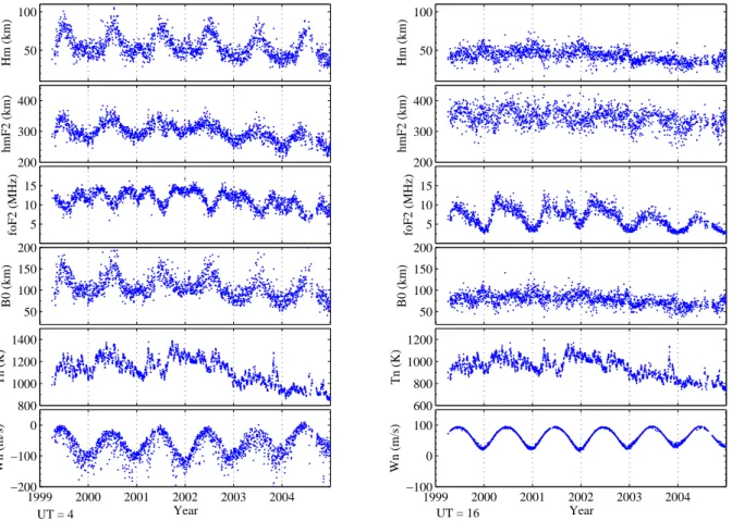
L. Liu et al.: An investigation of ionospheric effective scale height 857 50 100 Hm (km) 50 100 Hm (km) 200 300 400 hmF2 (km) 200 300 400 hmF2 (km) 5 10 15 foF2 (MHz) 5 10 15 foF2 (MHz) 50 100 150 200 B0 (km) 50 100 150 200 B0 (km) 800 1000 1200 1400 Tn (K) 600 800 1000 1200 Tn (K) 1999 2000 2001 2002 2003 2004 −200 −100 0 Year Wn (m/s) 1999 2000 2001 2002 2003 2004 −100 0 100 Year Wn (m/s) UT = 4 UT = 16
Fig. 8. Time sequences of values of scale height H m, foF2, hmF2, B0, thermospheric temperature T n (at the height of hmF2 from MSIS
model), and southward neutral wind W n (at the height of hmF2 from HWM model) over Wuhan at 04:00 UT (left) and 16:00 UT(right) during 1999–2004.
not far away from the F-layer peak can be well described by the Chapman function. Thus, the ionogram derived H m should contain information on the ionospheric chemical and dynamic processes. This point deserves further investigation.
3.3 Annual variation of H m at 13 stations
The Earth’s ionosphere is known to undergo a yearly varia-tion (e.g. Kawamura et al., 2002; Yu et al., 2004). It is well known that in some parts of the world the predominant vari-ation of foF2 is semiannual, but elsewhere it is significantly annual, usually with a winter maximum (e.g. Torr and Torr, 1973; Yu et al., 2004). To investigate the yearly variation of
H m, besides Wuhan, data at College, Narssarssuaq, Chilton,
Millstone Hill, Tortosa, Athens, Wallops Is., Ascension Is., Madimbo, Louisvale, Grahamstown and Port Stanley were also collected. H m data at these 12 ionosonde stations can be available on the SPIDR web. The latitude of these stations
varies from 64.9◦N to 51.7◦S.
An interesting feature of daytime H m, which occurs at all latitudes, is its significant annual variation with a sum-mer maximum. Figure 7 shows the time sequence of the
day-by-day H m at a specific time during the daytime over these global 12 stations. During the daytime, the annual com-ponent is dominant in the yearly variation of H m.
We choose the Wuhan station as an example to show the yearly variation of H m and hmF2, foF2 and the IRI bottom-side profile thickness parameter B0. Figure 8 shows the day-by-day values of these parameters over Wuhan around lo-cal noon and midnight, respectively. The yearly variation of
H mat Wuhan also shows the common feature at the other
12 stations. In addition, H m has a similar phase with that of
hmF2 and B0 and an opposite one with foF2. At midnight,
the yearly variation of hmF2 and B0 becomes much weaker and tends to disappear. In contrast, the annual variation of
foF2 is predominant with a peak in summer.
Figure 9 illustrates the amplitudes of the annual and semi-annual components of H m, hmF2, foF2 and B0 at Wuhan at different times, while Figure 10 represents the annual phase of these parameters at Wuhan. The yearly variation of Wuhan
foF2 has notable annual and semiannual components,
al-though its daytime annual phase is in winter, while at night, its annual variation is predominant with a peak in summer. In contrast, the behaviors of H m, hmF2 and B0 are somewhat
8 14 20 2 8 10 20 Ai (Hm) (km) SLT (hour) 20 40 Ai (hmF2) (km) 1 2 3 Ai (foF2) (MHz) 6 12 18 24 0 20 40 UT (hour) Ai (B0) (km) Annaul Semiannual
Fig. 9. Amplitudes of annual and semiannual components of H m, foF2, hmF2 and B0 at Wuhan in 2000–2001.
8 14 20 0 8 3 6 9 12 φ (Hm) SLT (hour) 3 6 9 12 φ (hmF2) 3 6 9 12 φ (foF2) 0 6 12 18 24 3 6 9 12 UT (hour) φ (B0)
Fig. 10. Phase of the annual component of H m, foF2, hmF2 and B0 at Wuhan in 2000–2001. The phases are in months.
different from that of foF2. Their annual phases are in sum-mer (Fig. 10). As shown in Fig. 9, daytime H m and hmF2 at Wuhan undergo a strong yearly variation with a predomi-nant annual component, while at night the yearly variations become much weaker and tend to disappear. Both the annual and semiannual components of H m and B0 become insignif-icant at night.
3.4 The correlation between H m and hmF2, B0
Scatterplots of the scale height H m versus hmF2, foF2 and B0 at Wuhan at local noon (04:00 UT) and midnight (16:00 UT) during 1999–2004 are given in the left and right panels of Fig. 11, respectively. In general, H m (also B0) shows a moderate positive correlation with hmF2 and a very weak negative or poor correlation with foF2.
A striking feature shown in Fig. 11 is the strong correlation between H m and the IRI bottomside thickness parameter B0 at all local times over Wuhan (with a correlation coefficient as high as 0.92–0.99). Both parameters B0 and H m are de-pendent on the shape of the electron density profile in the F region. This dependence justifies the strong correlation be-tween both parameters. Reinisch et al. (2004) discussed the possibility to calculate H m from the IRI parameters B0, B1 and D1. Their ultimate purpose is searching for an alternate path to an estimate of the topside profile based on the bot-tomside one. Our result suggests that the strong correlation between H m and B0 provides a new and convenient way for future modeling of the topside ionospheric shape only from the established B0 parameter set. This point may be helpful for improving the IRI profile prediction in the future.
L. Liu et al.: An investigation of ionospheric effective scale height 859 200 300 400 r = 0.68 hmF2 (km) 200 300 400 r = 0.65 hmF2 (km) 5 10 15 r = −0.43 foF2 (MHz) 5 10 15 r = −0.01 foF2 (MHz) 20 40 60 80 100 50 100 150 200 r = 0.93 B0 (km) Hm (km) 20 40 60 80 100 50 100 150 200 r = 0.97 B0 (km) Hm (km) UT = 4 UT = 16
Fig. 11. Scatterplot of the scale height H m versus hmF2, foF2, and IRI thickness parameter B0 at Wuhan around local noon (left, at
04:00 UT) and midnight (right, 16:00 UT) during 1999–2004.
The positive correlation of H m with hmF2 suggests that the physical processes involved in controlling the variation of hmF2 may also be responsible for that of H m. That hmF2 greatly depends on the direct effect of horizontal neutral wind is well known from the past and well explained by the the-ory of the thermospheric winds. Neutral winds and electric fields act to shift the F peak from the balance height to a new level. It is the physical basis of deriving the meridional neu-tral wind from ionospheric observations (e.g. Rishbeth et al., 1978; Buonsanto et al., 1997; Liu et al., 2003, 2004). The annual variation arises from the summer to winter thermo-spheric circulation wind. The meridional neutral wind (Wn) for Wuhan around hmF2 obtained by the HWM93 model (Hedin et al., 1996) is illustrated in the bottom panel of Fig. 8. As expected, during daytime, the model Wn shows a similar annual pattern as that of hmF2 and H m. It indicates that Wn not only contributes to the ionospheric height but also to the shape of the ionospheric profile. At night, the model Wn still has a significant annual variation, which is far from that of
H m. This point deserves further study, although the current
version of the HWM93 model has its limitations.
4 Summary
This paper investigates the diurnal, seasonal, and solar ac-tivity variations of the ionogram derived scale height around
hmF2 observed at Wuhan and the yearly variations of H m at
Wuhan and 12 other stations. The main results are summa-rized as follows:
(1) It shows that H m observed at Wuhan has appreciable diurnal and day-to-day variations. Significant distur-bances in H m are presented during geomagnetic active periods. However, the dependence of H m on magnetic activity is complicated.
(2) The diurnal behaviors of seasonal median H m under both solar activities are found to be similar. Median val-ues of H m are highest in summer and lowest in winter during the daytime. At nighttime, H m exhibits a much weaker seasonal variation. H m tends to a higher value with increasing solar flux.
(3) A distinct annual variation of H m is observed at Wuhan and 12 other stations, i.e. H m has a higher value in sum-mer and a lower value in winter during the daytime. This annual variation becomes much weaker or disap-pears at the time interval from late night to pre-sunrise. (4) A strong correlation is found between H m and the bot-tomside thickness parameter B0 at all local times. It provides a new and convenient way for modeling the topside ionospheric shape only from the established B0 parameter set. In general, H m shows a moderate posi-tive correlation with hmF2 and negaposi-tive and little corre-lation with foF2 depending on the local time.
Acknowledgements. The authors thank two referees for their
valu-able suggestions for improving the presentation of the paper. The SAO-Explorer software is provided by UMass Lowell Center for Atmospheric Research. The data at global 12 ionosonde stations are downloaded from the Space Physics Interactive Data Resource (SPIDR) web (http://spidr.ngdc.noaa.gov/spidr/). This research was supported by the KIP Pilot Project (kzcx3-sw-144) of Chinese Academy of Sciences and National Natural Science Foundation of China (40574071, 40574072) and National Important Basic Re-search Project (G2000078407). The author (L. Liu) gratefully ac-knowledges the support of K. C. Wong Education Foundation, Hong Kong.
Topical Editor M. Pinnock thanks two referees for their help in evaluating this paper.
References
Belehaki, A., Jakowski, N., and Reinisch, B.: Comparison of iono-spheric ionization measurements over Athens over Athens us-ing ground ionosonde and GPS derived TEC values, Radio Sci., 38(6), 1105, doi:10.1029/2003RS002868, 2003.
Belehaki, A., Marinov, P., Kutiev, I., Jakowski, N., and Stankov, S.: Comparison of the topside ionosphere scale height determined by topside sounders model and bottomside digisonde profiles, Adv. Space Res., doi:10.1016/j.asr.2005.09.015, in press, 2006. Bilitza, D.: International reference ionosphere 2000, Radio Sci.,
36(2), 261–275, 2001.
Booker, H. G.: Fitting of multi-region ionospheric profiles of elec-tron density by a single analytic function of height, J. Atmos. Terr. Phys., 39, 619–623, 1977.
Buonsanto, M. J., Starks, M. J., Titheridge, J. E., Richards, P. G., and Miller, K. L.: Comparison of techniques for derivation of neutral meridional winds from ionospheric data, J. Geophys. Res., 102, 14 477–14 484, 1997.
Di Giovanni, G. and Radicella, S. M.: An analytical model of the electron density profile in the ionosphere, Adv. Space Res., 10(11), 27–30, 1990.
Goodwin, G. L., Silby, J. H., Lynn, K. J. W., Breed, A. M., and Es-sex, E. A.: GPS satellite measurements: ionospheric slab thick-ness and total electron content, J. Atmos. Terr. Phys., 57(14), 1723–1732, 1995.
Hedin, A. E., Fleming, E. L., Manson, A. H., et al.: Empirical wind model for the upper, middle and lower atmosphere, J. Atmos. Terr. Phys., 58(13), 1421–1447, 1996.
Huang, X. and Reinisch, B. W.: Vertical electron profiles from the Digisonde network, Adv. Space Res., 18(6), 121–129, 1996. Huang X. and Reinisch, B. W.: Vertical electron content from
iono-grams in real time, Radio Sci., 36(2), 335–342, 2001.
Jayachandran, B., Krishnankutty, T. N., and Gulyaeva, T. L.: Clima-tology of ionospheric slab thickness, Ann. Geophys., 22, 25–33, 2004.
Kawamura, S., Balan, N., Otsuka, Y., and Fukao, S.: An-nual and semianAn-nual variations of the midlatitude iono-sphere under low solar activity, J. Geophys. Res., 107(A8), doi:10.1029/2001JA000267, 2002.
Lei, J., Liu, L., Wan, W., and Zhang, S.-R.: Variations of elec-tron density based on long-term incoherent scatter radar and ionosonde measurements over Millstone Hill, Radio Sci., 40, RS2008, doi:10.1029/2004RS003106, 2005.
Liu, L., Luan, X., Wan, W., Ning, B., and Lei, J.: A new approach to the derivation of dynamic information from ionosonde mea-surements, Ann. Geophys., 21(11), 2185–2191, 2003.
Liu, L., Luan, X., Wan, W., Lei, J., and Ning, B.: Solar activity vari-ations of equivalent winds derived from global ionosonde data, J. Geophys. Res., 109, doi:10.1029/2004JA010574, 2004. Oyama, K.-I., Watanabe, S., Su, Y., Takahashi, T., and Hiro, K.:
Seasonal, local time, and longitudinal variations of electron tem-perature at the height of ∼600 km in the low latitude region, Adv. Space Res., 18(6), 269–278, 1996.
Picone, J. M., Hedin, A. E., Drob, D. P., and Aikin, A. C.: NRLMSISE-00 empirical model of the atmosphere: Statistical comparisons and scientific issues, J. Geophys. Res., 107(A12), 1468, doi:10.1029/2002JA009430, 2002.
Rawer, K.: Synthesis of ionospheric electron density profiles with Epstein functions, Adv. Space Res., 8(4), 191–198, 1988. Rawer, K., Bilitza, D., and Gulyaeva, T. L.: New formulas for IRI
electron density profile in the topside and middle ionosphere. Adv. Space Res., 5(7), 3–12, 1985.
Reinisch, B. W. and Huang, X.: Automatic calculation of electron density profiles from digital ionograms: 3. Processing of bottom-side ionograms, Radio Sci., 18(3), 477–492, 1983.
Reinisch, B. W. and Huang, X.: Deducing topside profiles and total electron content from bottomside ionograms, Adv. Space Res., 27(1), 23–30, 2004.
Reinisch, B. W., Huang, X., Belehaki, A., Shi, J., Zhang, M., and Ilma, R.: Modeling the IRI topside profile using scale height from ground-based ionosonde measurements, Adv. Space Res., 34, 2026–2031, 2004.
Richards, P. G., Fennelly, J. A., and Torr, D. G.: EUVAC: A solar EUV flux model for aeronomic calculations, J. Geophys. Res., 99(A5), 8981–8992, 1994.
Richards, P. G.: Seasonal and solar cycle variations of the iono-spheric peak electron density: comparison of measurement and models, J. Geophys. Res., 106(A12), 12 803–12 819, 2001. Rishbeth, H., Ganguly, S., and Walker, J. C. G.: Field-aligned and
field-perpendicular velocities in the ionospheric F2 layer, J. At-mos. Terr. Phys., 40, 767–784, 1978.
Sharma, D. K., Rai, J., Israil, M., and Subrahmanyam, P.: Diurnal, seasonal and longitudinal variations of ionospheric temperatures of the topside F region over the Indian region during solar min-imum (1995–1996), J. Atmos. Solar-Terr. Phys., 67, 269–274, 2005.
Stankov, S. M., Jakowski, N., Heise, S., Muhtarov, P., Ku-tiev, I., and Warnant, R.: A new method for reconstruction of the vertical electron density distribution in the upper iono-sphere and plasmaiono-sphere, J. Geophys. Res., 108(A5), 1164, doi:10.1029/2002JA009570, 2003.
Torr, M. R. and Torr, D. G.: The seasonal behaviour of the F2-layer of the ionosphere, J. Atmos. Terr. Phys., 35, 2237–2251, 1973. Wu, J., Long, Q., and Quan, K.: A statistical study and modling of
the ionospheric TEC and the slab thickness with observations at Xinxiang, China, Chinese J. Radio Sci., 13(3), 291–296, 1998. Yu, T., Wan, W., Liu, L., and Zhao, B.: Global scale annual and
semi-annual variations of daytime NmF2 in the high solar activ-ity years, J. Atmos. Solar-Terr. Phys., 66, 1691–1701, 2004.