HAL Id: hal-00317799
https://hal.archives-ouvertes.fr/hal-00317799
Submitted on 22 Dec 2004
HAL is a multi-disciplinary open access
archive for the deposit and dissemination of
sci-entific research documents, whether they are
pub-lished or not. The documents may come from
teaching and research institutions in France or
abroad, or from public or private research centers.
L’archive ouverte pluridisciplinaire HAL, est
destinée au dépôt et à la diffusion de documents
scientifiques de niveau recherche, publiés ou non,
émanant des établissements d’enseignement et de
recherche français ou étrangers, des laboratoires
publics ou privés.
interplanetary coronal mass ejections
M. Owens, P. Cargill
To cite this version:
M. Owens, P. Cargill. Non-radial solar wind flows induced by the motion of interplanetary coronal
mass ejections. Annales Geophysicae, European Geosciences Union, 2004, 22 (12), pp.4397-4406.
�hal-00317799�
Annales Geophysicae (2004) 22: 4397–4406 SRef-ID: 1432-0576/ag/2004-22-4397 © European Geosciences Union 2004
Annales
Geophysicae
Non-radial solar wind flows induced by the motion of interplanetary
coronal mass ejections
M. Owens1,*and P. Cargill1
1Space and Atmospheric Physics, The Blackett Laboratory Imperial College, London SW7 2BW, UK *now at: Center for Space Physics Boston University, Boston MA 02215, USA
Received: 22 December 2003 – Revised: 28 August 2004 – Accepted: 3 September 2004 – Published: 22 December 2004
Abstract. A survey of the non-radial flows (NRFs)
dur-ing nearly five years of interplanetary observations revealed the average non-radial speed of the solar wind flows to be ∼30 km/s, with approximately one-half of the large (>100 km/s) NRFs associated with ICMEs. Conversely, the average non-radial flow speed upstream of all ICMEs is
∼100 km/s, with just over one-third preceded by large NRFs. These upstream flow deflections are analysed in the context of the large-scale structure of the driving ICME. We chose 5 magnetic clouds with relatively uncomplicated upstream flow deflections. Using variance analysis it was possible to infer the local axis orientation, and to qualitatively estimate the point of interception of the spacecraft with the ICME. For all 5 events the observed upstream flows were in agreement with the point of interception predicted by variance analysis. Thus we conclude that the upstream flow deflections in these events are in accord with the current concept of the large-scale structure of an ICME: a curved axial loop connected to the Sun, bounded by a curved (though not necessarily circu-lar) cross section.
Key words. Interplanetary physics (flare and stream
dynam-ics; interplanetary magnetic fields; interplanetary shocks)
1 Introduction
It is well known that interplanetary coronal mass ejections (ICMEs) undergo a significant interaction with the solar wind during their transit from the Sun to the Earth. The most obvi-ous manifestation of this is their tendency to be decelerated or accelerated towards the speed of the ambient solar wind (e.g. Gopalswamy et al., 2000, 2001; Vrˇsnak and Gopal-swamy, 2002; Owens and Cargill, 2004). While the interac-tion between an ICME and the solar wind can be described in terms of an aerodynamic drag force and associated drag
coef-Correspondence to: M. Owens
(mjowens@bu.edu)
ficient (e.g. Cargill et al., 1995, 1996; Vrˇsnak, 2001; Cargill, 2004), this in fact involves a number of complex stages.
When the ICME speed exceeds the relevant magnetohy-drodynamic wave speed (usually the fast mode) a collision-less bow shock forms in front of the ICME that deceler-ates, compresses and heats the solar wind plasma. Behind this shock there is a sheath region of dense hot plasma and magnetic field that may be compressed and/or draped around the ICME. Indeed, magnetic field draping ahead of ICMEs has been directly observed in the outer heliosphere (McCo-mas et al., 1988, 1989; Jones et al., 2002). The sheath is also where the shocked solar wind flow must be deflected around the ICME. The need for deflection arises from the fact that the solar wind plasma and field are frozen together, and thus cannot penetrate into the ICME. This is particularly clear for the case of magnetic clouds (e.g. Burlaga, 1988), where the ICME is treated as a large flux rope. Early work by Gosling et al. (1987) detected westward flow deflections with a typical magnitude of ∼25 km/s and they concluded that ICMEs are systematically deflected eastward by the mag-netic stresses of the Parker-spiral IMF acting on the west flank of ICMEs.
The magnitude and especially the direction of flow deflec-tions measured by a spacecraft will depend on which part of the ICME the spacecraft encounters. This point will be expanded on in Sect. 3, but can be introduced here by con-sidering a case where the ICME is a magnetic flux rope. The leading surface of such a flux rope has two radii of curvature: one due to the rooting of its footpoints at the Sun (axial cur-vature), and one due to its finite cross section (cross-sectional curvature). Since one would expect the deflected flows to be locally approximately parallel to the surface, the properties of the measured flows must reflect the ICME geometry.
It is thus clear that the detection of these deflected flows, and in particular a determination of their direction relative to the surface of the ICME, is an important diagnostic of the interaction between ICMEs and the solar wind. This paper presents an investigation of such flow deflections. In Sect. 2 we present a survey of non-radial flows in the solar wind at
50 100 150 200 250 300 350 0 200 400 50 100 150 200 250 300 350 0 200 400 50 100 150 200 250 300 350 0 200 400
Non−radial flow speed (km/s)
50 100 150 200 250 300 350 0 200 400 50 100 150 200 250 300 350 0 200 400 Day of year 1998 1999 2001 2002 2000
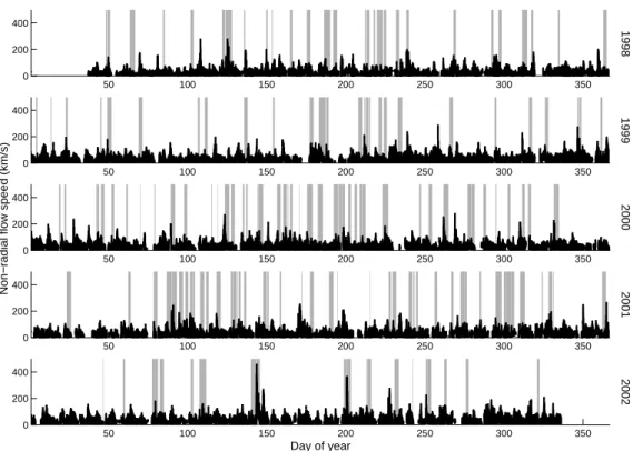
Fig. 1. The non-radial flow speed for 5 years of SWEPAM data. The grey shaded areas represent regions of solar wind identified as ICMEs
by Cane and Richardson (2003).
1 AU using several years of interplanetary data, and deter-mine what fraction can be associated with ICMEs. This pro-vides a broad overview of the occurrence of flow deflections. In Sect. 3 we discuss how the flow deflection depends on the curvature of the leading surface of the ICME and present an analysis technique that can determine the flow deflection in the context of the spacecraft location with respect to the ICME. Section 4 presents a number of case studies of flow deflections.
2 Survey of non-radial solar wind flows
We first examine the existence of non-radial flows in the so-lar wind at 1 AU. If the magnitude of non-radial flows asso-ciated with ICMEs exceeds that in the ambient solar wind, then such flows are likely to be a signature of ICME-induced flow deflections. Solar wind plasma data from the SWEPAM instrument (McComas et al., 1998) on the Advanced Com-position Explorer (ACE) spacecraft between 1 January 1998 and 31 December 2002 are used. We work in GSE coordi-nates, so that a radial ICME motion translates into motion in the −xGSE direction. We then define the non-radial (or transverse) flow speed (|Vt|)as V2t=V2Y+V
2
Z, where VY and VZare the components of the flow velocity in the yGSE and zGSEdirections, respectively. We note that the survey results are very similar if the angle between the velocity vector and the radial direction is used in place of the non-radial flow speed.
The solid black lines in Fig. 1 shows the 5-min averaged
|Vt| between 1998 and 2002. To establish the connection of |Vt|with ICMEs, we draw on the ICME survey of Cane and Richardson (2003). On the basis of magnetic field and plasma data, they identified 214 ICMEs at 1 AU in the pe-riod 1996–2002 from which we use the subset of 180 ICMEs observed in 1998–2002. Periods of solar wind identified as ICMEs are shown as the grey shaded areas in Fig. 1. One can see at a glance that there appears to be some overlap between high non-radial velocities and the presence of ICMEs.
Noting that the average magnitude of the non-radial flow velocity in the solar wind for the period considered was
∼30 km/s, we can make things more concrete and define a non-radial flow (NRF) as an interval of solar wind with
|Vt|>50 km/s. Multiple NRFs occurring within 12 h are pre-sumed to be driven by the same disturbance, and are treated as a single event. Figure 2a shows a histogram of the max-imum non-radial speed associated with all NRF events ob-served in the 5 years of SWEPAM data. The light shaded area indicates NRFs that occurred within 12 h of solar wind inter-vals identified as ICMEs by Cane and Richardson (2003), with the solid line showing the fraction (0 to 100% from top to bottom of plot) of NRFs in each speed bin associated with ICMEs. The dark shaded area and dashed line repre-sent a subset of fast ICMEs, defined as having average ra-dial speeds greater than 450 km/s. Approximately half of the larger (>100 km/s) non-radial flows are readily associated with ICMEs. Indeed, both of the largest NRFs (>300 km/s) are associated with fast ICMEs and from Fig. 1 appear to
M. Owens and P. Cargill: Non-radial solar wind flows induced by the motion of interplanetary coronal mass ejections 4399 0 100 200 300 400 500 0 50 100 150 200 250 300 (a) Maximum |V t| of NRF (km/s) Frequency 0 100 200 300 400 500 0 10 20 30 40 50 60 70 Max |V t| upstream of ICME (km/s) Frequency (b)
Fig. 2. Plot (a) shows a histogram of the maximum transverse flow
speed of non-radial flows (NRFs) observed by ACE. We define a NRF as a period of solar wind with |Vt|>50 km/s. The light (dark)
shaded area indicates NRFs that occurred within 12 h of solar wind intervals identified as (fast) ICMEs. The solid (dashed) line shows the percentage of NRFs in each speed bin associated with (fast) ICMEs. Plot (b) shows a histogram of the maximum transverse flows speeds upstream of ICMEs (dark regions indicate fast ICMEs, with the dashed line showing the percentage of all ICMEs that are fast). The upstream region is taken to be the 12-h period ahead of the ICME leading edge.
occur at the boundaries between multiple ICMEs.
However, it is also clear from Figs. 1 and 2a that not all ICMEs generate significant solar wind flow deflections, and conversely, not all large non-radial flows can be readily as-sociated with ICMEs. We thus took the identified ICMEs in the Cane and Richardson (2003) data set, and examined the magnitude of the upstream flow deflections. Here the upstream region is defined as the solar wind in the 12-h pe-riod preceding the ICME leading edge. For each ICME, the maximum non-radial flow speed in this upstream region was found and the results are shown in Fig. 2b. The light and dark shaded areas represent all and fast ICMEs, respectively, with the dashed line showing the fraction (0 to 100% from top to bottom of the plot) of ICMEs in that non-radial speed bin that are fast. The mean value of the maximum transverse flow speed preceding all (fast) ICMEs is 101.3 km/s (137.0 km/s), with 38% (65%) of all (fast) ICMEs exhibiting a maximum non-radial flow speed greater than 100 km/s in the upstream solar wind region.
It is well known that a non-radial component to the solar wind velocity can be generated at the interface of two inter-acting solar wind streams. However, at least during periods close to solar maximum, a significant fraction of the non-radial solar wind flows at 1 AU are associated with ICMEs. The deflection of the ambient solar wind by the transient ejecta suggests a means for estimating both part of the ICME encountered by the observing spacecraft, and the shape of the ICME leading edge. In the following section we outline a method for interpreting the upstream flow deflections in terms the large-scale structure of ICMEs.
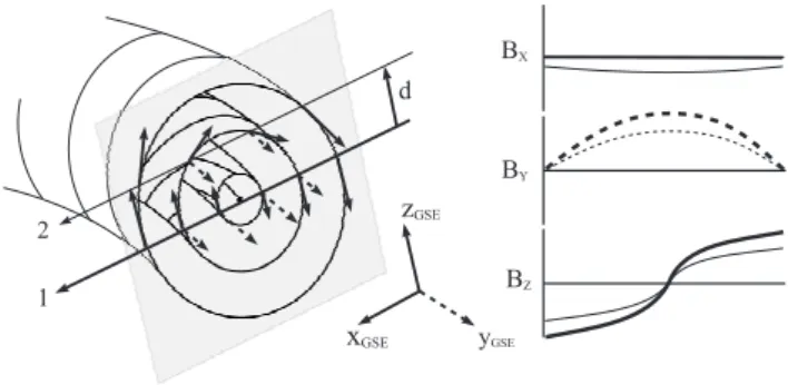
Fig. 3. A sketch of the geometry of an ICME. The local axis of
the magnetic cloud is in the yGSEdirection, and the circular
cross-section is in the xGSE–zGSE plane. Vectors perpendicular
(par-allel) to yGSE are shown as solid (dashed) lines. Two spacecraft trajectories through the flux-rope are shown, and sketches of the ob-served magnetic field parameters are shown on the right-hand side, with trajectory 1 (2) shown as the thick (thin) line.
3 Analysis of flow deflections
The results of Sect. 2 indicate the need to develop analysis methods to examine flow deflections at individual ICMEs. The magnitude and direction of the deflection must depend on the geometry of the leading surface of the ICME and we adopt the scenario that an ICME is a large magnetic flux rope, with both feet rooted in the solar surface (i.e. a mag-netic cloud). Then in the absence of magmag-netic reconnection between the ICME and solar wind magnetic fields (for details see Cargill et al., 1996), the leading surface of the ICME is a curved flux surface through which plasma does not pene-trate, implying a deflected flow parallel to this surface. The direction and magnitude of the deflected flow will depend on the orientation of the ICME surface and its speed relative to the solar wind.
The shape of this surface will be determined by two types of curvature: axial curvature due to the rooting of the foot-points of the ICME at the Sun and cross-sectional curvature due to its internal magnetic field structure. While each cur-vature is determined by different processes, there is some ev-idence that they have similar scales (Russell and Mulligan, 2002). An important issue is whether the local radii of curva-ture are the same at all points on the surface. Early work (e.g. Burlaga, 1988) suggested that magnetic clouds had a circular cross section, but more recent experimental and theoretical work indicates that ICMEs can be elongated considerably in a direction perpendicular to their direction of motion (Russell and Mulligan, 2002; Cargill and Schmidt, 2002). This non-uniformity of curvature can have important consequences.
As an example of the type of flow deflections expected, consider the schematic picture of a flux rope shown in Fig. 3. For simplicity we present the situation at the ICME nose where the flux rope axis and axial radius of curvature point in the yGSE and xGSE directions, respectively. Vectors per-pendicular (parallel) to yGSE are shown as solid (dashed) lines. If the spacecraft encounters the ICME at yGSE=0 and
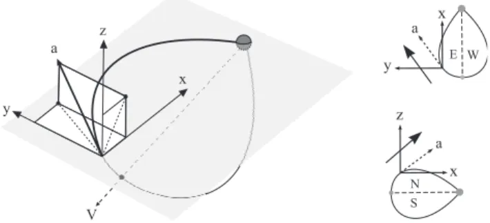
Fig. 4. An explanation of the axis projections in terms of the
large-scale orientation of magnetic clouds. The curved line represents a magnetic cloud axis, the dot represents the nose of the cloud (the effect of solar rotation has been ignored). The axis intersects the ecliptic plane (shown as the grey panel), where local axis orientation
(a) is the thick arrow. Projections of the axis onto the ecliptic and
xGSE–zGSEplanes are shown as dashed lines, and are interpreted
in terms of the ICME “flanks” in the two smaller diagrams on the right-hand side. By requiring the xGSEcomponent of the axis to be
positive, a positive (negative) yGSE indicates an intersection east (west) of the nose. Similarly, a positive (negative) zGSEindicates
an intersection north (south) of the nose.
a distance d above the zGSE=0 axis, the flow must be de-flected in the positive zGSE and xGSE directions. If d is then replaced by −d, the deflection in the zGSE direction is reversed. If the spacecraft is displaced in the yGSE direc-tion, but remains at zGSE=0, the deflection then acquires a component in the yGSE direction. Finally, a displacement away from both yGSE=0 and zGSE=0 leads to a general de-flected flow with components in all three directions. Thus, if one knows the (local) orientation of the flux rope axis, and whether one is above or below the mid-point of the ICME cross section, one can predict the direction of the non-radial flow. However, the magnitude and direction of the flow will also depend on the shape of the leading surface.
Turning first to the orientation of the ICME axis, this can be estimated using Minimum Variance Analysis (MVA, see Sonnerup and Cahill, 1967, for a general discussion and Bothmer and Schwenn, 1988, for application to ICMEs). For the case shown in Fig. 3, the maximum (emax), intermediate (eint), and minimum (emin)variance directions of the mag-netic field will be in the zGSE, yGSE and xGSE directions, respectively (Bothmer and Schwenn, 1998), subject to am-biguities discussed below. Note, in particular, that the axis orientation is determined by the intermediate variance direc-tion. Sketches of the magnetic field components for this ex-ample are shown on the right-hand side of Fig. 3 for a space-craft passing through the centre (thick lines) and a distance d above the axis (the thin lines).
There is a 180◦ambiguity in the variance directions and it is therefore necessary to impose additional constraints. We require eint to be parallel to the axial magnetic field (in this case to point in the positive yGSE direction) and the min-imum variance direction to have a positive xGSE compo-nent. Thus, the right-handed variance coordinate system
for the flux-rope shown in Fig. 3 would be (emax, eint, emin)=(−zGSE, yGSE, xGSE). In the variance coordinate system, the chirality of the magnetic cloud is defined by the sense of the rotation in the maximum variance magnetic field: the positive to negative rotation shown in the example indi-cates a left-handed rotation.
For “off-axis” crossings (trajectory 2 and thin lines in Fig. 3), the variance directions are not so well defined. This manifests itself in lower eigenvalue ratios, coupled with less recognisable signatures in the behaviour of the variance mag-netic field components (the thin lines in Fig. 3). Thus we couple the results of MVA with a visual inspection of the magnetic field hodograms, and some judgement is required to establish the viability of MVA. The error in the axis ori-entation estimated by variance analysis increases with the in-creasing closest approach distance of the spacecraft to the axis (|d|), but nominally this error is within 10◦(e.g. Burlaga and Behannon, 1982).
For crossings through the flux rope axis (yGSE=0 here), the magnetic field in the minimum variance direction (Bmin) is approximately zero. However, for off-axis crossings, Bmin6=0. This fact can be used to qualitatively infer the spacecraft position relative the axis (i.e. d in Fig. 3), using the handedness of the flux-rope and the polarity of the Bmin. For example, trajectory 2 in Fig. 3 sees a positive to nega-tive rotation in Bmax, indicating a left-handed flux-rope. It also measures a negative Bmin. One can then infer that the position of the spacecraft relative to the flux-rope axis (d), has a negative value of emax. We term this type of ICME en-counter as a “negative” crossing (conversely, a crossing at a position with a positive emaxcomponent would be termed a “positive” crossing). Note that as emax=−zGSEin this par-ticular case, the “negative” crossing actually translates to a spacecraft interception “above” the axis relative to the zGSE direction. However, it is logical to work in the variance coor-dinate system when defining the spacecraft crossing relative to the axis, as the axis may (in principle) have any orientation with respect to the GSE coordinate axes.
Based on the above discussion, we can write down gen-eral rules for the type of crossing. Defining the handed-ness (H) to be +(−)1 for right-(left-) handed flux ropes, the “crossing”, as defined above, is given by the sign of
−Hsgn(Bmin) where sgn(x) is 1(−1) for x>(<)0. The cross-ing location relative to the zGSE=0 axis is given by the sign of −Hsgn(Bmin)sgn(emax(ˆz)).
We proceed with the analysis of the flow deflection by defining a local axis vector ˆa to lie along eint, but to have a positive xGSE component (i.e. ˆa is either parallel or anti-parallel to eint: see Fig. 4 for a sketch). This defines ˆa to point in the direction of the flow deflection (in the ICME rest frame) resulting from axial curvature. The “flank” of the ejecta encountered by the spacecraft can be inferred from the axis vector if the ICME is assumed to have the form of a curved axial loop rooted at both ends to the Sun, as shown in Fig. 4. To enable an intercomparison of ICME encoun-ters, we classify ICMEs based upon axis projections onto the xGSE–yGSE and xGSE–zGSE planes. A positive (negative)
M. Owens and P. Cargill: Non-radial solar wind flows induced by the motion of interplanetary coronal mass ejections 4401 yGSE component indicates an intersection east (west) of the
nose. Similarly, a positive (negative) zGSEindicates an inter-section north (south) of the nose.
We now assume that the leading edge of the ICME is lo-cally planar. Thus, the normal to the local leading edge ( ˆn), the incoming flow velocity (directed along xGSE)and the di-rection of the deflected flow velocity (Vd)all lie in the same plane, such that: ˆVd= ˆn×(ˆxGSE× ˆn). For axial encounters (i.e. d=0), cross-sectional curvature can be ignored, and the normal to the leading edge is given by: ˆn= ˆa×( ˆa׈xGSE). Thus, for spacecraft trajectories intersecting the axis, flow deflections should be axis-aligned, as shown by the solid ar-rows in the right-hand side of Fig. 4. (When ˆa is perpendic-ular to xGSE, the direction of the deflected flow is undefined. This is the stagnation point at the nose of the ejecta.)
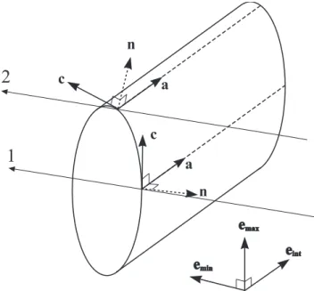
Conversely, without axial curvature (i.e. a nose encounter) the flow will be deflected around the cross section of the ICME, perpendicular to ˆa. We define a unit vector ˆc to lie in the plane of the leading edge, orthogonal to ˆa and to have a positive xGSE component (see Fig. 5). Furthermore, we require that ˆc has a positive (negative) emax component for “positive” (“negative”) spacecraft crossings, as defined above. Thus, ˆc points in the direction of the flow deflection resulting from cross-sectional curvature (see also Fig. 5). For spacecraft crossings near the nose of ejecta (where axial cur-vature can be ignored) the normal to the leading edge is given by: ˆn=ˆc×(ˆc׈xGSE). For spacecraft trajectories just above the axis relative to emax (i.e. the closest approach distance of the spacecraft to the axis is negligible), ˆc→emax, whereas
ˆ
c→eminfor trajectories clipping the outer edge (i.e. the clos-est approach distance of the spacecraft to the axis is compa-rable to the radius of the flux-rope), as shown in Fig. 5.
In general, both axial and cross-sectional effects are im-portant, so the normal to the leading edge is ˆn= ˆa׈c and the direction of the flow deflection can then be written as:
ˆ
Vd=(ˆa׈c)×[ˆxGSE×( ˆa׈c)]). Thus, the deflected flow di-rection always lies between the vectors ˆa and ˆc. Variance analysis can completely describe the axial vector ˆa. How-ever, without the use of a flux-rope model (and hence as-sumptions about the cross-sectional shape of ICMEs), we are unable to quantitatively estimate the closest approach dis-tance (d), and therefore are unable to completely describe ˆc. For “positive” (“negative”) axis crossings, our knowledge of
ˆ
c is limited to the fact that it must always lie between emax
and emin (−emax and emin). Hence, we know the orienta-tion of ˆc only to within 90◦. For a “positive” magnetic cloud encounter (i.e. above the axis relative to emax)the upstream flow deflection should lie between ˆa and emin, and have a positive emaxcomponent, whereas for “negative” crossings, Vd is again expected to lie between ˆa and emin, but with a negative emaxcomponent.
Finally, in order to apply the proposed analysis technique it is necessary to transform the measured velocities (i.e. in the spacecraft rest frame) into the rest-frame of the ICME, so that the solar wind flows toward the leading edge of the ICME in the positive xGSE direction. However, there often exist large velocity gradients through a radial cut of an ICME
Fig. 5. The normals to the leading edge of an ICME for different
closest approach distances of the spacecraft to the axis: trajectory 1 passes close to the axis, whereas trajectory 2 clips the outer edge of the ICME cross section. For trajectory 1, c→emax, resulting in
n→−emin. For trajectory 2, c→emin, resulting in n→emax.
owing to its expansion. Additionally, matters are compli-cated if the expansion of the ICME is not completely cylin-drically symmetric, meaning identification of the character-istic ICME speed, and hence performing the correct frame transformation, is non-trivial.
In this study we limit the analysis of the flow deflection to the non-radial components of the flow, avoiding the need for any transformation. This restricts comparison between the expected and observed flows to projections onto the non-radial (i.e. yGSE-zGSE)plane. In the case studies of Sect. 4, we use the angle between the upstream flow direction and the axis vector, defined by cos θ =|Vd·eint|/|eint||Vd|, where only the y and z components of the vectors are used. How-ever, the effect of projection must be taken into considera-tion. For spacecraft encounters through the ICME axis, Vdis expected to lie along the non-radial projection of ˆa, whereas for encounters at the very top or bottom edge of the ICME,
Vd should be aligned with the projection of emin. At inter-mediate distances from the axis, Vd should thus lie between the projections of ˆa and emin, with a positive (negative) emax component for “positive” (“negative”) spacecraft crossings. Thus, the position of the observed flow deflection between the two extremes allows for a first-order estimate of the dis-tance from the axis at which the spacecraft intercepts the ICME. To quantify this parameter we calculate the ratio of
θto the angle between the projections of ˆa and emin, the lat-ter angle measured so as to include a positive (negative) emax component for “positive” (“negative”) spacecraft crossings. The angle ratio is denoted θn, and is expected to have a value between 0 (for axis aligned flows) and 1 (for emin aligned flows).
Table 1. The five magnetic clouds with ordered non-radial flows in the upstream sheath region. The ICME number indicates the event
number in the Cane and Richardson (2003) ICME catalogue.
Event ICME number Year ICME Start (DOY) ICME End (DOY) Sheath start (DOY) Sheath end (DOY)
A 35 1998 63.62 65.08 63.45 63.6
B 57 1998 268.3 269.4 267.97 268.26
C 136 2000 277.65 279.0 277.01 277.42
D 154 2001 102.35 103.29 101.55 101.92
E 186 2001 304.87 306.34 304.54 304.82
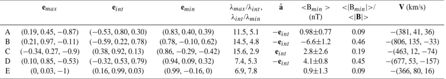
Table 2. Details of the flux-rope orientations and upstream flow deflections for the 5 case studies considered. Orientation parameters: the
three variance directions in (xGSE, yGSE, zGSE)format, maximum to intermediate and intermediate to minimum eigenvalue ratios, the
direction of the axis vector relative to eint, magnetic field strength in the emindirection (<Bmin>)and its fractional contribution to the total field strength (<|Bmin|>/<|B|>). The average flow in the upstream disturbance (V) is listed as (VX, VY, VZ), in GSE coordinates.
emax eint emin λmax/λint, aˆ <Bmin> <|Bmin|>/ V (km/s)
λint/λmin (nT) <|B|> A (0.19, 0.45, −0.87) (−0.53, 0.80, 0.30) (0.83, 0.40, 0.39) 11.5, 5.1 −eint 0.98±0.77 0.09 −(381, 41, 36) B (0.21, 0.97, −0.11) (−0.59, 0.22, 0.78) (0.78, −0.10, 0.62) 14.5, 4.8 −eint −6.6±1.2 0.46 −(806, 135, −33) C (−0.34, 0.27, −0.9) (0.38, 0.92, 0.13) (0.86, −0.29, −0.42) 15.6, 2.9 eint 2.8±2.6 0.19 −(463, 12, −74) D (0.10, 0.85, −0.53) (−0.32, 0.53, 0.79) (0.94, 0.09, 0.32) 7.4, 5.3 −eint 4.1±0.8 0.45 −(677, 53, −157) E (0, 0.03, −1) (0.16, 0.99, 0.03) (0.99, −0.16, 0) 6.9, 7.8 0.9±1.3 0.09 −(366, 80, 16)
4 Examples of ICME-related flow deflections
We now use the analysis developed in the previous section to compare the orientations of ICMEs with the associated flow deflections. This analysis is performed for five events, all ob-served with the ACE spacecraft, and documented in the Cane and Richardson (2003) catalogue. Of the 214 ICMEs listed in the catalogue, 54 are listed as “magnetic clouds”, how-ever 20 of these ICMEs occurred before ACE became oper-ational. For the remaining 34 magnetic clouds we performed variance analysis on ACE magnetic field data (Smith et al., 1998). The event boundaries listed in the ICME catalogue are used as a reference point, but we vary the interval con-sidered so as to obtain the required signatures in the variance directions, and to a lesser extent, maximise the eigenvalue ratios. It was possible to obtain satisfactory MVA axes ori-entations for 21 clouds using both a formal analysis and an inspection of the hodograms.
We next examined the flow deflections in the upstream solar wind for these events. For three events there was no identifiable disturbance, but in general the non-radial flow velocity in the sheath region ahead of the magnetic clouds was highly structured, containing discontinuities and gradual rotations. Thus, for the majority of the events it is not immediately clear how to define the deflected flow velocity. For this reason we restrict this study to events with a relatively constant non-radial flow velocity throughout the sheath. We identified 5 such events with sheath and ICME properties in Table 1.
The first example was of a fast magnetic cloud that oc-curred on day 63, 1998. Figure 6 shows ACE magnetic field and plasma observations of this event, with the magnetic field presented in the minimum, intermediate and maximum vari-ance directions, which are in turn listed in Table 2, along with the eigenvalue ratios. The disturbance onset and ICME start and end times are shown by the solid vertical lines. The MVA analysis gives the most significant results when the ICME boundaries are taken at day numbers 63.62 and 65.08.
Figure 7 shows the variance vectors and ˆa in a three-dimensional representation (upper left), and projected onto the three planes of the GSE coordinate system (remaining panels). The magnetic field shows the characteristic posi-tive to negaposi-tive profile of the maximum variance magnetic field of a left-handed flux-rope. The average value of the minimum variance magnetic field is <Bmin>=0.98±0.77 nT (Table 2). The fraction of the ICME magnetic field strength in the minimum variance direction (i.e. <|Bmin|>/<|B|>) is very small (0.09), suggesting a crossing close to the axis. The positive value of <Bmin>for a left-handed flux-rope in-dicates the spacecraft trajectory was a “positive” crossing, in that the point of closest approach of the spacecraft to the axis has a positive emax component, but with a crossing below the zGSE=0 plane. The spacecraft encountered the south and west flanks of the ICME, so that ˆa=−eint, as shown in Fig. 7. The maximum 5-min average non-radial flow speed is 55.3 km/s and occurs approximately 75% of the way into the sheath. We note that this maximum flow is fairly representative of the transverse flow velocity throughout
M. Owens and P. Cargill: Non-radial solar wind flows induced by the motion of interplanetary coronal mass ejections 4403 62.5 63 63.5 64 64.5 65 65.5 66 66.5 −10 0 10 Bmax 62.5 63 63.5 64 64.5 65 65.5 66 66.5 −20 0 20 Bint 62.5 63 63.5 64 64.5 65 65.5 66 66.5 −10 0 10 Bmin 62.5 63 63.5 64 64.5 65 65.5 66 66.5 −450 −400 −350 −300 −250 Vx (km/s) 62.5 63 63.5 64 64.5 65 65.5 66 66.5 −50 0 50 Vy (km/s) 62.5 63 63.5 64 64.5 65 65.5 66 66.5 −50 0 50 Vz (km/s) 62.50 63 63.5 64 64.5 65 65.5 66 66.5 20 40 Np (cm − 3)
Fig. 6. Event A, day 63 1998. Magnetic field data (magnetic field
in variance coordinates) is shown in the top 3 panels, ion data (VX, VY and VZcomponents of the proton velocity, and proton density)
are shown in the bottom 4 panels. The disturbance, ICME start and end times are shown by the solid vertical lines. There is a small non-radial flow in the sheath preceding the ICME.
the whole sheath region, wherein <VY>=−22.3 and
<VZ>=−31.4 km/s. The sheath velocity vector is shown in the final column of Table 2, and Fig. 7 shows the projections of the variance directions and upstream flow deflection onto the yGSE-zGSE plane. Both the maximum and average ob-served transverse velocities in the sheath region agree with the flows expected for this ICME orientation.
As noted in Sect. 3, the direction of the flow deflection is expected to lie between ˆa and emin. The “positive” crossing means that Vdshould also have a positive emaxcomponent, as is the case. The angle (θ ) between the maximum (average) deflected flow direction and the axis vector is 20.9◦(34.3◦). Correcting for projection (i.e. dividing by 203.8◦, the angle between ˆa and emin, and rotating through positive emax) gives θnof 0.10 and 0.17 for the maximum and average flow vectors, respectively. Thus, the close approach to the axis suggested by the small minimum variance magnetic field is supported by the small angle between the flow deflection and axis, as projected onto the non-radial plane.
−1 −0.5 0 0.5 1 −1 0 1 −1 −0.5 0 0.5 1 XGSE YGSE ZGSE 1 0.5 0 −0.5 −1 −1 −0.5 0 0.5 1 X GSE Y GSE −1 −0.5 0 0.5 1 −1 −0.5 0 0.5 1 Z GSE X GSE 1 0.5 0 −0.5 −1 −1 −0.5 0 0.5 1 Z GSE Y GSE min max int a max min int a min int max a max min int a Vmax Vmax <V> <V> (a) (b) (c)
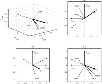
Fig. 7. The top left panel shows the axis orientation, variance
di-rections and flow deflections of event A. Plot (a) shows the projec-tions onto the ecliptic plane, plot (b) shows the projecprojec-tions onto the xGSE-zGSEplane. These projections should be compared to Fig. 4. The spacecraft encountered the south and west flanks of the ICME. Plot (c) shows flow deflections and variance directions of event A projected onto the non-radial (i.e. yGSE–zGSE)plane. Variance
di-rections are shown as dashed lines, the axis vector is the solid arrow. The maximum and average transverse sheath velocity unit vectors are shown as solid lines. The observed flow deflections are consis-tent with the “positive” crossing inferred by variance analysis (i.e. they both lie between the axis and minimum variance directions, rotating through positive emax).
The details of the remaining four events are summarised in Fig. 8 where the projection of the variance vectors and Vd on the y-z plane are shown, as well as in Tables 1 and 2. For each event, we find the following:
– Event B is a well-defined magnetic cloud and has a
pos-itive to negative rotation of Bmax, indicative of a left-handed rotation of the flux-rope magnetic field, and is a “negative” traversal. The minimum variance mag-netic field accounts for a significant fraction of the to-tal magnetic field of the ICME, suggesting that the dis-tance of closest approach to the axis was much larger than for event A. The spacecraft encountered the south and west flanks of the ICME so that ˆa=−eint. There is a large non-radial flow in the sheath region with a maximum 5-min averaged speed of 139 km/s, occurring 78% of the way through the sheath. The average non-radial flow components over the duration of the sheath are <VY>=−55.6 and <VZ>=−1.3 km/s. When the velocity and variance directions are projected onto the non-radial plane (Fig. 8, top left panel), the observed flow deflection falls within the range predicted by the orientation and point of interception of the magnetic cloud. The maximum (average) upstream flow makes an
−1 −0.5 0 0.5 1 ZGSE −1 −0.5 0 0.5 1 −1 −0.5 0 0.5 1 Y GSE −1 −0.5 0 0.5 1 min min min min max max max max int = int int int a Vmax <V> Vmax Vmax Vmax <V> <V> <V> a a Event B Event C Event D Event E ZGSE Y GSE
Fig. 8. The axis orientations, variance directions and flow
deflec-tions of events B, C, D and E, in the same format as Fig. 7c.
angle of 88.1◦(72.7◦)with the axis vector. Dividing by 106.4◦(the angle between ˆa and emin rotating through negative emax)gives θn values of 0.83 and 0.68 using maximum and average upstream flows, respectively. We note the larger angle between the axis and flow vector projections compared with event A. This is also consis-tent with the closest approach being quite distant from the axis.
– Event C has a smaller relative speed than in the
previ-ous two examples, and as a result the upstream distur-bance takes the form of a bow-wave that has not steep-ened into a shock front. Nevertheless, the same deflec-tion of flow should still occur at the leading edge. In the maximum variance direction, the magnetic field ro-tates smoothly from negative to positive values, indi-cating a right-handed flux-rope. In this case, ˆa=eint, meaning ACE encountered the north and east flanks of the magnetic cloud. The maximum non-radial flow speed in the sheath is 75.3 km/s, occurring 72% of the way through the sheath. The yGSE and zGSE veloc-ity components averaged over the sheath duration were
−15.4 and 34.1 km/s, respectively. The orientation of the ICME compared with the upstream flow deflection is shown in Fig. 8 (top right panel). The observed flow deflection projected onto the non-radial plane lies be-tween the axis and minimum variance direction, with a negative maximum variance component, consistent with the orientation and point of observation estimated by variance analysis. The value of θnfor the maximum (av-erage) upstream flow direction is 0.40 (0.47), suggest-ing a closest approach further from the axis than event A, but closer than event B. The fraction of the magnetic
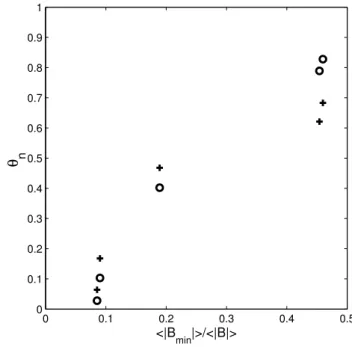
0 0.1 0.2 0.3 0.4 0.5 0 0.1 0.2 0.3 0.4 0.5 0.6 0.7 0.8 0.9 1 <|Bmin|>/<|B|> θ n
Fig. 9. The θnvalue (i.e. the “normalised” angle between the up-stream flow direction and axis vector) as a function of normalised magnetic field strength in the minimum variance direction, for the 5 events considered. Circles (crosses) show θncalculated from the
maximum (average) upstream flow direction.
field strength in the minimum variance direction agrees with this interpretation.
– Event D is an example with a strong non-radial flow
ahead of the fast moving magnetic cloud. It is also in-teresting to note the presence of a large amplitude but short duration NRF at the trailing edge of the mag-netic cloud, the result of a high speed stream behind the ICME. The flux-rope is right-handed, with a “neg-ative” spacecraft crossing. The axis vector, ˆa=−eint here, indicating a south and west flank encounter. Aver-aging over the entire sheath gives <VY>=−49.7 km/s and <VZ>=48.4 km/s. Again, we find the upstream flow deflections are as expected for the orientation of the ICME and point of observation of the spacecraft. The flow vector is closer to the minimum variance di-rection than the axis vector: θnfor the maximum (aver-age) upstream flow direction is 0.79 (0.62), suggesting the closest approach of the spacecraft was a significant distance from the magnetic cloud axis. This is in accord with the large magnetic field strength in the minimum variance direction.
– Event E has a clear non-radial flow in the sheath region,
flowed by a strong magnetic cloud signature. There is a SWEPAM data gap for much of the ICME body, but this does not affect our analysis of this event. Here the xGSE and zGSE components of the intermediate vari-ance direction are very small, resulting in undetermined flank encounters, and hence a 180◦ambiguity in the axis
M. Owens and P. Cargill: Non-radial solar wind flows induced by the motion of interplanetary coronal mass ejections 4405 vector. Examination of the magnetic field in the
maxi-mum variance direction reveals a left-handed flux-rope, and the small minimum variance field suggests a pos-sible “positive” spacecraft crossing, though the small value of <Bmin>is somewhat inconclusive. Thus, the point of interception of the spacecraft is likely to be close to the nose of the ejecta in both an axial and cross-sectional sense. In the sheath region, the maximum 5-min averaged transverse flow speed is 81.4 km/s, oc-curring 67% of the way through the sheath, and aver-aging over the whole sheath gives <VY>=−52.5 km/s and <VZ>=−24.0 km/s. Figure 8 (bottom right panel) shows the variance and the upstream flow directions projected onto the non-radial plane. The flow deflec-tion is in agreement with a spacecraft crossing above the axis. We do not show an axis vector due to the ambiguity in the ICME flank encountered. However, the flow deflection suggests ACE intercepted the ICME west of the nose. Assuming ˆa=−eint(i.e. the west flank crossing suggested by the flow direction), θn, using the maximum (average) Vd, is 0.03 (0.06), as expected for the small closest approach distance inferred by the neg-ligible magnetic field strength in the minimum variance direction.
These results are summarised in Fig. 9 which shows θn plotted as a function of the flux-rope magnetic field strength in the minimum variance direction for the 5 events consid-ered, with circles (crosses) showing θn calculated from the maximum (average) upstream flow direction. Both θn and
<|Bmin|>/<|B|> are expected to increase with increasing
distance from the axis of an ICME, though not necessarily linearly. These two independent methods of estimating the closest approach of the observing spacecraft to the axis of a magnetic cloud show good agreement. We also note that for these 5 events, the magnitude to the NRF speed in the sheath scales well with the ICME speed relative to the upstream so-lar wind.
5 Discussion and conclusions
This paper has addressed the plasma flows induced in the so-lar wind by the motion of ICMEs, in particuso-lar flows in the non-radial direction that must arise as fast-moving ICMEs push solar wind plasma aside. A survey of the non-radial flow speed in five years of solar wind data found approxi-mately half of the large NRFs to be associated with ICMEs. Fast ICMEs were shown to drive the strongest transverse solar wind flows. The direction of the non-radial deflec-tions was shown to be consistent with the local part of the ICME edge being encountered for five events studied in de-tail. However, it should be noted that the ordered flow deflec-tions required to perform such analysis are relatively rare.
For spacecraft interceptions through the axis of a mag-netic cloud, the minimum variance magmag-netic field should vanish. Furthermore, the upstream deflected flow should be axis aligned. As the closest approach distance between the
spacecraft and axis increases, the magnetic field strength in the minimum variance direction should increase, and the de-flected flow should rotate away from the axis toward the min-imum variance direction. The 5 events considered in this study were consistent with these general trends (as shown in Fig. 9), though further observations are required to quantify this effect. Upstream flow deflections (in conjunction with modelling of the flux-rope magnetic field) provide a possible means to infer the cross-sectional shape and extent of ejecta, and will form the basis of a future study.
Finally, we note the existence of significant non-radial flows in the body of ejecta, though the magnitude of such flows are nominally less than the preceding sheath region. Further study of the sense of these flows coupled with the ICME flank encountered is required to ascertain whether the systematic eastward deflection of ICMEs reported by Gosling et al. (1987) is present in the ACE data set.
Acknowledgements. M. Owens thanks PPARC and QuintiQ for
fi-nancial support. We have benefited from the availability of ACE data at NSSDC, in particular the MAG (N. Ness) and SWEPAM (D. McComas) instruments. We would also like to thank A. Rees for useful discussions.
The Editor in Chief thanks B. Vrˇsnak for his help in evaluating this paper.
References
Bothmer, V. and Schwenn, R.: The structure and origin of magnetic clouds in the solar wind, Ann. Geophys., 16, 1, 1998.
Burlaga, L. F.: Magnetic clouds: Constant alpha force-free config-urations, J. Geophys. Res., 93, 7217–, 1988.
Burlaga, L. F. and Behannon, K. W.: Magnetic clouds: Voyager observations between 2 and 4 AU, Sol. Phys., 81, 181, 1982. Cane, H. V. and Richardson I. G.: Interplanetary coronal mass
ejec-tions in the near-Earth solar wind during 1996–2002, J. Geophys. Res., 108, 1156, 2003.
Cargill, P. J.: On the Aerodynamic Drag Force Acting on Coronal Mass Ejections, Solar Phys., 221, 135, 2004.
Cargill, P. J. and Schmidt, J. M.: Modelling interplanetary CMEs using magnetohydrodynamic simulations, Ann. Geophys., 20, 879, 2002.
Cargill, P. J., Chen, J., Spicer, D. S., and Zalesak, S. T.: Geometry of interplanetary magnetic clouds, Geophys. Res. Lett., 22, 647, 1995.
Cargill, P. J., Chen, J., Spicer, D. S., and Zalesak, S. T.: MHD simulations of the motion of magnetic flux tubes through a mag-netized plasma, J. Geophys. Res., 101, 4855, 1996.
Gopalswamy, N., Lara, A., Lepping, R. P., Kaiser, M. L., Berdichevsky, D., and St. Cyr, O. C.: Interplanetary acceleration of coronal mass ejections, Geophys. Res. Lett., 27, 145, 2000. Gopalswamy, N., Lara, A., Yashiro, S., Kaiser, M. L., and Howard,
R. A.: Predicting the 1-AU arrival times of coronal mass ejec-tions, J. Geophys. Res., 106, 29 207, 2001.
Gosling, J. T., Thomsen, M. F., Bame, S. J., and Zwickl, R. D.: The eastward deflection of fast coronal mass ejecta in interplanetary space, J. Geophys. Res., 92, 12 399, 1987.
Jones, G. H., Rees, A., Balogh, A., and Forsyth, R. J.: The draping of heliospheric magnetic fields upstream of coronal mass ejecta, Geophys. Res. Lett., 29, 1520, 2002.
McComas, D. J., Gosling, J. T., Winterhalter, D., and Smith, E. J.: Interplanetary magnetic field draping about fast coronal mass ejections in the outer heliosphere, J. Geophys. Res. , 93, 2519, 1988.
McComas, D. J., Gosling, J. T., Bame, S. J., Smith, E. J., and Cane, H. V.: A test of magnetic field draping induced Bzperturbations
ahead of fast coronal mass ejecta, J. Geophys. Res., 94, 1465, 1989.
McComas, D. J., Bame, S. J., Barker S. J., Feldman, W. C., Phillips, J. L., Riley, P., and Griffee, J. W.: Solar wind electron proton alpha monitor (SWEPAM) for the Advanced Composition Ex-plorer, Space Sci. Rev., 86, 563, 1998.
Owens, M. J. and Cargill, P. J.: Predictions of the arrival time of Coronal Mass Ejections at 1 AU: An analysis of the causes of errors, Ann. Geophys., 22, 661, 2004.
Russell, C. T. and Mulligan, T.: On the magnetosheath thicknesses of interplanetary coronal mass ejections, Planet. Space Sci., 50, 527, 2002.
Smith, C. W., L’Heureux, J., Ness, N. F., Acuna, M. H., Burlaga, L. F., and Scheifele, J.: The ACE magnetic fields experiment, Space Sci. Rev., 86, 613, 1998.
Sonnerup, B. U. O. and Cahill, L. J.: Magnetopause structure and attitude from Explorer 12 observations, J. Geophys. Res., 72, 171, 1967.
Vrˇsnak, B.: Dynamics of solar coronal eruptions, J. Geophys. Res., 106, 25 249, 2001.
Vrˇsnak, B. and Gopalswamy, N.: Influence of aerodynamic drag on the motion of interplanetary ejecta, J. Geophys. Res., 107, 1029, 2002.