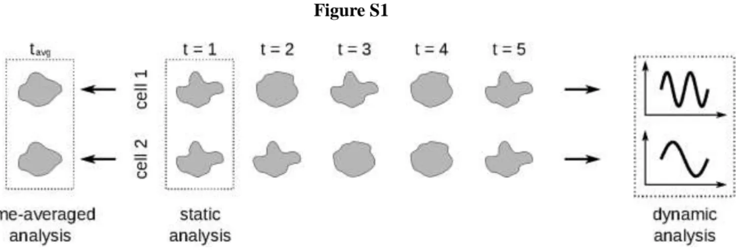
Figure S1: Dynamic shape analysis can reveal patterns that are obscured in static or time-averaged analyses.
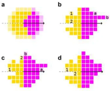
Figure S2: Schematic overview of the parameters of the migration model. (a) Example of a cell with the 𝐹𝑅 (front-rear threshold) parameter > 0; for 𝐹𝑅 = 0, see (b)-(d) and Fig. 1a. (b) Impact of the number of neighbors; removing SU 1 with one neighbor is more likely than removing SU 2 with three neighbors (von Neumann neighborhood); moving the SU into position a with two neighbors is more likely, than into position b with one neighbor. (c) Impact of the position vector; SU 1 is
located closer to the migration axis and therefore has a higher probability of being removed than SU 2; position a is preferred over position b to place the new SU because it is closer to the migration axis. (d) Impact of the distance to the cell's center of mass; SU 1 is located further away from the center of mass and therefore has a higher probability of being removed than SU 2.
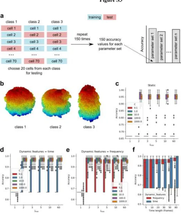
Figure S3: Adjusting classification parameters for synthetic cells. (a) We compute the classifier accuracy for each set of parameters using three-class classification with stratified shuffle split cross-validation. (b) Representative cells from the three analyzed classes. (c) Accuracy of the static classifier for different values of the 𝑙𝑚𝑎𝑥 and 𝐶 parameters. (d) Accuracy of the dynamic time classifier for different values of 𝑙𝑚𝑎𝑥 and 𝐶. (e) Accuracy of the dynamic frequency classifier for different values of 𝑙𝑚𝑎𝑥 and 𝐶. (f) Accuracy of both dynamic classifiers for all values of 𝐶 and
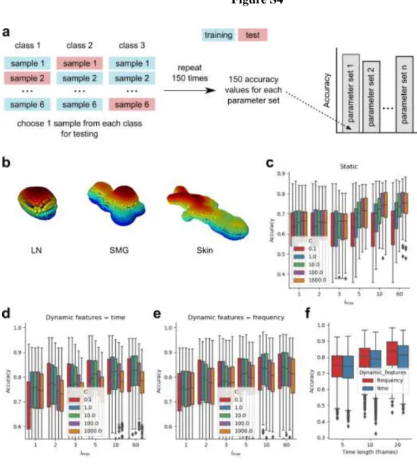
Figure S4: Adjusting classification parameters for T cells. (a) We compute the classifier accuracy for each set of parameters using three-class classification with stratified group shuffle split cross-validation. (b) Representative cells from the three analyzed classes. (c) Accuracy of the static classifier for different values of the 𝑙𝑚𝑎𝑥 and 𝐶 parameters. (d) Accuracy of the dynamic time classifier for different values of 𝑙𝑚𝑎𝑥 and 𝐶. (e) Accuracy of the dynamic frequency classifier for different values of 𝑙𝑚𝑎𝑥 and 𝐶. (f) Accuracy of both dynamic classifiers for all values of 𝐶 and
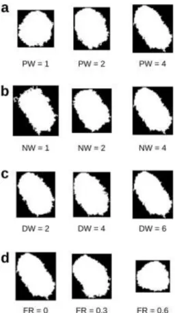
Figure S5: Maximum projections of representative cells generated with three different values of the position weight (PW) (a), neighbor weight (NW) (b), distance weight (DW) (c), and front-rear (FR) (d) parameters. Unless indicated, the default parameter values were used: FR = 0, NW = 4, PW = 4, DW = 6
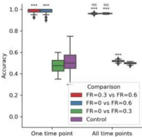
Figure S6: Static classifier accuracy for different pairs of classes relative to control for different values of the FR parameter. Classification was done using either only one (the first) time point of each cell track or all time points. For the parameters other than FR, default values were used: NW = 4, PW = 4, DW = 6. Significant difference from control: *** p<0.001; significant difference from the one-time-point classifier: $$$ p<0.001; two-sided Mann-Whitney test.
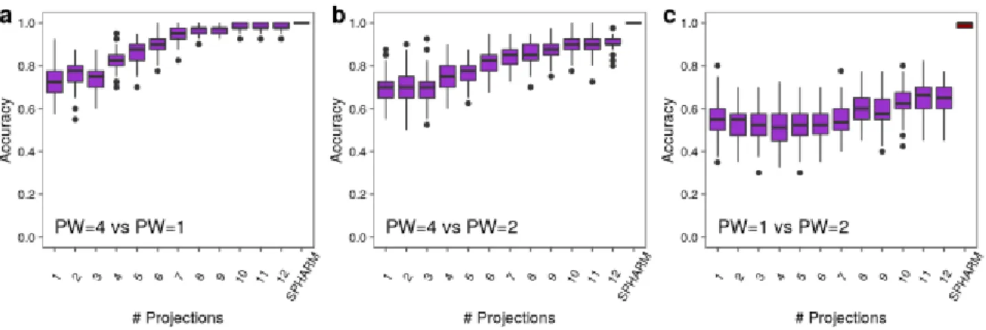
Figure S7: Static SPHARM-based classifier accuracy for synthetic cells of different pairs of classes of the PW parameter in comparison to the DFT-based with projection numbers between 1 and 12. The classes (a) PW=4 versus PW=1, (b) PW=4 versus PW=2, and (c) PW=1 versus PW=2 are compared. For the parameters other than PW, default values were used: NW = 4, FR = 0.0, DW = 6.
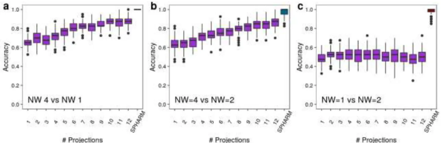
Figure S8: Static SPHARM-based classifier accuracy for synthetic cells of different pairs of classes of the NW parameter in comparison to the DFT-based with projection numbers between 1 and 12. The classes (a) NW=4 versus NW=1, (b) NW=4 versus NW=2, and (c) NW=1 versus NW=2 are compared. For the parameters other than NW, default values were used: PW = 4, FR = 0.0, DW = 6.
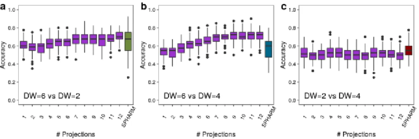
Figure S9: Static SPHARM-based classifier accuracy for synthetic cells of different pairs of classes of the DW parameter in comparison to the DFT-based with projection numbers between 1 and 12s. The classes (a) DW=6 versus DW=2, (b) DW=6 versus DW=4, and (c) DW=2 versus DW=4 are compared. For the parameters other than DW, default values were used: PW = 4, FR = 0.0, NW = 4.
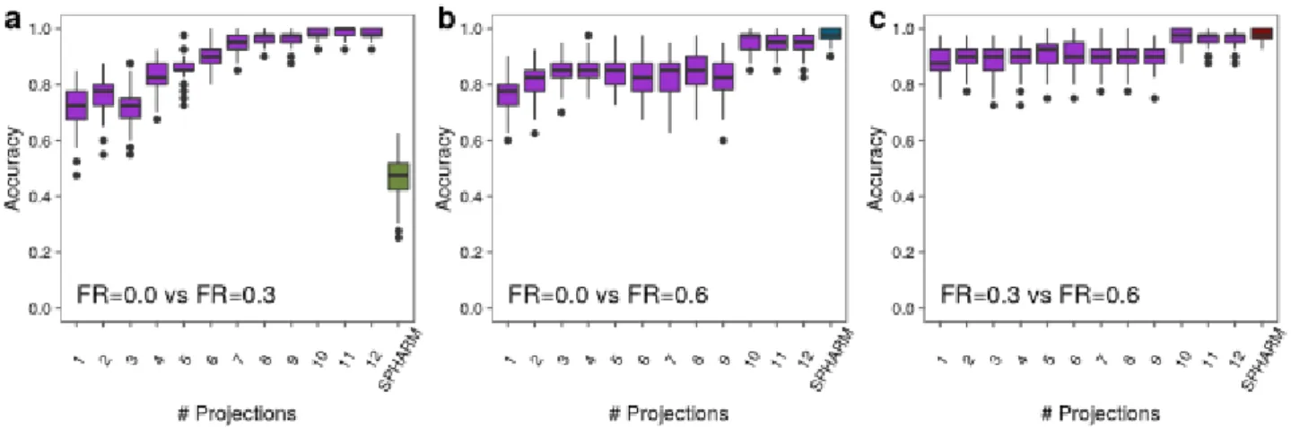
Figure S10: Static SPHARM-based classifier accuracy for synthetic cells of different pairs of classes of the FR parameter in comparison to the DFT-based with projection numbers between 1 and 12. The classes (a) FR=0.0 versus FR=0.3, (b) FR=0.0 versus FR=0.6, and (c) FR=0.3 versus FR=0.6 are compared. For the parameters other than FR, default values were used: PW = 4, DW = 6, NW = 4.
Anna Medyukhina1, ‡,†, Marco Blickensdorf1,†, Zoltán Cseresnyés1, Nora Ruef3, Jens V. Stein3, Marc Thilo Figge1,2,4,*
1Applied Systems Biology, Leibniz Institute for Natural Product Research and Infection Biology – Hans Knöll Institute (HKI), Jena, Germany. 2Institute of Microbiology, Faculty of Biological Sciences, Friedrich Schiller University Jena, Jena, Germany.
3Department of Oncology, Microbiology and Immunology, University of Fribourg, Fribourg, Switzerland. 4Center for Sepsis Control and Care (CSCC), Jena University Hospital, Jena, Germany.
‡ This author’s current affiliation is Center for Bioimage Informatics, St. Jude Children’s Research Hospital, Memphis, TN
† These authors contributed equally to this work.
* Correspondence should be addressed to M.T.F.: [email protected]
Experimental data
Mice
OT-I TCR1 were backcrossed to Tg(UBC-GFP)30Scha “Ubi-GFP”2 or hCD2-dsRed3 mice. 6-10 week-old sex-matched C57BL/6 mice (Janvier, France) were used as recipient mice. All mice were maintained at the animal facility of the Department of Clinical Research/University of Bern or at the University of Fribourg. All animal work has been approved by the Cantonal Committee for Animal Experimentation and conducted according to federal guidelines.
T cell transfer and viral infections
CD8+ T cells were negatively isolated from spleen and peripheral lymph nodes of GFP+ or dsRed+ OT-I, using the EasySep Mouse CD8+ T Cell Isolation Kit (Stem Cell Technologies). OT-I T cells (5 x 10⁴)were i.v. transferred into recipient mice 24 h before i.p. infection with 105 pfu LCMV-OVA4. For skin imaging, 15 µl 0.3% DNFB (in acetone/oil 4:1) was applied to the right flank on day 3 p.i. and 500 ng SIINFEKL peptide was applied on days 4 and 5 p.i.. Two-photon microscopy (2PM) imaging was performed ≥ 30 days p.i..
2PM image acquisition and analysis
2PM intravital imaging of the popliteal lymph node, SMG, and skin was performed as described
5,6. In brief, mice were anesthetized with ketamine/xylazine/acepromazine, and for lymph node
(LN) imaging the right popliteal lymph node was surgically exposed. Before recording, Alexa 633-conjugated MECA-79 (10 µg/mouse) was injected i.v. to label HEV. For submandibular salivary gland (SMG) imaging, the right SMG lobe was surgically exposed. For skin imaging, a section of the right flank skin was elevated onto a metal holder by making two parallel incisions.
2PM imaging was carried out with a TrimScope 2PM system (LaVision Biotec) using a 25X Nikon (NA 1.0) objective. ImSpector software was used to control the 2PM system and acquire
z-step size of 2-4 µm were acquired in 0-140 µm depth. The time interval was 20 s for LN and SMG and 60 s for the skin and the imaging time was 20-60 minutes. Emitted light and second harmonic signals were detected through 447/55-nm, 525/50-nm, 593/40-nm and 655/40-nm bandpass filters with non-descanned photomultipliers.
Image preprocessing
Two-photon intravital images were provided as OME-TIFF images, which were converted to single time point and single Z layer TIFF images using a custom-written ImageJ macro. These images were loaded into HuygensPro 19.04 (SVI, Hilversum, Holland) in order to be deconvolved. The deconvolution process was carried out by using the theoretical point spread function (PSF), as provided by HuygensPro’s Classic Maximum Likelihood Estimation method, based on the
Richardson-Lucy algorithm. The deconvolved images were saved as multilayer TIFF files, one image stack per time point.
T-cell segmentation and tracking
The deconvolved time-series images were loaded into Imaris 9.3.1 (Bitplane, Zürich,
Switzerland) for further processing. In the first step, the image stacks were thresholded with the Otsu algorithm in order to identify the voxels that belonged to the foreground, representing the fluorescently labeled T-cells. Typically the threshold values allowed the fluorescence range of 1000 to 15000 to be considered as part of the reconstructed cell surface. The T-cells were then segmented as 3D surfaces using the Surfaces object-creation wizard of Imaris. The surface rendering was adjusted to the complex cell shape of the active T-cells by setting the smoothing scale to 0.2 micrometers and the local threshold search radius to 1.0 micrometer, in order to make the Surfaces objects fit the volume image of the T-cells precisely. Objects below the volume of 1500 voxels were eliminated, in order to avoid detecting debris.
In the next step of the analysis, the reconstructed surfaces that represented individual T-cells were tracked. For this, the Autoregressive Motion tracking method of Imaris was applied, with a maximum allowed gap size of one time step, and a minimum track length corresponding to 50% of the total duration of the experiment. Each time series of the reconstructed and tracked images were individually observed in the next step of the analysis, in order to identify potential tracking errors caused by multiple T-cells forming a temporary cluster that would have been identified as one large cell. Such artificial clusters were manually removed from further analysis. These corrections were
parsed by a customized Python script to extract the surface coordinates of individual cells, which were then combined into time-series with the help of the track files.
Adjusting the classification parameters
Before applying the classifier to distinguish between types of migrating cells, several parameters of the classification and the feature extraction workflow had to be adjusted. First, we needed to choose the number of SPHARM degrees lmax used in the analysis. Second, for the dynamic analysis, we needed to select the number of analyzed time points T. Finally, the penalty parameter C of the SVM classifier had to be adjusted to obtain the optimal classification results. Whereas the first two parameters (lmax and T) determine the number of features used for classifications, parameter C
defines how well classification errors are tolerated by SVM while fitting the training data. With small values of C, more errors are tolerated, whereas, with large C values, SVM tries to classify the training dataset with as high accuracy as possible.
To choose the optimal values of these parameters for synthetic data, we generated a synthetic dataset of 210 cells from three visually distinct classes (Fig. S2b). For each parameter combination, we performed 100 rounds of cross-validation with stratified shuffle split, where 5/7 of the data (50 cells from each class) were randomly chosen as the training set, and 2/7 (20 cells from each class) served as the test set (Fig. S2a). The accuracy of the classifier was evaluated for all parameter combinations and all three feature vectors (Fig. S2c-f), and the parameters that provided the highest accuracy for all three feature vectors were chosen for further analysis (lmax=2, C=100, T=80).
The parameter adjustment for T cells was performed similarly, but the stratified shuffle split was replaced by stratified group shuffle split, where one time-series from each class was used for testing and the rest (five time-series) were used for training (Fig. S3a). Similarly to synthetic cells, cross-validation was carried out for 100 rounds for each parameter combination, and the accuracy of the classifier was quantified for both static and dynamic features (Fig. S3c-f). Due to the limited duration of the T cell tracks, we had to use fewer time points than in synthetic data (T=10). Also, a higher value of lmax (lmax=10) had to be used, likely in order to increase the size of the feature vector and thus to compensate for the small value of T. For the C parameter, different values were optimal for the static and dynamic analysis, and therefore C=100 was chosen for the static classifier and C=10 was chosen for both dynamic classifiers.
2. Schaefer, B. C., Schaefer, M. L., Kappler, J. W., Marrack, P. & Kedl, R. M. Observation of antigen-dependent CD8+ T-cell/dendritic cell interactions in vivo. Cell. Immunol. (2001). doi:10.1006/cimm.2001.1895
3. Kirby, A. C., Coles, M. C. & Kaye, P. M. Alveolar Macrophages Transport Pathogens to Lung Draining Lymph Nodes. J. Immunol. (2009). doi:10.4049/jimmunol.0901089 4. Kallert, S. M. et al. Replicating viral vector platform exploits alarmin signals for potent
CD8+ T cell-mediated tumour immunotherapy. Nat. Commun. (2017). doi:10.1038/ncomms15327
5. Ficht, X., Thelen, F., Stolp, B. & Stein, J. V. Preparation of murine submandibular salivary gland for upright intravital microscopy. J. Vis. Exp. (2018). doi:10.3791/57283
6. Moalli, F. et al. The Rho regulator Myosin IXb enables nonlymphoid tissue seeding of protective CD8+ T cells. J. Exp. Med. (2018). doi:10.1084/jem.20170896
7. Vladymyrov, M., Abe, J., Moalli, F., Stein, J. V. & Ariga, A. Real-time tissue offset correction system for intravital multiphoton microscopy. J. Immunol. Methods (2016). doi:10.1016/j.jim.2016.08.004
non-transparent Surfaces view by the time series reaches the halfway point. The video then fades the Surfaces objects down to 57% transparency by the end of the image series. The video then resets to the original volume view as seen at zero time point. The view of the video is set at 45 degrees perspective. The scale bar indicates the calibrated size of the scene. Video S3: CD8+ T cells migrating in a submandibular salivary gland. For details of video creation see the caption of Video S2.
Video S4: CD8+ T cells migrating in skin. For details of video creation see the caption of Video S2.