A Formally-Proved Algorithm to Compute the Correct Average of Decimal Floating-Point Numbers
Texte intégral
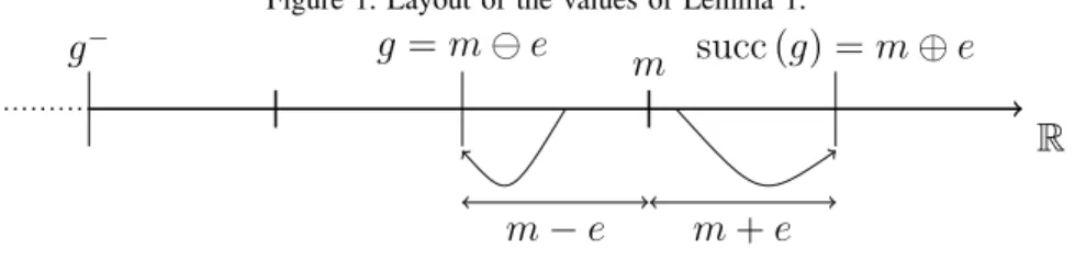
Figure
Documents relatifs
• with the directed roundings, for implementing interval arithmetic in a trustable yet accurate way: in round-to-nearest mode, correct rounding provides an accuracy improvement
This chapter is an introductory chapter: it recalls the definitions related to floating-point arithmetic, and presents some of the features of the IEEE-754-2008 Standard for
The IEEE standard does not require correct rounding of other functions than the square root and the four arithmetic operations.. This is mainly due
As is known from work of Alladi [All87] and Hildebrand [Hil87], the number ω(n) of prime factors of n ∈ S(x, y) typically tends to grow with n, in such a way that we may expect the
Physically, this means that at energies of this order pions (which are the lightest hadrons) can be produced in collisions of protons in cosmic rays with CMB photons, which prevents
There exists a positive real constant C such that for any positive integer n and any deterministic and complete transition structure T of size n over a k-letter alphabet, for
Pour la commodité du lecteur nous rappelons ici les principaux résultats dont nous aurons besoin.. Ces deux étapes onL peu de choses en commun. Dans certains cas c'est difficile
Pressure needed to reduce to in order to fully open valve if partially closed Actuator position error.. Change in pressure needed to fix position error Pressure
