Currency Choice and Exchange Rate Pass-Through
Texte intégral
Figure
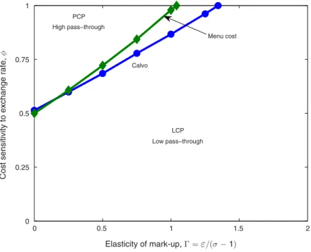
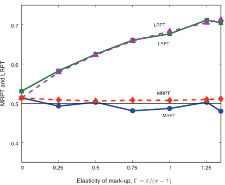
![Figure 4 carries out a similar exercise, but now holds Γ = 0.75 ( i.e., ε = 3 ) constant and varies ϕ on [ 0.5, 1 ]](https://thumb-eu.123doks.com/thumbv2/123doknet/14530091.533390/23.756.149.608.101.472/figure-carries-out-similar-exercise-holds-constant-varies.webp)
Documents relatifs
We examine responses of domestic prices to a positive one unit exchange rate shock by estimating a Threshold Vector Autoregression (TVAR) model.. The exchange rate
Source: IMF’s Classification of Exchange Rate Arrangements and Monetary Frameworks RR de facto exchange rate regime: Binary variable taking the value 1 if in a given year a country
This analysis leads to a rethinking of the monetary policy regimes (targets), adopting a hybrid targeting (quantitative monetary objective and targeting the exchange
index, and (v) fitting the refractive index to obtain the material parameters. This process has shown promising results, but has several drawbacks as previously described. The
cycle. Petrášek, Probing plant membranes with FM dyes: Tracking, dragging or blocking? Plant J. Weaver, Extracellular vesicles: Unique intercellular delivery vehicles. Trends
In sum, because IT is associated to a greater PT when the oil price falls, there is an almost symmetric impact of oil price changes on inflation in these countries. For instance,
Thus, we expect the extent of pass-through would be different with respect to the business cycle, that is, the transmission of exchange rate changes would be higher when economy
It is known that impulse responses trace the effects of a shock to one endogenous variable on to the other variables in the VECM system, allowing us to estimates of the effect
![[PDF] Cours sur le langage C++ apprendre les principaux savoir-faire | Cours informatique](data:image/gif;base64,R0lGODlhAQABAIAAAP///wAAACH5BAEAAAAALAAAAAABAAEAAAICRAEAOw==)