Contraction/expansion flow of dilute elastic solutions in microchannels

(1)

Contraction/Expansion Flow of Dilute Elastic Solutions in Microchannels

by

Timothy Peter Scott

B.S. Mechanical Engineering Tufts University, 2002

SUBMITTED TO THE DEPARTMENT OF MECHANICAL ENGINEERING IN PARTIAL FULFILLMENTOF THE REQUIREMENTS FOR THE DEGREE OF

MASTER OF SCIENCE IN MECHANICAL ENGINEERING AT THE

MASSACHUSETTS INSTITUTE OF TECHNOLOGY JUNE 2004

The author hereby grants to MIT permission to reproduce and to distribute publicly paper and electronic

copies of this thesis in whole or in part.

Signature of Author: Department of Certified by:

U)

Professor of Mechanical Engineering ,May 7, 2004 ,7/Areth H. McKinley Mchanical Engineering Thesis Supervisor Accepted by: ____ Ain A. Sonin MASSACHUSETTS INS__N_ _ Professor of Mechanical Engineering

OF TECHNOLOGY

(2)

(3)

Contraction/Expansion Flow of Dilute Elastic

Solutions in Microchannels

by

Timothy Peter Scott

Submitted to the Department of Mechanical Engineering on May 7, 2004 in Partial Fulfillment

of the Requirements for the Degree of Master of Science in Mechanical Engineering

ABSTRACT

An experimental study is conducted on the nature of extensional flows of mobile dilute polymer solutions in microchannel. By observing such fluids on the microscale it is possible to generate large strain rates (~ 50,000 s-) that are greater than values which have been observed in macroscale contraction flows. Subsequently, large Deborah numbers (equivalent to those observed on the macro scale in high viscosity solutions) are generated for low viscosity solutions without the interplay of significant inertial effects. High quality microfluidic channels are fabricated using soft lithography techniques. Rheological behavior in these channels is dominated by an abrupt planar contraction, which generates extensional flow in the working fluids. Dilute viscoelastic aqueous solutions of polyethylene oxide are passed through 16:1 planar micro-contractions. Fluids exhibit substantial elastic behavior marked by elastic instabilities followed by subsequent lip vortices and eventually stable vortex growth. The onset of flow instabilities (De =50) and the nature of vortex growth are similar for PEO solutions at various concentrations. Differential pressure measurements indicate that substantial extensional thickening occurs at the onset of flow instabilities and indicate that planar extensional viscosities grow rapidly with increasing strain rates. Also apparent Trouton ratios are calculated indicating that extensional viscosities are two orders of magnitude larger than shear viscosities at high Deborah numbers.

Thesis Supervisor: Gareth H. McKinley Title: Professor of Mechanical Engineering

(4)

List of Figures

Figure 1-1. (a) Image of the mixer used by Groisman and Steinberg to enhance mixing. (b) Mixing of Newtonian solvent after passing through the mixer at low Reynolds Number (Re = 0.16). (c) Image of the polymeric solution showing extensive mixing at the same flow rate corresponding to a Deborah number of 6.7 (Groisman and

S teinb erg , 2 0 0 1)... . 16

Figure 1-2. An image of the nonlinear resistor developed by Groisman et al. at varying applied pressures. Beyond a critical pressure (~30 Pa) large changes in pressure only correspond to moderate changes in flow rate (Groisman et al., 2003). ... 17

Figure 1-3. Flow rate dependence on applied pressure drop for the nonlinear resistor proposed by Groisman et al. (Groisman et al., 2003). ... 18

Figure 1-4. Microfluidic flip-flop used by Groisman et al. for controlling flow directions ... ... 18

Figure 1-5. Streakline patterns for microfluidic rectifier at different applied pressures. Flow travels forward for pictures (a) -(d) and backward for pictures (e) -(h). The images show the irreversibility of the polymer solutions in microchannels caused by elastic instabilities (Groisman and Quake, 2004). ... 20

Figure 1-6. Flow rate -pressure dependence of the microfluidic rectifier. Circles indicate forward flow (left to right), while squares are backward flow (Groisman and Quake, 2 0 0 4 ). ... 2 0 Figure 1-7. Creeping contraction flow of a Newtonian fluid: comparison of experimental results and computational simulations (Boger et al., 1986)... 22

Figure 1-8. Inkjet printing cartridge: a micro-entry flow of a non-Newtonian fluid... 23

Figure 1-9. Images of a micro-contraction used for flow focusing of emulsions. The contraction is used to generate emulsion droplets (Anna et al., 2003) ... 23

Figure 1-10. Extensional viscosity of various PEO solutions using a opposed jet rh eo m eter ... 2 5 Figure 1-11. MR fluid used as a valve to stop fluid flow. Fluid initially flows through channel (left). Upon applying a magnetic field, flow is stopped (right) (image courtesy of R am in H aghgooie). ... 28

Figure 1-12. Shear-free planar flow ... 30

Figure 1-13. Dimensions of microchannels used in the present study ... 30

Figure 2-1. Axisymmetric contraction, as used in previous macroscale studies ... 33

Figure 2-2. Vortex growth for a Boger fluid in an axisymmetric contraction (Rothstein and M cK inley, 1998). ... 35

Figure 2-3. Three different vortex regimes observed in axisymmetric contractions... 36

Figure 2-4. Different vortex growth regimes determined based upon contraction ratio and Deborah number (M cKinley et al., 1991)... 37

Figure 2-5. Plot of the Deborah number versus the Reynolds number and associated vortex regimes for entry flow experiments... 38

Figure 2-6. Comparison of the dimensionless flow parameters of previous planar contraction studies performed on the macroscale... 42

Figure 2-7. Comparison of the dimensionless flow parameters for experiments, accounting for rate-dependant rheological properties... 43 Figure 2-8. Planar contraction results for a Boger Fluid in an 80:1 contraction (left)

(7)

contraction (center) (Evans and Walters, 1989): Re = 7.5, De = 2.7, and a 0.1 % PAA solution in a 10:1 contraction (right) (Chiba et al., 1990): Re = 89, De = 4.6. 44 Figure 2-9. Flow rate versus applied pressure for the contraction flows of Boger fluids

(N igen and W alters, 2002)... 45 Figure 2-10. Sources of pressure loss along the microchannels ... 49 Figure 2-11. Sample Bagley plot: pressure drop is extrapolated to zero contraction length

... 4 9 Figure 2-12. Comparison of several techniques for predicted extensional viscosity with

data obtained using Phan-Thien-Tanner constitutive model at a strain of 0.5. Results show good agreement with simulations especially at high shear rates (Raj agopalan, 2 0 0 0 ). ... 5 2 Figure 3-1. Fabrication process used in the present study ... 56 Figure 3-2. SU-8 Mold without contrast enhancer (left) compared with mold using

contrast enhancer (right) ... 58 Figure 3-3. Comparison of the SU-8 mold from a transparency mask (left) and a chrome

mask (right). Both were generated using the contrast enhancer. ... 59 Figure 3-4. Im age of cracks in SU-8 2050 mold ... 60 Figure 3-5. SEM image of PDMS channels and the cracks generated in the SU-8 baking

p ro c e sse s ... 6 1 Figure 3-6. Entry of 160:10 tm channel... 62 Figure 3-7. Setup of pressure measurement system... 65 Figure 3-8. Plot of the calibration curves used for the three different pressure sensors... 66 Figure 3-9. Pressure increase with time for increasing flow rates (0 ml/hr -6 ml/hr). Flow

rates are increased 1 ml/hr every 5 minutes. Data is taken using a Newtonian 55% glycerol and water mixture (ro = 8.59 mPa-s) in a 400:25 ytm contraction. Time lag is on the on the order of 5 minutes at the lowest flow rates, but decreases as flow rate in creases... 6 7 Figure 3-10. Figure shows lag times for the 0.1% polyethylene oxide solution at

increasing flow rates. This figure shows the time range over which pressure

m easurem ents are averaged. ... 67 Figure 3-11. Sample PDMS channel for length measurement: nominally a 400:25 ym

contraction, measured values are within 5% of the designed dimensions... 71 Figure 3-12. Cross section of 160 ,Im channel, used for measuring channel depth ... 72 Figure 4-1. Molecular weight plotted against concentration. This figure shows the

different solvent regimes based on various polymer concentrations and molecular weights. Adopted from (Dontula et al., 1998). ... 73 Figure 4-2. Schematic of double gap Couette cell for AR2000... 79 Figure 4-3. Rheological data for fluids employed in this study... 80 Figure 4-4. Effects of PEO concentration on power law index and zero-shear-rate

viscosity. Values for zero-shear-rate viscosity are compared with dilute polymer solution prediction . ... . . 83 Figure 4-5. Schematic of CABER setup (picture adopted from (Verani and McKinley,

2 0 0 4 )) ... 8 6 Figure 4-6. High-speed video of capillary thinning on CABER for 0.1% PEO, 0.3% PEG,

and 0.1% PEO + 55% Glycerol. Images are taken at six equal intervals from when the plates are fully separated until filament break-up ... 90

(8)

Figure 4-7. CABER results at the lowest aspect ratio (A = 1.41). 0.1% PEO in 55% glycerol and water data shows oscillations at the Rayleigh frequency... 91 Figure 4-8. CABER results from medium aspect ratio (A = 1.61)... 92 Figure 4-9. Relaxation time average over 5 trials for each aspect ratio. For each fluid, the

dependence on the aspect ratio is weak and appears random. For the less viscous fluids at low aspect ratios the data was either precise (within 10%) or completely inaccurate, and therefore ignored. As a result, error bars for these fluids are small. 92 Figure 4-10. Images of droplet formations in 0.1% PEO which cause errant data at high

aspect ratios (A = 2.02) (Image courtesy of Lucy Rodd) ... 93 Figure 4-11. Images of the damped oscillations of the lower droplet which can interfere

with CABER measurements. Images are taken for the 0.1% PEO in 55% glycerol and water solution at an aspect ratio of A = 1.41 ... 93 Figure 4-12. Comparison of the thinning data of a polymer solution (0.1% PEO + 55%

Glycerol and Water) and a Newtonian fluid (55% Glycerol and Water). Data is taken at aspect ratios of A = 1.41 and A = 1.22, respectively. ... 94 Figure 5-1. Streak images for DI water in 400:25

stm

contraction showing the growth of

exit vortices (a) Re = 5.5 (b) Re = 8.3 (c) Re = 14 (d) Re = 22 (e) Re = 33 (f) Re =

4 4 ... 9 9 Figure 5-2. Streak images for the 0.1% PEO solution (El = 11.7). (a) De = 27.6, Re =

2.35 (b) De = 41.3, Re = 3.52 (c) De = 55.1, Re = 4.69 (d) De = 96.4, Re = 8.21 (e)

De = 110, Re = 9.39 (f) De = 124, Re = 10.6 (g) De = 165, Re= 14.1 (h) De = 220, R e = 1 8 .8 ... 10 1 Figure 5-3. Technique used for measuring vortex lengths: upstream width is measured as

W,= 400

stm

and rotated to measure vortex length, L ... 103 Figure 5-4. Dimensionless vortex length plotted against Deborah number for the 0.1%

P E O so lu tio n ... 10 3 Figure 5-5. Streak images of the 0.3% PEO solution (El = 126) (a) De = 41.2, Re = 0.33

(b) De = 61.7, Re = 0.49 (c) De 82.3, Re = 0.65 (d) De = 103, Re = 0.82 (e) De = 123, Re = 0.98 (f) De = 144, Re =1.1 (g) De = 165, Re = 1.31 (h) De = 247, Re = 2.0 (i) De = 330, Re = 2.62 (h) De = 494, Re = 3.9... 106 Figure 5-6. Transient images of the secondary vortex for the 0.3% PEO solution in the

16:1 contraction (De = 494). Images are taken every 200 ms. ... 107 Figure 5-7. Dimensionless vortex lengths for both the 0.1% PEO and 0.3% PEO

solutions. The vortex lengths of the two fluids appear to collapse onto a single line of slope 0.0026 (R 2 = 0.9 1)... 108

Figure 5-8. Dimensionless vortex lengths plotted against Reynolds number: no

correlation is seen ... 10 8 Figure 5-9. Streak images of the 0.3% PEO solution in a 4:1 contraction (200:50

stm)

(El

= 31.2). (a) De = 40, Re = 1.28 (b) De = 61, Re = 1.95 (c) De = 81, Re = 2.60 (d) De = 12 1, R e = 3 .8 8 ... 1 10 Figure 5-10. Pressure losses accrued between pressure taps ... 112 Figure 5-11. Pressure loss ratio for power-law fluid estimate compared with Newtonian

fluid as a function of the power-law index (n) for channel of the same dimensions of the contraction (W, = 25 pm , h = 50 pm ). ... 115 Figure 5-12. Comparison of the predicted pressure loss based on Newtonian and

(9)

and 0.3% PEO solutions. Pressure loss data for the circular and infinite planar cross section are indistinguishable... 116 Figure 5-13. Measured pressure versus flow rate data for 400:25 Am contraction (L, = 50

pt m ) for all flu id s ... 1 17 Figure 5-14. Measured pressure versus flow rate data for 400:25 Itm contraction (Le =

100 tim ) for all flu id s ... 118 Figure 5-15. Measured pressure versus flow rate data for 400:25 Jim contraction (Lc =

4 00 jtm ) for all flu ids ... 118 Figure 5-16. Range of pressure drops for maximum shape factor (C = 96) and minimum

(C = 56.9) compared with the actual pressure loss data for DI water in each

contraction (a) Lc = 50 tim (b) Lc = 100 itm (c) L, = 400 tim ... 121 Figure 5-17. Hole pressure effect: tension in streamlines cause recessed pressure sensors

(PI h) to read less than that of a flush mounted transducer (P,,) (picture source: (M aco sk o , 19 94 ))... 12 2 Figure 5-18. Pressure measurements are conducted on three different trials using the L=

400 tim contraction for the 0.1% PEO solution to show repeatability for the same fluid and geometry. Measured pressures are compared with Newtonian and power-law calcu latio n s... 12 4 Figure 5-19. (a) Pressure loss data for a W = 57 tm straight channel. Measured data is

compared with Newtonian and power-law predictions for pressure drop. (b) Darcy friction factor (J) is plotted against Reynolds number ... 125 Figure 5-20. Normalized pressure data (with respect to the Newtonian prediction:

equation (5.1)) for the DI water in each contraction... 126 Figure 5-21. Normalized pressure data for the 0.1% PEO solution in each contraction.

Pressure is normalized against the Newtonian prediction (equation (5.1)) (left) and the power-law prediction (from equation (5.10)) (right) ... 127 Figure 5-22. Normalized pressure data for the 0.3% PEO solution in each contraction.

Pressure is normalized against the Newtonian prediction (equation (5.1)) (left) and the power-law prediction (from equation (5.10)) (right) ... 128 Figure 5-23. Pressure loss normalized by the tangential pressure drop from the linearly

in creasin g region ... 12 9 Figure 5-24. Apparent extensional viscosity plotted against strain rate for the 0.05% PEO, 0.1% PEO, and 0.3% PEO solutions as calculated for the 400-micron contraction132 Figure 5-25. Trouton ratio plotted against Deborah number for 0.05% PEO, 0.1% PEO,

and 0.3% PEO solutions as calculated for the L, = 400 tim contraction ... 133 Figure 5-26. Trouton ratio plotted against Deborah number for the 0.1% PEO solution in

each con traction ... 134 Figure 5-27. Trouton ratio plotted against Deborah number for the 0.3% PEO solution in

each con traction ... 134 Figure 5-28. Schematic showing the extension and relaxation of a polymer across the

co n tractio n ... 13 6 Figure 5-29. Dimensionless residence times (Der) plotted against flow rate for the 0.1%

PE O and 0.3% PE O solutions... 136 Figure 6-1. Predicted vortex regimes based on the Reynolds and Deborah number for a

(10)

Figure 6-2. Sample micro PIV for water in 16:1 contraction. Field of view is too small to resolve velocities near the contraction... 141 Figure 6-3. Schematic of the nanopore created by U.S. Genomics to unravel single

(11)

List of Tables

Table 2-1. Review of Cogswell's method and its applications (A/P* -axisymmetric or p lan ar) ... 5 5

Table 3-1. Summary of pressure sensors specifications ... 65

Table 3-2. Measured dimensions compared with specified dimensions... 70

Table 4-1. Polymer architecture for PEO (Mw = 2,000,000 g/mol). (Value for v from (Tirtaatmadja et al., 2004), C, from (McKinley and Armstrong, 2000))... 78

Table 4-2. Rheological data from double gap Couette cell ... 82

Table 4-3. Relaxation times for fluids used in the present study... 95

Table 4-4. Sum m ary of fluid properties... 97

Table 5-1. Sampson pressure drop as a percentage of total Poiseuille pressure drop for various channels and contraction ratios ... 113

(12)

1

Introduction

In recent years advances on the microscale have modified the landscape of many technical fields, including that of fluid mechanicians. The development of microfluidics has renewed interest in many of the classical fluids problems which had been solved in previous years. The microfluidics community is rapidly growing, and the "lab-on-a-chip" phenomenon is becoming applicable to nearly all scientific disciplines. The introduction of rapid prototyping (Effenhauser et al., 1997; Duffy et al., 1998) has now increased the accessibility to microfluidics, making dramatic advances in the field, in both depth and bredth, inevitable.

1.1 Microfluidics

The term microfluidics refers to fluidic devices with smallest feature sizes at lengthscales of one micron or greater. Microfluidic endeavors have focused on various topics ranging from biological systems to fluidic circuitry. And with increasing amounts of research focused on microfluidic technologies, the potential applications of this research are virtually unbounded.

Microfluidic devices have become critical components of various scientific and medical applications. Such small-scale systems are ideal for many chemical and biological

endeavors for which small sample sizes and accurately defined geometries are imperative. Microfluidic systems have been developed to assist in the analysis and

separation of deoxyribonucleic acid (DNA) (Effenhauser et al., 1997; Chou et al., 1999). Also microfluidic devices have been employed in microfluidic networks with

immunoglobins for subsequent assays (Delamarche et al., 1997). These devices have also been employed for cell sorting and cell analysis (Fu et al., 1999). The ultimate goal of microfluidic research is to develop Micro Total Analysis Systems (yTAS), which are capable of performing all sample analyses within one microfluidic chip. However, one of

(13)

the limiting factors on this research has been the inability to effectively generate simple valves and pumps to control transportation of samples between analysis chambers.

There are several means of fabricating microfluidic systems, each of which have their own benefits and applications. Soft lithography has become the most utilized means of microfluidic generation in recent years based on its simplicity, cost, efficiency, optical transparency, and compatibility (Quake and Scherer, 2000; Stone and Kim, 2001). Soft

lithography uses photolithography to develop a mold off which multiple elastic polymer channels may be reproduced. This polymer can be bonded to glass surfaces and allows for simple fabrication of accurate microchannels. Other techniques for developing microchannels include etching into surfaces such as silicon or glass. These techniques,

originally the backbone of microfluidics, are being used less due to the cost and time of fabrication (Quake and Scherer, 2000; Stone and Kim, 2001). Recently techniques have been developed which use chemical modification of surface properties to define

microfluidic boundaries (Zhao et al., 2001). These techniques define hydrophobic boundaries to confine flow to hydrophilic regions, but these channels are only able to withstand small pressures.

In microfluidic channels there are several means of developing flow within the network. The simplest method is by creating a pressure gradient across the channel, either by applying pressure at the input or a vacuum at the outlet. These techniques are capable of generating large flow velocities, but require fluids to adhere to the physics of developed pipe flow (parabolic velocity field). Another common technique for driving flow fields in microfluidics is electrophoresis, which involves the use of electrically charged particles which are set into motion by an imposed electric field. This technique allows for a uniform flow field, but it is limited in achievable velocities. Other techniques involve the usage of concentration gradients to stimulate osmotic movements within microchannels. Lastly, boundary conditions, such as surface evaporation, capillary forces, or surface permeability can be used to induce fluid motion. However, the only technique that can generate large flow velocities (> 1 mm/s) in a liquid filled medium is the application of an external pressure gradient.

(14)

1.2 Complex Fluids in Microchannels

Non-Newtonian fluids are fluids that appear homogenous on the macroscale but actually have a complex internal microstructure. Because of this internal structure, the properties of these complex fluids can change based on the lengthscales and timescales of

associated flows (Bird et al., 1987). Many non-Newtonian fluids are marked by

substantial elastic and viscous properties which, unlike and Newtonian fluids, can lead to counterintuitive flow and stress response. The nature of this elasticity is encapsulated in a relaxation time, which is the timescale over which the fluid is able to return to a

stress-free condition: larger relaxation times are indicative of more elastic fluids.

Microfluidics as a field has its roots in observing non-Newtonian fluids. Some of the earliest microfluidic devices were designed to test the flow of biological fluids in channels constructed of silicon, designed on the same lengthscale as human capillaries (Karlsson et al., 1991; Wilding et al., 1994). These fluids contain large microstructures (such as proteins, DNA, or blood cells) which can generate highly non-Newtonian behavior in the fluids. Works were primarily focused on the biological aspects of the blood cell behavior, however bulk fluid viscosity was considered. Yet in these studies, the elastic properties of the fluids were always neglected or not understood. There has been little effort to focus on the rheological aspects of complex fluid flow on the microscale.

Groisman and Steinberg examined the use of polymeric liquid in for the purpose of enhanced mixing (2001) in small geometries (3 mm). While these were not

microchannels, the small lengthscales involved restrict fluids to low Reynolds numbers and laminar flow, which is typical of microfluidics. In laminar flow of Newtonian fluids, the primary means of mixing fluids is through diffusion. Because diffusion is small over the timescales frequently considered (~ 100 ms), enhancing fluid mixing is frequently a challenge for many microfluidic devices. Groisman and Steinberg investigated the use of polymeric liquids to enhance mixing at low Reynolds numbers.

(15)

The experiments of Groisman and Steinberg involved dissolving a small amount (800 parts per million) of high molecular weight (M,) polymer (polyacrylamide: M,

18,000,000 g/mol) in a Newtonian solvent. Then they compared the mixing of this solution with the mixing of just the Newtonian solvent. The basis for using this polymer was to reach the onset of elastic instabilities in the fluid and, therefore, enhance mixing. This technique is similar to macroscale mixing in which the critical Reynolds numbers are exceeded to induce turbulent mixing. However, for elastic instabilities the critical parameter for the onset of instabilities is the Deborah number (or Weissenberg number):

De = Af (1.1)

where Xis the fluid's relaxation time and ' is the characteristic shear rate. When the

Deborah number becomes large the fluid elements are being sheared faster than they can relax, thus instabilities occur (Bird et al., 1987) and mixing is enhanced (Groisman and Steinberg, 2000).

These experiments made use of the large shear rates generated in small channels to induce elastic instabilities in their viscoelastic solutions. They dyed the two fluid inlets different colors to distinguish between the two flows (see figure 1-1). For the Newtonian solvent, little mixing was observed (only that of diffusion), but for the polymer solution, significant mixing occurs. Clearly the elastic instabilities are the driving force behind allowing the two solutions to mix. They also examined concentration dependence of their mixing device and determined that mixing was observed at concentrations as low as 7 ppm (parts per million) and showed that mixing could be enhanced in even high viscosity solutions with Reynolds numbers as small as 0.0 16. However, the paper fails to

adequately analyze several of the rheological aspects (only the bulk viscosity and characteristic relaxation time are given), which dictate the behavior of the fluids in such geometries.

(16)

Figure 1-1. (a) Image of the mixer used by Groisman and Steinberg to enhance mixing. (b) Mixing of Newtonian solvent after passing through the mixer at low Reynolds Number (Re 0.16). (c) Image of the polymeric solution showing extensive mixing at the same flow rate corresponding to a Deborah number of 6.7 (Groisman and Steinberg, 2001).

First, the analysis focuses on observing the mixing in smooth rounded channels, however, there is little reason that such a geometry would enhance fluid mixing. In fact, sharper and smaller geometries would enhance mixing by initializing elastic instabilities more quickly. Stress singularities develop at such corners and have been the source of elastic instabilities in many macroscale experiments (Bird et al., 1987), while rounded corners tend to suppress elastic behavior (Evans and Walters, 1986; Evans and Walters, 1989). Fluid instabilities are observed at Deborah numbers of 3.2, which is greater than unity, but little explanation was offered for the delayed onset of elastic behavior. Also, in considering concentration effects, they failed to quantify relaxation times as the

concentration decreased. Thus they did not determine if the critical Deborah number for mixing was consistent with the Deborah number for the initial polymer solutions

observed.

In the laboratories of Steven Quake, a great deal of research has been applied to the development of a microfluidic system which is analogous to integrated circuitry, using a fluid in the place of electrons (Unger et al., 2000; Thorsen et al., 2002). However, the difficulty in using such a system is the requirement of a separate controlling layer for

a

2 30

Field of view

(17)

adjusting the flow of fluids in the primary layer (Unger et al., 2000). This layer is required to activate pumps and valves that can be used to transmit or store fluid as

desired. A third interconnecting layer is also required for controlling such systems, and the increased complexity has made advances in this area difficult. Recent research has

focused on utilizing polymeric fluids in place of this controlling layer based on their non-linear flow properties (Groisman et al., 2003; Groisman and Quake, 2004). By utilizing such fluids, the necessity for moving parts and controlling layers would be reduced, or possibly eliminated, facilitating channel fabrication.

Groisman and Quake have recently published several papers in which polymer solutions are observed in microchannels that are designed to act as control, memory, and logical elements (Groisman et al., 2003; Groisman and Quake, 2004). In their first paper, they discussed the properties of a non-linear resistor which exploits the complex rheological behavior of a polymer solution (Groisman et al., 2003). They used a 250 ppm solution of polyacrylamide (M = 18,000,000 g/mol) in a Newtonian solvent as the working fluid. The resistor consisted of a series of contractions and expansions which were designed to instigate flow instabilities in the fluid (see figure 1-2).

Figure 1-2. An image of the nonlinear resistor developed by Groisman et al. at varying applied pressures. Beyond a critical pressure (~30 Pa) large changes in pressure only correspond to moderate changes in flow rate (Groisman et al., 2003).

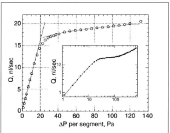
They observed that above a critical applied pressure the flow rate only increases a small amount despite gross increases in the applied pressure (see figure 1-3). This behavior corresponded with the onset of vortex behavior in the solution at a Deborah number of De = 0.8. Such vortex behavior was only observed in polymeric solutions where extensional effect inhibit the flow of the solutions through the contractions. Between a

(18)

range of applied pressures of nearly an order of magnitude (P ~ 20 - 200 Pa), fluid flow rates only increased by a small amount (- 20%). They believed that such a microfluidic resistor could be used as a constant current device that can restrict flow rates despite a wide range of applied pressures.

10

0

0 20 40 60 80 100 120 140

AP per segment, Pa

Figure 1-3. Flow rate dependence on applied pressure drop for the nonlinear resistor proposed by Groisman et al. (Groisman et al., 2003).

In this paper they also detail the mechanism of a "flip-flop" memory device based on polymeric fluid principles. They utilize the difference between the flow of extended polymers with that of relaxed polymers to modify flow patterns within the microfluidic chip. Once again they are taking advantage of the extensional behavior of polymer solutions on the small scale and the subsequent vortex behavior that dictates the flow of polymer solutions (see figure 1-4).

Figure 1-4. Microfluidic flip-flop used by Groisman et al. for controlling flow directions

Again for this study there is little emphasis on the rheological advantages of the fluid and geometries they have chosen. These systems are designed effectively from a functionality

(19)

standpoint, and they have used polymer concentrations that are small enough to keep fluid viscosities near that of water (q - 1.3 mPa-s), however they do not extensively

quantify the rheological properties of their fluids. They suggest that the fluid is in the dilute to semi-dilute range of concentrations but do not determine the possible effects of molecular interaction on flow properties. They also only examine one polymer

concentration, without interpreting the extensional effects of using further diluted solutions of their fluid. Also, the complicated channel geometry leads to asymmetrical vortices, which are not explained in the text. Because no other studies have been performed on similar shapes, there is no explanation for the resulting asymmetry. They also do not quantify the growth of such vortices and whether flow patterns are stable in time or space. Thus, from their results it is difficult to extract any extensive rheological parameters from the flow patterns.

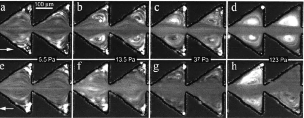
The most recent paper by Groisman and Quake (2004) explains the fundamentals of microfluidic rectifier (a channel whose resistance changes based on the direction of the flow). Once again they use a solution of polyacrylamide (M,= 18,000,000 g/mol) in a Newtonian solvent. The fluid is passed through a series of saw-toothed expansion

contraction geometries. As the Deborah number grows, elastic instabilities develop and flow patterns are no longer reversible (see figure 1-5). Beyond this instability, the fluid acts differently depending on the direction of the flow (see figure 1-6). The extensional behavior is dependent on both the total Hencky strain on the fluid (see section 2.1.3) and the associated strain rate. Based on the geometry the strain should be identical and the strain rate should actually be larger in the direction of the sharper contraction. However, because of the asymmetries in the vortices in the gradual direction, the flow is less stable which translates to a larger amount of total strain in this direction. The more abrupt contraction generates symmetric vortices, which limit swelling at the prior expansion, thus the actual strain is smaller. However this effect is not thoroughly analyzed in their paper.

(20)

Figure 1-5. Streakline patterns for microfluidic rectifier at different applied pressures. Flow travels forward for pictures (a) -(d) and backward for pictures (e) -(h). The images show the irreversibility of the polymer solutions in microchannels caused by elastic instabilities (Groisman and Quake, 2004).

100

Q

10

AP per segment, Pa

Figure 1-6. Flow rate -pressure dependence of the microfluidic rectifier. Circles indicate forward flow (left to right), while squares are backward flow (Groisman and Quake, 2004).

In this paper they accurately describe the transient nature of the vortices as they grow and note that they are steady in the abrupt expansion, but vary with time in the linear

contraction. They also accurately determine the flow rate dependence on the pressure drop over a large range of applied pressures. In each of these papers, they understand the qualitative physics behind their mechanisms, however they do not analyze all the

interacting rheological parameters in a quantitative sense.

-2 ---

---./... _________D ______

(21)

For this paper on the fluidic rectifier, Groisman and Quake characterize the fluid's relaxation time based on an identical polymer concentration in a more viscous solvent, assuming the relaxation time scales with fluid viscosity. However, this estimate does not account for the polymer-solvent interactions, which can have an effect on the measured relaxation time, even in dilute solutions (Brandrup et al., 1975). They also fail to note the

effects of having contraction expansion geometries within such close proximity: the chains may not be able to relax in such a small time, depending on the fluid's velocity. The relaxation times need to be considered in relation to the total residence of the fluid before the next contraction (see section 5.3.3). Because they are attempting to optimize

the polymer stretching on one portion of the channel, it would be advantageous to utilize a hyperbolic contraction (see section 1.6) to generate more uniform polymer stretching. More effective rheological characterization and efficient channel design may allow for extensional effects to increase the magnitude of the nonlinearity of the flow resistance.

These few papers on complex fluids focused primarily on the nature of the flow instabilities and subsequent exploitation of these flow characteristics. From a practical standpoint, it is necessary to understand the rheological nature of such flows before being able to optimize the usage of polymeric fluids in microchannels. Understanding the underlying physics behind the evolution of such vortex behavior and the necessary rheological parameters that dictate the onset of such flow anomalies will ultimately lead to useful applications of such microfluidic devices.

1.3 Entry Flow

Based on the observations of Groisman and others, it is desired to understand the fundamentals behind the elastic nature of fluid flows in microfluidic systems. For many years, understanding and predicting entry flow behavior has been one of the classical problems of fluid mechanics. Entry flow has been a landmark challenge for the experimental, computational, and theoretical worlds (Brown and McKinley, 1994).

(22)

Entry flow has been well quantified for Newtonian fluids, and the results would not be expected to change on the microscale (see figure 1-7). However, for non-Newtonian fluids, where rheological properties change based on the lengthscales involved in the problem, the resulting behavior is not as certain. Polymer solutions are non-Newtonian fluids in which polymers chains exist on at lengthscales of tens to hundreds of

nanometers. Studies have been performed attempting to understand the physics of these fluids on the macroscale (Bird et al., 1987). However, as the lengthscales of the

microchannels begin to approach that of the fluid's microstructure (within an order of magnitude) it is unclear that the behavior of the fluids will continue to mimic that of the macroscale. At such small scales the channels begin to "see" the individual polymers

instead of only bulk fluid.

Figure 1-7. Creeping contraction flow of a Newtonian fluid: comparison of experimental results and computational simulations (Boger et al., 1986).

Entry flow is also a problem with many industrial applications from inkjet printing to microinjection molding (see figure 1-8). Inkjet printing is a high volume commercial industry, which is dependent on extensional flows of a non-Newtonian fluid on the microscale. Micromolding is a growing industry based on scaled-down version of injection molding for which small parts (- 1 ym) can be fabricated by injection of a polymer into a mold through a converging geometry. Naturally, the deficiencies of

injection molding on the macroscale (melt fracture and degradation) still need to be addressed on the microscale. Also, studies have been performed observing the behavior of emulsions passing through contraction for the purposes of flow focusing (see figure 1-9). Microfluidic researchers are frequently concerned with the flow of non-Newtonian

(23)

fluids (especially bio-fluids) in complicated geometries for which shear effects are insufficient in quantifying material behavior (Beebe et al., 2002). Assessing the fluid rheology also requires knowledge of the fluids interaction with stretching. The relevant parameter for characterizing the ability of the fluid to resist stretching is the extensional viscosity.

Figure 1-8. Inkjet printing cartridge: a micro-entry flow of a non-Newtonian fluid

Figure 1-9. Images of a micro-contraction used for flow focusing of emulsions. The contraction is used to generate emulsion droplets (Anna et al., 2003)

1.4 Extensional Viscosity

Just as shear viscosity quantifies the ability of a fluid to resist shearing, the extensional viscosity is a measurement that quantifies the ability of a fluid to resist stretching. The behavior of Newtonian fluids in uniaxial extension is such that its extensional viscosity is

three times its shear viscosity (Trouton, 1906). However, for non-Newtonian fluids there is an additional component to the extensional viscosity that frequently increases the

(24)

extensional viscosity as strain rates increase in an effect termed extensional thickening. The increase in the extensional viscosity is common to non-Newtonian fluids because of their internal microstructure. As the fluid is stretched, these internal elements, which are initially coiled in a random walk, are elongated into a string-like element. This is

especially true in polymer solutions where the polymers are long chains which, when stretched fast enough, exert a large amount of force to prevent further extension.

Typically, at very low strain rates, non-Newtonian fluids act like Newtonian fluids because the fluid relaxes more quickly than it is being unraveled. However, if the fluid is stretched fast enough that the internal microstructure is unable to return to a random walk, extensional thickening takes place. The Deborah number is a comparison of the rate of stretching and the time required for the fluid's microstructure to relax:

De = % (1.2)

where is the strain rate. It has been experimentally and theoretically observed that at Deborah numbers larger than unity, non-Newtonian effects become important (Bird et al.,

1987). Extensional thickening refers to increases in a fluids steady-state extensional viscosity as a function of the strain rate: the onset of which is typically at a Deborah number of unity. Another extensional effect is strain hardening which refers to a transient increase in a fluid's extensional viscosity based on the total strain on the fluid. However,

for entry flows, the strain rates are controlled by the flow rate, whereas the strain is dictated by the contraction ratio. Thus, the extensional behavior of the fluid is dependent on the strain rate.

Previous experiments have shown that for dilute solutions the additional extensional term can be as large as two orders of magnitude greater than the Newtonian extensional

viscosity (Metzner and Metzner, 1970; Spiegelberg et al., 1996; Agarwal and Gupta, 2002; Cooper-White et al., 2002). Most of these experiments however, are limited in their range of strain rates. By working on the microscale, extensional flows can yield

additional information about the fluid properties in regimes beyond what has been

observed in the past. For low viscosity fluids, relaxation times are small enough that non-Newtonian extensional effects only become important at high strain rates.

(25)

Measuring extensional viscosity has been a challenge for experimentalist for many years (Macosko, 1994). For this reason, few extensional rheometers are commercially

available. Several techniques are available for measuring the extensional viscosity

including filament stretching and fiber wind-up. These techniques are generally restricted to low strain rates and high viscosity fluids. There are a few techniques in which it is possible to measure the extensional behavior of mobile fluids (opposed jet being the most common). Figure 1-10 shows the results of an opposed jet study on solutions of

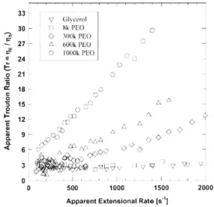
polyethylene oxide (PEO), the same polymer that will be examined in this study (however the solvent viscosities and polymer molecular weights are different). The substantial elastic behavior of these polymers significantly contributes to the extensional viscosity of the solutions. However, in these commercially available techniques, it is not possible to reach the magnitude of strain rates to be examined in this study (see section 5). Using entry flow techniques, mobile fluids can be studied and large ranges of strain rates are readily achievable.

33 V Glycerol 30 - 8k PEO 300k PEO 27 - 00k PEO C 000k PEO 24 o 21 18 C 15 12'( 9 0 0 0 500 1000 1500 2000

Apparent Extensional Rate Is"]

Figure 1-10. Extensional viscosity of various PEO solutions using a opposed jet rheometer

Typically extensional flow problems have been examined on the macroscale. The relevance of moving such observations to the microscale has several implications. First, reducing the size of the geometries allows high strain rates to be achieved:

(26)

iY=k (1.3)

L AL

where V is the average velocity,

Q

is the flow rate, A is the cross sectional area, and L is a characteristic lengthscale. Because the strain rate scales with the inverse of a length scale, at constant velocities, the strain rates in the present experimentation, at moderate flow rates, are several orders of magnitude greater than previous entry flow systems. The obtainable strain rates exceed those achievable on commercial extensional rheometers,

such as the Rheometric RFX opposing-jet rheometer (Hermansky and Boger, 1995; Ng et al., 1996; Cooper-White et al., 2002). Also for previous experiments it was difficult to deal with the inertial effects associated with low viscosity fluids. In microchannels, inertial effects are much smaller, allowing for low viscosity fluids to be examined. Another benefit of using microfluidic devices is their simplicity: microfluidic geometries can be fabricated in a rapid manner and specific to the design requirements (Duffy et al., 1998; Xia and Whitesides, 1998).

One of the drawbacks of using a microfluidic device for measuring extensional properties are that only two-dimensional structures can be generated. This limits the current study to planar geometries, whereas many previous experiments have focused on uniaxial flows (see section 2.1). Another problem with microfluidic systems is that few experiments have been performed trying to make quantitative rheological measurements of these systems. As a result, there has been little emphasis on making sharp vertical sides walls, which is of critical importance to the current project. Another limitation of

microchannels, especially ones fabricated using PDMS (polydimethylsiloxane), as in the rapid prototyping technique (Duffy et al., 1998), is their inability to withstand large pressures. While this is infrequently an issue with low-viscosity fluids, it does become a problem as flow rate and viscosity increase.

1.5 Applications for ISN

The Institute for Soldier Nanotechnologies (ISN) is a United States Army funded project focused on developing technology to improve the quality of soldier apparel. One aspect

(27)

of this project is focused on the development of microfluidic technologies to monitor and control various components of the soldier uniforms. Because the field of microfluidics is relatively new, understanding of many underlying physical phenomena are required for

such devices to become widely used for practical applications.

A great deal of research for ISN has focused on developing field-responsive fluids. These fluids react to external applied fields and subsequently change their mechanical

properties. For example, in the presence of a magnetic field, magnetorheological fluids (MR fluids) change from a mobile fluid to a yield stress fluid. Changing the magnitude of this magnetic field can change the energy absorption by larger than an order of magnitude (Deshmukh, 2003).

One goal of ISN is to produce microfluidic interconnects which will encompass the entire uniform. By integrating valves and pumping systems, these interconnects will allow fluids to travel throughout the uniform as desired to specified locations. By developing pumping schemes such as the ones discussed in section 1.2 (Groisman et al., 2003; Groisman and Quake, 2004), circulation of desired fluids to various portions of the uniform is possible. The significance of this work may allow for the energy absorbing fluids to be transported to various sections of the uniform and subsequently activated in order to protect various areas. These fluids can also be circulated to specific areas of the uniform in order to immobilize a region in the case of injury. Thus, understanding the behavior of these fluids in microchannels is required for determining the optimal configurations required for transporting these fluids.

Based on the magnitude of their energy absorbance, field responsive fluids may also be employed in microchannels to appropriately modify flow conditions. Because of their responsive properties, these non-Newtonian fluids can also be used as valves and

switches for changing flow patterns within microfluidic devices. In figure 1-11 a

switchable microvalve is generated using an MR fluid (5% 500-nm ferrofluid emulsions) that is able to stop the flow of fluid when a field is applied. When the field is released,

(28)

halt the fluid motion completely until a minimum pressure is obtained. This behavior is different from that of the fluids used by Groisman and Quake in which the flow rate was held constant only when pressure exceeded a critical value. The MR fluid is capable of altering the motion of the fluid independently of the applied pressure. In order to use such a fluid to stop flow, it is required to pass the fluid through an extensional flow, so that the fluid can resist acceleration. Optimizing the behavior of such a flow requires an

understanding of extensional nature of a non-Newtonian fluid passing through such devices. For many ISN applications, complex extensional flows of non-Newtonian fluids play an active role in the functionality of microfluidic systems.

Figure 1-11. MR fluid used as a valve to stop fluid flow. Fluid initially flows through channel (left). Upon applying a magnetic field, flow is stopped (right) (image courtesy of Ramin Haghgooie).

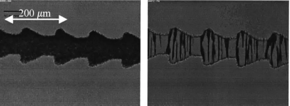
The roughness of the geometries (figures 1-2, 1-4, 1-5, 1-9, and 1-11) in these is another factor that is an important concern in rheology (see section 3.1). Rheological

measurements, especially if they are to be compared to numerical simulations, need to be performed on well-defined geometries.

1.6 Project Goal

The goals of this project are to generate extensional flows in microchannels and quantify the extensional viscosity of dilute polymer solutions. Extensional flows, or shear free flows, are characterized by converging streamlines that indicate stretching of the fluid particles. These flows can be generated through a number of different contractions and

(29)

expansions geometries. Microfabrication limits the choice of geometries to planar shapes. The velocity gradient for a planar pure extensional flow is:

a 1 0 0(

1= I0 -1 0 _(1.4)

ax

\0 0 01/

such that the rate of strain tensor is:

'2 0 0"

V=(Vv+(Vv)T) = 0

-2 0

(1.5)

0 0 _01/

Solving for the flow velocities results in the following two-dimensional flow field:

xIx 2 = xOx20 (1.6)

where the x1 is motion in the direction of the flow, x2 is the motion in the secondary

direction, and x1,o and X2,O are constants for a given streamline. This formula describes a hyperbolic shape for pure planar extensional flow (see figure 1-12). However, this

formula also requires that there is a uniform axial velocity (direction 1) throughout each cross section of the flow. This is difficult to generate in channel flow because of the no-slip boundary condition at the walls. Attempts have been made to lubricate the walls of a hyperbolic geometry to induce slip, but these experiments have generally been

unsuccessful: failing to completely eliminate shear from the flow (Macosko, 1994). Some experiments have been conducted on planar geometries with a linearly converging

geometry (James and Saringer, 1982), but the majority of experiments have been run on abrupt contractions (Walters and Rawlinson, 1982; Evans and Walters, 1986; Evans and Walters, 1989; Chiba et al., 1990; Chiba et al., 1992; Quinzani et al., 1995; Purnode and Crochet, 1996; Ryssel and Brunn, 1999; Olson and Fuller, 2000; Stelter and Brenn, 2000; Nigen and Walters, 2002; Stelter et al., 2002; Mitsoulis et al., 2003). To compare with previous works done on the macroscale, abrupt contractions were chosen as the means of generating extensional flow for the present study (see figure 1-13).

(30)

,-X2

X1'

Figure 1-12. Shear-free planar flow

Figure 1-13. Dimensions of microchannels used in the present study

For entry flow studies, several relevant parameters define the nature of the geometry. The contraction ratio (0p) for a planar geometry is the ratio of the upstream and contraction widths:

W Ac

(31)

where W is the upstream width, W, is the contraction width, and A I and A, are the cross sectional areas of the upstream and downstream contractions. And the aspect ratio (ARp) of the planar channel is defined as:

ARh

AR= (1.8)

W

where h is the height of the channel in the neutral direction. These two dimensionless parameters will be important in comparing the present study with previous entry flow

studies.

In the present study extensional flow properties are examined using several different techniques. The fluid motion is examined using streak image photography to observe the vortex patterns and viscoelastic effects of the extensional phenomena arising near the flow entry. Also, extensional viscosities are calculated using an analysis of the additional pressure loss accrued by the extensional motion of the fluid into the contraction. Before

continuing, it is necessary to examine previous studies conducted using similar

geometries and determine the specific significance of reducing the channel dimensions to the microscale.

(32)

2 Background

2.1 Contraction Experiments

2.1.1 Dimensionless Parameters

In order to compare the results from the present study to that of previous works, both axisymmetric and planar, it is necessary to establish an unambiguous means of

calculating dimensionless variables. The Deborah number is a dimensionless parameter that is indicative of the relative importance of the elastic stresses of the fluid with the timescale of the system (Bird et al., 1987). The Deborah number is defined for a planar contraction geometry as:

De, = 2s = WC (2.1)

and for axisymmetric contractions:

DeA = / (2.2)

R2

where VC is the average velocity in the contraction, We is the characteristic dimension of the planar contraction (as in figure 1-13), and R2 is the contraction radius for an

axisymmetric contraction (see figure 2-1). For Newtonian fluids the Deborah number is zero as there is essentially no relaxation time associated with the fluid. As a Newtonian fluid is deformed, the orientation of the individual molecules change, but they have no preferred orientation, so there is no time scale associated with the dissipation of stresses or relaxation of the microstructure. For polymer solutions, when the fluid is stretched or sheared, the polymer chains extend from their original orientation. However, when the motion is ceased the polymer strands are driven to return to their original random

orientation as a result of entropic forces. This relaxation process takes a finite amount of time, which is based on a number of different factors depending on the specific polymer and the base solvent. The means for evaluating this quantity for the polymer solutions in this study is explained in section 4.3.

(33)

- -- ~1

Figure 2-1. Axisymmetric contraction, as used in previous macroscale studies

Inertia also affects the dynamics of any fluid system. The Reynolds number is a comparison of the relative importance of inertial and viscous stresses in the fluid. The Reynolds number for a planar contraction system is defined as:

Pv W

Re, = C (2.3)

77o

and for an axisymmetric contraction as:

ReA =2pVCR2 (2.4)

7o

where p is the fluid density, 77 is the zero-shear-rate viscosity.

Both the Deborah number and the Reynolds number have an associated lengthscale. Because the present study is performed on the microscale, a comparison of the Deborah number and Reynolds number is greatly affected by this lengthscale. Thus, the elasticity number (El) is used as a dimensionless representation of this comparison:

El, = De- 2117 (2.5)

Rep pW and for an axisymmetric contraction

ElA = (2.6)

2pR2

The elasticity number compares the relative importance of elastic effects in the system with inertial and viscous effects, based solely on channel geometry and fluid properties.

(34)

The magnitude of this parameter is completely independent of the velocity or shear rate of the fluid.

The contraction ratio (0p), is a key parameter in determining the entry behavior for a planar contraction. The contraction ratio is defined as in equation (1.7):

W

We

And for an axisymmetric contraction the contraction ratio is:

I6A = R (2.7)

R2 where R, is the upstream radius.

Non-Newtonian fluids typically possess material properties (namely relaxation time and viscosity) which vary with shear rates (j). These fluids have been used in many similar contraction geometries, but these effects can be accounted for by considering the

rheological properties to be shear rate dependant parameters (Walters and Rawlinson, 1982; Evans and Walters, 1986; Evans and Walters, 1989; Chiba et al., 1990; Chiba et al., 1992; Quinzani et al., 1995; Purnode and Crochet, 1996; Olson and Fuller, 2000; Nigen and Walters, 2002; Mitsoulis et al., 2003). Thus modified dimensionless numbers are also calculated to account for the various effects of shear-thinning and rate-dependent relaxation times. For these non-Newtonian fluids, the elasticity number is no longer independent of the fluid velocity, but the elasticity number does provide a means of comparing the present study with those performed with different fluids and different dimensions.

El(f)- 2/ (2.8)

W"

2.1.2 Entry Behavior

In entry flow problems there is a balance between a number of rheological and inertial stresses that lead to interesting physical phenomena. Various regimes of vortex patterns

(35)

develop and are suppressed based on the relative importance of elasticity and inertia. In an attempt to minimize the total energy consumed in the entry process, flow patterns depart from the simple Newtonian converging flow (see figure 2-2).

Figure 2-2. Vortex growth for a Boger fluid in an axisymmetric contraction (Rothstein and McKinley, 1998).

For the uniaxial case, a number of different regimes have been observed. At low Deborah numbers, a "Moffatt eddy" is observed in the salient corner, as in Newtonian fluids (see figure 2-3). However, for elastic fluids, as the Deborah number is increased, two different vortex patterns are observed. For some fluids, stress singularities at the re-entrant corner lead to a large steady recirculation zone termed a corner vortex (see figure 2-3). The corner vortex typically grows to the re-entrant corner, and a vortex length (L,) is

computed as the reattachment length. The dimensionless vortex length (X) yields another means of evaluating the flow:

- L " (2.9)

W 1PW

At a Deborah number and Reynolds number of zero, the dimensionless vortex length approaches the value for a Moffatt eddy (XhffattA = 0.17 for an axisymmetric contraction

and XIoffattp = 0.19 for a planar contraction (Alves, 2004)). A second regime of fluid

instabilities is termed a "lip" vortex. Here the recirculation is no longer steady in time or space and originates at the re-entrant corner. At higher Deborah numbers both of these vortex patterns become unstable, similar to the melt flow instabilities observed in injection molding of polymer melts.

(36)

Moffatt Eddy Lip Vortex Corner Vortex

~1 LV

Moffatt Eddy _{Re-entrant Corner} _{Salient Comer}

Figure 2-3. Three different vortex regimes observed in axisymmetric contractions

Experimentally, it has been show for axisymmetric contractions that little or no new information is obtained by observing contraction ratios ( 3A) greater than 4. Thus, many

experiments and simulations have been done at this contraction ratio for its practical and theoretical importance. Typically these experiments are also performed using Boger fluids. Boger fluids are fluids with constant viscosity, yet elastic properties. This quality makes them ideal for observing the rheological behavior of many systems.

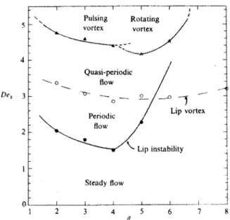
It has been proposed that the nature of elastic behavior for creeping flow in an axisymmetric flow is dependent on the Deborah number and the contraction ratio (McKinley et al., 1991) (see figure 2-4). However this analysis fails to account for the associated inertial stresses that are present in the flow of mobile fluids, as is true for the present experiments.

(37)

Pulsing Rotating vortex vortex 4 Quasi-periodic flow De₂ 3 --n_-O

Periodic Lip vortex

2 0 flo w

Lip instability

0-1

1 2 3 4 flo 5 6 7 8

Figure 2-4. Different vortex growth regimes determined based upon contraction ratio and Deborah number (McKinley et al., 1991).

Based on previous axisymmetric experiments, it appears that the relative importance of elastic and inertial stresses determines which regime of vortex behavior occurs

(especially at a fixed contraction ratio). For this reason the elasticity number is important in quantifying this and previous studies (see figure 2-5). At large elasticity numbers, vortex behavior and significant growth are observed due to elastic stresses. For elasticity numbers less than unity, inertial stresses diminish or completely suppress vortex

behavior. Based on the magnitude of the elasticity number and contraction ratio, it should be possible to predict the subsequent vortex behavior. Because the magnitude of the elasticity number is inversely related to the square of a lengthscale, it is possible to generate large elasticity numbers without using fluids with high viscosity or long relaxation times.