Control of mechanically stable movement
by spinalized frogs
by
Andrew Garmory Richardson
B.S. Biomedical Engineering Case Western Reserve University, 2000
Submitted to the Department of Mechanical Engineering
in partial fulfillment of the requirements for the degree of
Master of Science in Mechanical Engineering
at the
MASSACHUSETTS INSTITUTE OF TECHNOLOGY
June 2003
c
Massachusetts Institute of Technology 2003. All rights reserved.
Author . . . .
Department of Mechanical Engineering
May 9, 2003
Certified by . . . .
Emilio Bizzi
Institute Professor, Professor of Brain and Cognitive Sciences
Thesis Supervisor
Certified by . . . .
Jean-Jacques E. Slotine
Professor of Mechanical Engineering and Information Sciences,
Professor of Brain and Cognitive Sciences
Thesis Supervisor
Accepted by . . . .
Ain A. Sonin
Professor of Mechanical Engineering
Chairman, Department Committee on Graduate Students
Control of mechanically stable movement
by spinalized frogs
by
Andrew Garmory Richardson
Submitted to the Department of Mechanical Engineering on May 9, 2003, in partial fulfillment of the
requirements for the degree of
Master of Science in Mechanical Engineering
Abstract
Evidence suggests that the isolated vertebrate spinal motor system might use only a few muscle synergies for the production of a range of movements. The evolution of such synergies encoded in the spinal cord could be dictated by mechanical stabil-ity requirements for interacting with the environment or by particular performance advantages. Previous work in frogs and cats has shown that the isometric forces measured during movements evoked by intraspinal stimulation converge to a sta-ble equilibrium. In non-isometric conditions, however, there is no guarantee that a similar property of convergence will be observed. We therefore characterized the sta-bility properties of trajectories produced by spinalized frogs. Hindlimb movements in frogs were measured and phasic force perturbations were applied by a Phantom robot (Sensable Tech., Inc) attached at the ankle. EMGs were recorded from 12 hindlimb muscles and used to trigger the perturbations in both hindlimb-to-hindlimb wipes and withdrawals. In both behaviors, we found that the final position of the movements was stable in that the ankle trajectory after perturbation moved to the final position of the unperturbed trajectory. Following deafferentation, wiping movements showed a similar, although weaker, recovery after perturbation. Thus the stability proper-ties found during isometric conditions also hold in dynamic conditions. These results show that spinal neural systems are able to stabilize goal-directed movements. Thesis Supervisor: Emilio Bizzi
Title: Institute Professor, Professor of Brain and Cognitive Sciences Thesis Supervisor: Jean-Jacques E. Slotine
Title: Professor of Mechanical Engineering and Information Sciences, Professor of Brain and Cognitive Sciences
Acknowledgments
I first wish to thank Dr. Matt Tresch for his tremendous encouragement and contri-bution to this project. I furthermore am grateful for the advise and commitment of my advisors, Professor Emilio Bizzi and Professor Jean-Jacques Slotine.
Special thanks go to Russ Tedrake for many helpful discussions and Margo Can-tor for her assistance in this work. Finally, I would like to thank Maura Cahill, Kurt Weaver, and my family for all their support.
Funding for this project was provided by the National Institutes of Health and the Whitaker Foundation.
Contents
1 Introduction 7
2 Methods 13
2.1 Surgical preparation . . . 13
2.2 Experimental setup and data collection . . . 15
2.3 Experimental protocol . . . 16
2.4 Data analysis . . . 18
2.4.1 Kinematics . . . 18
2.4.2 EMGs . . . 20
3 Behavioral characteristics 21 3.1 Hindlimb-to-hindlimb wiping movements . . . 21
3.1.1 Behavioral variability . . . 23
3.1.2 Effects of deafferentation . . . 25
3.2 Hindlimb withdrawal movements . . . 26
4 Movement stability properties 28 4.1 Perturbation characteristics . . . 29
4.1.1 Applied force perturbation . . . 29
4.1.2 Perturbed position . . . 31
4.1.3 Perturbed velocity . . . 34
4.2 Final position stability . . . 36
4.2.2 Hindlimb withdrawal . . . 37 4.3 Trajectory stability . . . 38 4.3.1 Contraction analysis . . . 38 5 Stability control strategy 43 5.1 Kinematic evidence from deafferented frogs . . . 43 5.2 EMG evidence from afferented frogs . . . 46 6 Discussion and conclusion 49
List of Figures
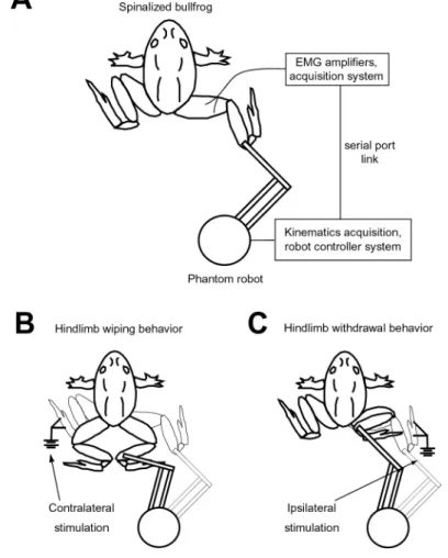
2-1 Schematic of experimental setup and spinal frog behaviors . . . 15
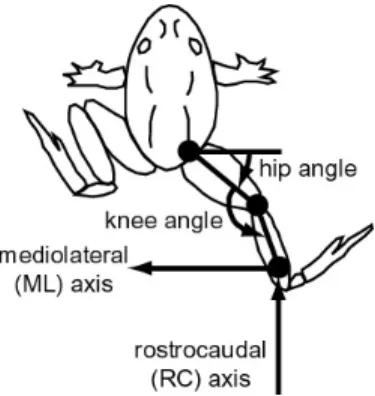
2-2 Coordinate frames for kinematics analysis . . . 19
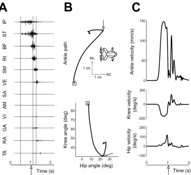
3-1 Example hindlimb wipe motor pattern and kinematics . . . 22
3-2 Mean wiping movements and the biomechanics underlying variability 24 3-3 Afferent influence on wipe motor pattern and kinematics . . . 25
3-4 Example hindlimb withdrawal motor pattern and kinematics . . . 26
4-1 Example hindlimb wipe perturbation trials . . . 30
4-2 Initial displacements for hindlimb wipe movements . . . 32
4-3 Initial displacements for hindlimb withdrawal movements . . . 33
4-4 Perturbed velocities for hindlimb wipe and withdrawal movements . . 35
4-5 Final position summary for hindlimb wipe movements . . . 36
4-6 Final position summary for hindlimb withdrawal movements . . . 37
4-7 Contraction analysis in ankle coordinates . . . 39
4-8 Contraction analysis in alternate coordinates . . . 41
5-1 Perturbation and stability summary for deafferented movements . . . 44
5-2 Example perturbed ankle paths from deafferented frogs . . . 45
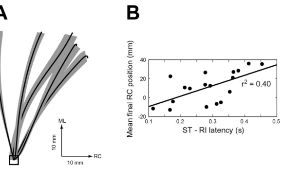
5-3 Relationship between initial and final displacements for wiping move-ments . . . 46
Chapter 1
Introduction
Movement stability is critical for successfully maneuvering about and interacting with the physical environment. The unexpected, or improperly anticipated, presence or absence of a force during motor behaviors can lead to ineffective movement. The huge variety of circumstances under which perturbations can occur, often requiring a quick compensatory response, favors the large majority of perturbations to be han-dled by a rapid stabilizer rather than iteratively through neural learning systems. The neuromuscular system generally acts as the stabilizer of animal behavior, although geometrical and mechanical properties of the skeleton may provide compensation in certain situations [25]. Neuromuscular control can act at several levels to provide sta-bility. First, the neural activation-dependent viscoelastic properties of muscle poten-tially provide passive stabilization at the peripheral level. Second, afferent feedback can drive active compensatory action at the spinal and supraspinal levels. However, nerve transmission delays significantly complicate a stability control strategy relying on supraspinal feedback loops, particularly for high bandwidth movements. In light of this, one might expect a significant reliance on the stabilizing action of peripheral viscoelastic properties and spinal reflexes. In the experiments described in this thesis, we investigate this hypothesis by studying the ability of a spinalized animal, the frog, to recovery from transient perturbations. Subsequently, mechanisms controlling any recovery were explored. We show that movement produced by the frog spinal motor system is stable about behavioral goals and that the stabilization is substantially
provided by the mechanical impedance derived from intrinsic muscle properties. Control theories based on peripheral and spinal stabilizing action
The idea that peripheral properties can stabilize movement has been a central sup-position of several major theories of motor control. Prominent among them is the equilibrium point hypothesis. Originally proposed by Feldman [9], the equilibrium point hypothesis is based on the observation that muscles are better described as spring and damper elements than state-independent force generators. Furthermore, the relationship of muscle length and velocity to force can be modified by motorneuron input [20]. Short-latency spinal reflexes can also add to the total spring-like behav-ior of the neuromuscular system [28], and can likewise be modified by the nervous system. Thus by conceptually simplifying the motor periphery to a set of tunable springs, movement from one point to another may be controlled by changing the rest length of the springs such that the new equilibrium point they define coincides with the desired movement goal. In this way, stabilizing properties of muscles could be used to actually produce movements in essentially the same fashion as a proportional-derivative servo controller for artificial control systems. One of the key benefits of this biological servo control strategy is that, as with its artificial analog, it precludes the need for an inverse dynamics computation and maintenance of a detailed internal model of the motor periphery [30]. In other words, movements can also be imple-mented by the nervous system in terms of kinematic variables (i.e. muscle lengths) and the dynamics of movement naturally emerge from the interplay between stabi-lizing neuromuscular forces and skeletal and environmental loads. Elaborations on this hypothesis have been made, in light of data indicating more than just the fi-nal position of movement is controlled [4], such that a time series of equilibrium points, known as virtual trajectories, may be specified by the neuromuscular system [16]. Also, there has been considerable debate regarding whether desired equilibrium positions are specified by α−motorneuron input, setting intrinsic muscle stiffness (α model [6]), or by γ−motorneuron input, setting spinal reflex threshold (λ model [10]), with the answer likely being some combination of the two [30].
A related theory to the equilibrium hypothesis is impedance control, proposed by Hogan [18]. Extending the concepts of the equilibrium point hypothesis, which utilizes the position-dependent spring-like behavior of the neuromuscular system, this theory unites into a common framework the position-, velocity-, and acceleration-dependent components of mechanical impedance. The nervous system theoretically has a mea-sure of control over both the amplitude and direction of each of these components in the multijoint limb [17]. In particular, muscular redundancy facilitates control of apparent limb stiffness and viscosity while kinematic redundancy of the skeleton is necessary for control over apparent limb inertia. The hypothesis is that the nervous system actively controls each component of mechanical impedance for increased con-trol of limb stabilization. Advantages of impedance concon-trol for multijoint limbs may be realized in tasks where stability is required in certain directions but may hinder performance in others. Experimental evidence suggests that, in some tasks, modula-tion of stiffness [7] and viscosity [26] orientamodula-tion can occur subconsciously. However the ability to voluntarily control all the mechanical impedance components of a limb has not yet been shown [36].
One primary assumption made by both the equilibrium point hypothesis and the impedance control hypothesis is that forces produced by muscle viscoelasticity and spinal reflex action can be made sufficiently large to move the inertial load of the limb and compensate for environmental perturbations. Thus we turn to evidence in the literature exploring the stability properties of the neuromuscular system.
Experimental evidence for peripheral and spinal stabilizing action
To address concerns regarding the magnitude of stabilizing forces produced by in-trinsic and reflex mechanisms, a number of studies have attempted to quantify some or all of the components of mechanical impedance during posture [31] [8] [42] and movement [3] [13] in humans. Impedance was generally determined by applying a controlled force or displacement perturbation, measuring restoring forces, and fitting the mechanical response to a parametric or nonparametric [35] model. Interpretation of the significance of impedance values varied across studies. Generally, stiffness
dur-ing movement was found to differ from posture, but the resultdur-ing impedance values were dependent on a simplified model of the neuromusculoskeletal system. A model-independent study simply inferred from physical principles that the restoring force direction to a constraint perturbation had a large position-dependence, thus provid-ing sprprovid-ing-like stability [43]. Two recent human studies have taken yet a different approach to determining the influence of the spring-like nature of the neuromuscular system on movement stability. Both employ a kinematic, rather than impedance or restoring force, characterization of stability, while ensuring subjects did not make voluntary corrective movements following the perturbation. The first study applied phasic force perturbations during small amplitude, point-to-point movements and found that the final position was not achieved by the subjects [37]. The second study loaded nominal wrist movements and then perturbed the movements by unloading the movement [14]. As with the previous experiment, the final position was not achieved in perturbed trials indicating intrinsic and reflexive actions may not be sufficient to compensate for perturbations, casting doubt on their role as servo controllers.
In addition to the human studies, a separate line of experimental investigation has been pursued in the frog and cat that relates to the nature of stabilizing forces or-ganized by spinal motor circuits. In these experiments, intraspinal microstimulation was applied and isometric forces of the hindlimb were recorded with the limb in vary-ing configurations [12] [27]. For a given spinal stimulation site, ankle isometric forces at each limb configuration pointed toward a particular point in the workspace, thus specifying a convergent force pattern. This arrangement of force directions would be expected to stabilize the limb about a particular configuration. A relatively small number of different patterns were found to exist [5]. Finally, when two spinal sites corresponding to two different patterns where stimulated simultaneously, the result-ing force pattern was a vector sum of the force pattern associated with stimulatresult-ing each site independently [32]. The linear combination of a small number of force pat-terns was interpreted as a possible mechanism for simplifying control, by reducing the excess degrees of freedom provided by the redundant musculature. The stability prop-erties of the force patterns may suggest that some structure embedded in the spinal
cord can coordinate specific combinations of intrinsic muscle properties and reflex loops into stable functional units. These stable units, or primitives, could perhaps be used in a servo control strategy based on ankle position rather than individual muscle lengths. However, data from the human experiments suggests that stability seen in posture does not necessarily translate into stable movement. Indeed, studies have found instabilities in movement deprived of any voluntary corrections [37] [14]. Thus the stabilizing ability of these spinal primitives seen in isometric conditions many not hold in movement of the frog or cat hindlimb.
The experiments described here extend this previous work in the frog, assessing the dynamic stability of movements. The results of this study are both specifically applicable to frog and cat intraspinal stimulation experiments, as well as generally to the ability of peripheral and spinal mechanisms to stabilize movement in the absence of supraspinal control.
Outline of chapters
Chapter 2 describes the methods employed in carrying out the frog experiments, in-cluding surgery, experimental setup, data collection and analysis.
Chapter 3 provides a brief description of the nominal behaviors elicited from the spinalized frog, discussing the variability observed across and within frogs as well as the effects of deafferentation on the basic motor pattern.
Chapter 4 gives the main stability results. The commanded perturbations are de-scribed and their effect on the hindlimb kinematics is quantified. Stability about the final limb position is determined. A tool from nonlinear systems analysis, contraction analysis, is applied to determine stability of the full trajectories.
Chapter 5 presents an analysis of the controller stabilizing the system. Intrinsic and reflex mechanisms are differentiated using an EMG analysis and results from
deafferented frogs.
Chapter 6 discusses the results in the context of the background presented in this chapter.
Chapter 2
Methods
2.1
Surgical preparation
All procedures were approved by the Committee for Animal Care at MIT. 40 adult bullfrogs (Rana Catesbiana) were used in these experiments. Animals were anes-thetized with a combination of tricaine (5% solution, 0.5-0.7 ml) and ice anesthesia. The skin overlying the skull was opened, and the muscle tissue overlying the foramen magnum between the first vertebra was removed. The foramen magnum was opened and the skull overlying the tectum and brainstem was removed. The dura was opened and the exposed spinal cord aspirated at the caudal margin of the fourth ventricle, completely separating the spinal cord from the brainstem. All neural tissue rostral to the brainstem was then removed by aspiration and the remaining cranial cavity was packed with gelfoam to minimize bleeding. Gelfoam was also placed over the exposed spinal cord and brainstem and the wound was close using staple sutures.
Animals were then implanted with bipolar electromyographical (EMG) electrodes. Electrodes were constructed from braided stainless steel wires, insulated with Teflon. (7 strands, 0.023 mm). Pairs of wires were knotted together at one end and the knot covered with modeling wax to insulate the two cut ends, forming a wax ball at the end of the electrode pair. The Teflon insulation covering each wire was then stripped for a length of ≈ 1 mm, separated from the wax ball by a distance of ≈ 1-2 mm. The wires were then inserted in the muscle, so that the stripped regions of the
elec-trode pair were located inside the muscle belly with the pair secured by the wax ball. The orientation of the electrode pair was parallel to the orientation of the muscle fibers. The following muscles were implanted: semitendinosus (ST), sartorius (SA), rectus internus (RI), adductor magnus (AM), vastus internus (VI), semimembranosus (SM), vastus externus (VE), biceps femoris (BF), iliopsoas (IP), rectus anterior (RA), tibialis anterior (TA), and gastrocnemius (GA). EMG electrodes were tunneled sub-cutaneously to an exit point on the back and attached to a connector strip.
The dorsal tibia just proximal to the ankle was then exposed. Two bone screws were placed in the tibia, dental cement poured around them, and a vertically oriented threaded attachment placed in the cement. The attachment was used to couple the frog hindlimb to the robot during experiments (see below).
In some frogs (8) we also performed a deafferentation. For this procedure, we ex-posed the spinal cord by dorsal laminectomy of the 6th vertebra. The dura overlying the spinal cord was opened by bipolar electric cautery. In initial experiments, the 7-9th lumbar spinal dorsal roots were identified by the lack of motor response observed following electrical stimulation with silver hook electrodes placed around each nerve. In later experiments, these dorsal roots were identified visually. After identifying the dorsal roots and bathing the exposed spinal cord in tricaine, the dorsal roots were cut. We observed no motor response on cutting the roots, even though animals were usually reflexive prior to bathing the exposed spinal cord in anesthetic, suggesting a lack of injury discharge following sectioning of dorsal roots. Gelfoam was placed on the exposed spinal cord, and the wound was closed in layers, suturing the muscles and then the skin together. Completeness of the deafferentation was confirmed the following day by the absence of all motor responses evoked from scratching sites on the deafferented hindlimb.
Following these procedures, animals were placed in a refrigerator and allowed to recover overnight.
2.2
Experimental setup and data collection
The following day, animals were placed on a stand and secured by a clamp placed around their pelvis. The hindlimb was attached to a Phantom 1.0 robot (Sensable Technologies) using the threaded attachment cemented to the tibia as the point of at-tachment (Fig. 2-1A). This atat-tachment point between the robot and the animal was adjusted so that the frogs ankle was placed in the plane of the hip. The movement of the hindlimb was restricted to this plane by the robot. These restrictions allowed the hindlimb configuration to be determined uniquely from the endpoint of the robot.
Figure 2-1: Schematic of experimental setup and spinal frog behaviors
A pair of stimulating electrodes was placed on the skin of the foot to evoke either hindlimb-hindlimb wipes or withdrawal behaviors in the limb. Hindlimb wiping in the limb attached to the robot was evoked by placing the stimulating electrodes on
the limb contralateral to the attached limb (Fig. 2-1B). Withdrawal was evoked by placing the electrodes on the limb attached to the robot (Fig. 2-1C).
In hindlimb wipes, electrical stimulation evoked a movement of both the stim-ulated hindlimb and the hindlimb attached to the robot toward the midline (see Chapter 3). To prevent the two hindlimbs from colliding and affecting the measured kinematics, we placed a barrier near the animal’s midline. This barrier guaranteed that on repeated wipes, the trajectory of the measured hindlimb was not affected by the contralateral leg.
Activity on EMG electrode pairs was differentially amplified (x1000) and filtered (10-10000 Hz passband, A-M systems) and sampled at 1000 Hz using Labview soft-ware (National Instruments). Kinematic data and the forces applied to the hindlimb attached to the robot were measured on a computer running custom software written using the Ghost software package (Sensable Technologies). Kinematic and force data were collected at 1000 Hz. All data was saved for offline analyses.
2.3
Experimental protocol
We examined the trajectories and EMG patterns produced in hindlimb wiping and in withdrawal behaviors. In all cases of hindlimb wiping, the trajectory and EMG activity of only the unstimulated, wiping, limb was measured. For both behaviors, we examined trajectories in unperturbed trials and in trials in which a phasic pertur-bation was applied.
For unperturbed trials, a behavior was evoked by electrical stimulation applied to either the ipsilateral or contralateral foot. The trigger for stimulation onset was given by the computer running the robot software. This trigger was also used to initiate data collection on the EMG computer. In separate experiments using an external clock sent to both computers, we found that there was constant 3 ms delay between the trigger sent by the Phantom and the start of EMG data collection, with no vari-ability in this delay over repeated triggers. This delay was subtracted in all data sets to align EMG and kinematic data. Electrical stimulation consisted of trains of
bipha-sic stimulus pulses (train duration: 600-1700 ms, train frequency: 25-35 Hz, pulse duration: 1-2 ms, pulse amplitude: 1-1.8 mA). Intervals of 2-5 minutes were allowed between repeated stimulation trains, so as to minimize habituation or potentiation of behaviors. Kinematic and EMG data were recorded for a period of 4 s following the onset of the electrical stimulation.
For perturbed trajectories in both wipes and withdrawals, the onset of the per-turbation was triggered from the observed EMG pattern. This trigger based on EMG activity was used rather than one based on a fixed time following stimulation onset in order to ensure that the perturbation was applied at a similar time in the evoked motor behavior. Perturbations were applied early in the evoked motor pattern, usu-ally within the first 100 ms of the EMG activity. Several observations suggest that the sensitivity of frog hindlimb movements to perturbations is especially high during the early phases of movement production [34]. Perturbations applied early should therefore have the highest probability of evoking measurable compensations in ob-served behaviors. Integrated EMG from the earliest activated muscle (ST, BF, or IP; determined for each frog individually) was measured online in 5 ms bins and accumu-lated until it crossed a threshold. When this threshold was crossed, a perturbation was applied to the frog hindlimb. The threshold was chosen for each frog so that the perturbation was triggered within the first 100 ms of observed EMG (see Fig-ure 4-1A) but was insensitive to baseline noise. Perturbations were applied in two different directions, defined with respect to the instantaneous velocity of the ankle. Clockwise (CK) perturbations were applied at an angle of +90 to +135 degrees while counterclockwise (CCK) perturbations were applied at an angle of -90 to -135 degrees. CK perturbation trials, CCK perturbation trials, and unperturbed trials (O), make up the three perturbation groups referred to in the data analysis. The perturbation command consisted of a square pulse, amplitude 0.35 to 1.50 N and duration 25 to 75 ms. We confirmed the peak amplitude and duration of the perturbation in sep-arate experiments using a force transducer attached to the robot. Care was taken so that the applied perturbation did not drive the limb into the boundaries of the frogs workspace, which could be observed by a clear and immediate return of the
hindlimb to the unperturbed trajectory following the perturbation. Any such trials were excluded from further analysis.
2.4
Data analysis
All analyses of kinematic and EMG data were performed using MATLAB software (MathWorks).
2.4.1
Kinematics
The perturbed kinematics of the hindlimb wipe and withdrawal behaviors were used to determine stability. To prepare the kinematics for analysis, the goal-directed por-tion of the hindlimb trajectories was determined using criteria similar to that used in [38]. For hindlimb wipes, the portion of the observed trajectory up until collision with the midline barrier was identified. For withdrawal reflexes, the portion of the observed trajectory up until collision with the body of the frog was identified. Be-sides observing the trajectory reaching the boundaries of the hindlimb workspace, these collision points could be seen in a sharp transient of the hindlimb velocity pro-file. These collision points were considered to be the end of the movement for the purposes of the subsequent analyses.
Prior to the stability analyses, the degree to which the perturbation caused a change in hindlimb kinematics was quantified. Perturbed position was measured relative to the unperturbed mean path. To calculate this path, the path of each in-dividual unperturbed trajectory was spatially resampled, using spline interpolation, such that there was an equal distance between each point along the path from initial to final position. The resampled paths were then averaged, point by point, to obtain the mean unperturbed path. The variance and 95% confidence intervals of this mean path were calculated from these same distributions of resampled trajectories. The initial displacement due to the perturbation was taken as the maximum displacement from the mean unperturbed path, calculated along directions perpendicular to the path, in the 100 ms following perturbation offset. This time window included the
pe-riod of time during which the hindlimb was still moving away from the unperturbed path after the initial acceleration caused by the perturbation. For reference, this distance was also calculated for unperturbed trials, where time of perturbation off-set was determined using the same EMG threshold criterion of when a perturbation would have been applied. Initial displacements were also analyzed in the joint space of the frog hindlimb. For this analysis, we used link lengths measured from x-rays taken post mortem and measurement of the frog’s hip position to transform the ankle positions of the hindlimb to joint coordinates (as defined in Figure 2-2). In addition
Figure 2-2: Coordinate frames for kinematics analysis
to perturbed position, the effect of the perturbation on limb velocity was assessed in both joint space and muscle space. For the latter, we used a detailed biomechanical model of the frog hindlimb developed by Bill Kargo and Larry Rome [23]. Using the configuration-dependent moment arms of ST and BF provided by this model, along with the joint velocities calculated from the observed trajectories, we obtained an estimate of the velocity of muscle lengthening or shortening caused by the applied perturbations.
Two stability analyses were performed using the kinematic data. The first com-pared the final position of unperturbed trials to that of perturbed trials to test sta-bility about the final position. The second tested the tendency for each pair of CK and CCK perturbation trajectories to converge towards each other, using contraction analysis [29].
2.4.2
EMGs
EMGs were analyzed primarily for the purpose of determining the role of spinal re-flexes in compensating for the phasic perturbations. All EMGs were rectified and then digitally filtered (acausal 5th order low pass Butterworth filter, 20 Hz nominal cutoff). Onsets and offsets of muscle activations were determined using an automatic detection routine. These values were verified visually for each trial and adjusted when necessary. For a qualitative analysis of EMG alterations following the pertur-bation, mean EMGs were computed for each perturbation group of each frog after aligning the EMGs of each trial on perturbation onset. For the unperturbed group (O), trials were aligned on when the perturbation would have occurred, using the same EMG threshold criterion mentioned above. For a statistical analysis of EMG alterations following the perturbation, we looked at perturbation group differences in three parameters: latencies between onset of different muscles, duration of individual muscles, and magnitude of individual muscles. The duration of EMG response was taken as the time from onset to offset of each muscle. The magnitude of each muscle activation in a trial was calculated as the total integrated EMG for that muscle from perturbation onset to time of final position as defined by the kinematics. Of the six frogs comprising the withdrawal movement data set, two had poor ST or BF EMGs and thus were excluded from all EMG analyses. Each test was performed using a non-parametric Kruskal-Wallis ANOVA.
Chapter 3
Behavioral characteristics
This chapter briefly describes the typical motor patterns and kinematics of nominal, i.e. unperturbed, hindlimb wipe and withdrawal behaviors. Variability in the nominal motor patterns is analyzed to identify some features that can be modulated by the spinal circuits involved in these behaviors. The role of afferent feedback in modulating these features is also described. Changes in the relevant motor pattern parameters identified in this chapter are later considered, in Chapter 5, as possible afferent-driven stabilizing mechanisms.
3.1
Hindlimb-to-hindlimb wiping movements
The primary spinal frog behavior used in this thesis is the hindlimb-to-hindlimb wipe (referred to henceforth as hindlimb wipe or wipe). Previous investigations have used this behavior as a tool for studying sensory to motor mappings and controlled move-ment variables by vertebrate spinal circuits [11] [38]. The behavioral goal is to use the ankle of one hindlimb to wipe off an irritating stimulus on the other hindlimb (Fig. 2-1B). A particular advantage of this behavior is that it demands relatively precise multijoint movement to remove the stimulus, presumably requiring more so-phisticated neural control than ballistic movements such as kicking or withdrawal.
A typical example of the motor program, as determined from EMG activity, and kinematics of a hindlimb wipe is shown in Figure 3-1. The degree of sophistication
Figure 3-1: Example hindlimb wipe motor pattern and kinematics
of the movement can perhaps be seen most clearly in the staggered, rather than syn-chronous, EMG activity of hindlimb muscles (Fig. 3-1A). The muscle activity can be divided into three phases, as roughly demarcated by the vertical lines: an initial phase involving predominantly knee flexors (IP, ST, BF), a second phase involving predom-inantly hip extensors (RI, SM), and a final phase involving a knee extensor (VE) as well some muscles acting at the ankle joint (GA, RA, TA). The putative biomechani-cal action of the muscles just described is in agreement with the joint kinematics (Fig. 3-1B). From the initial position, indicated by the square, the first part of the move-ment is dominated by knee flexion, followed by hip extension, and ends with knee extension (refer to Figure 2-2 for sign convention of joint angles). In ankle
coordi-nates, the first two phases of muscle activity correspond to a rostral-medial movement toward the midline to place the two limbs in contact with each other (the RC and ML axes arrows point rostral and medial, respectively, as indicated by orientation of the inset frog). Thus the first two phases are referred to collectively as the placing phase in this thesis. This is followed by a caudal extension of the limb contralateral to the stimulus to wipe off the irritating stimulus on the other limb, referred to as the whisking phase [11]. The velocity profiles in joint and ankle coordinates are fairly monophasic for the placing phase of the movement (Fig. 3-1C). A sudden decrease in velocity occurs upon contact with midline barrier (see Section 2.2), followed by a distinct velocity peak for the whisking phase. These characteristics of the wiping behavior are essentially the same as those reported in previous studies [21] [22].
For the purpose of evaluating stability properties, the placing phase of the hindlimb wipe movement is of most interest. This phase has a well defined final position, namely the point approximately along the midline of the frog where the wiping limb makes contact with the midline barrier, making it similar to point-to-point movement tasks often used in evaluating stability properties in humans [37] [43]. One difference, how-ever, is that the velocity is generally nonzero at the final position of the placing phase. To isolate the placing phase, as mentioned in Section 2.4.1, kinematic records were truncated at the point of midline contact (indicated by an arrow in Figure 3-1).
3.1.1
Behavioral variability
Variability in the placing phase of the wipe is largely manifest in the rostrocaudal position along the midline at which the contralateral limb makes contact. Mean unperturbed ankle paths and 95% confidence intervals on the mean (assuming a Student’s T distribution) are shown for five frogs in Figure 3-2A. Across different frogs, or different recording sessions in the same frog (16 frogs, 18 sessions for the combined set of afferented and deafferented wiping behaviors), the mean final rostrocaudal position had a range of 48.8 mm. However within a recording session of a given frog, the unperturbed paths were fairly consistent with a mean range of 9.9 mm.
Figure 3-2: Mean wiping movements and the biomechanics underlying variability could be related to changes in the EMG patterns. Nine relationships were tested: RC final position as a function of five muscle magnitudes (IP, ST, BF, RI, and SM; magnitude defined as in Section 2.4.2) and as a function of four onset latencies between muscles (ST-RI, ST-SM, BF-RI, and BF-SM). These EMG parameters were chosen due to their relevance in the behavior as identified above and in previous studies [21] [22]. The final rostrocaudal position variability between the 18 hindlimb wipe data sets could in large part be accounted for by the latency between knee flexor and hip extensor muscle activity of the placing phase (Fig. 3-2B). In particular, the latency between onset of ST and onset of RI was significantly correlated to the mean final rostrocaudal positions (p < 0.005) and accounted for 40% of the position variance. Shorter latencies, i.e. longer RI contributions to the movement, correspond to caudal final positions while longer latencies, i.e. less RI contribution, lead to more rostral positions. This relationship is consistent with the biomechanics, as longer latencies allow knee flexor torques to drive most of the movement to the midline, bringing the ankle more rostral. The other eight EMG parameters were not significantly correlated with final RC position in these data sets.
3.1.2
Effects of deafferentation
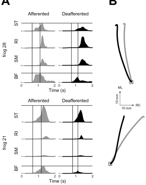
Deafferentation of the spinalized frogs provided a means of separating the reflex and intrinsic, i.e. muscle viscoelastic, contributions to movement stabilization. However we also found that deafferenation modifies the nominal behavior, as described in [21]. Of the eight frogs that were deafferented, two underwent testing both in the afferent and deafferented conditions. The knee flexors (ST,BF) had a decreased amplitude
Figure 3-3: Afferent influence on wipe motor pattern and kinematics
3-3A, EMGs have been rectified, filtered, aligned, and averaged across trials). Both of these observations are consistent with a more caudal mean final ankle position in the deafferented animal (Fig. 3-3B). These observations are also consistent with a recent quantitative analysis of afferent influences on hindlimb wipe behaviors of spinalized frogs [21].
3.2
Hindlimb withdrawal movements
In addition to the 16 spinal frogs used to study hindlimb wiping movements, seven frogs were used to test the stability properties of hindlimb withdrawal movements. The goal of hindlimb withdrawal behaviors is to quickly move the hindlimb away from
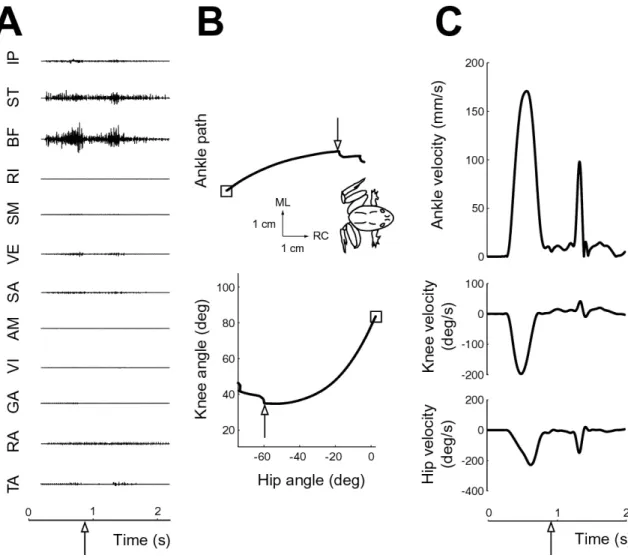
an aversive stimulus (Fig. 2-1C). Withdrawals are more of a ballistic movement than hindlimb wipes, involving synchronous activity of the flexor muscles: IP, ST, and BF (Fig. 3-4A). These muscles both cause flexion of the knee and hip, moving the ankle in a rostral-medial direction until contact is made with the body (Fig. 3-4B). Like the placing phase of the hindlimb wipe, velocity profiles are monophasic up to the point of contact (Fig. 3-4C). For the stability analysis, the final position for this behavior is defined as the point at which the ankle first touches the body (indicated by an arrow in Figure 3-4).
The characteristics of the nominal wipe and withdrawal behaviors observed in our experiments are consistent with those found in previous studies [21] [22] [38]. We found that variability in the wipe movements, as parameterized by final rostrocaudal position, can be significantly correlated with the latency between the onset of ST and RI activity. Furthermore, this latency is modulated by afferent feedback, as deter-mined from the changes in motor patterns following deafferentation. Thus we can hypothesize that changes in ST-RI latency may contribute to perturbation compen-sation in the wipe, although the other afferent-driven contributions will be tested in Chapter 5 as well.
Chapter 4
Movement stability properties
The ability of the spinal frog to compensate for perturbations during hindlimb wipe and withdrawal movements is examined in this chapter. First, the phasic pertur-bations that were applied to the hindlimb by the Phantom robot are characterized in terms of the extent to which they changed the kinematics of the limb relative to unperturbed trials. This characterization is used to indicate whether the perturbed kinematics exceeded the variability of the movement, a necessary condition for in-ferring any subsequent compensation. The analysis can also suggest whether these kinematic changes could be sensed by the frog proprioceptive system, based on known sensitivity of frog muscle spindles. This is an important consideration for the next chapter, which explores the stabilizing strategy employed by the spinal frog. Second, stability is assessed in terms of both final position and trajectory. The assessment of the latter utilizes contraction analysis, a tool from nonlinear systems theory that tests for a type of stability particularly amenable for a system to be embedded in or a result of a distributed control architecture.
4.1
Perturbation characteristics
4.1.1
Applied force perturbation
The onset of phasic perturbations of the hindlimb movements was triggered when a threshold IP, ST, or BF EMG activity was exceeded. As shown in the last chapter, these muscles generally were the first activated in both wipe and withdrawal move-ments. Since the stability analysis employed in this thesis is based on the kinematics, rather than restoring forces or impedances, timing the perturbations relative to these muscles allowed the perturbations to occur sufficiently early in the movement to de-termine whether the perturbed kinematics tended toward the unperturbed kinematics prior to midline (wipe) or body (withdrawal) contact. The EMG-based perturbation timing also ensured that muscles were active at the time of the perturbation, thus increasing the likelihood that muscle spindles would sense the perturbation. This rationale is valid for the frog since it does not have independent alpha and gamma motor neuron drive, unlike higher vertebrates, but rather a beta system which cou-ples efferent activity to extrafusal and intrafusal muscle fibers. Finally, EMG-based perturbation timing improved the consistency of the perturbation, implementing the perturbation at approximately the same point in the motor program from trial to trial. An example of this consistency is shown in Figure 4-1A. The EMGs for two perturbation trials of hindlimb wiping movements are shown, both aligned to stim-ulation onset. The vertical bar indicates the perturbation onset, as triggered by IP activity, and duration. The second perturbation trial shown had a slightly longer latency from stimulus onset to motor response than the first, but due to the EMG-based triggering the perturbations occurred at the same point in the motor pattern. The direction of the applied perturbation was either 90-135 degrees clockwise (CK) or counterclockwise (CCK) to the ankle movement direction at the time of perturbation onset. These directions permitted the spatial characterization of the perturbation effect, i.e. displacement from the mean unperturbed path, rather than the temporal measures a purely assistive or resistive perturbation would likely re-quire. Example CK and CCK perturbed paths, in ankle and joint coordinates, are
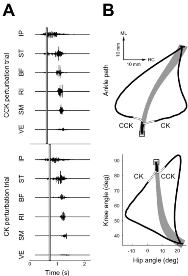
Figure 4-1: Example hindlimb wipe perturbation trials
shown in Figure 4-1B with initial position indicated by a square. The portion of the path where the force perturbation was applied is indicated in white. The grey region indicates the 95% confidence interval for the unperturbed mean path. The maximum displacements from the unperturbed mean path in these examples are substantial, approximately one-third to one-half of the total ankle path length. In these exam-ples, a full recovery is made back to the unperturbed mean, indicating the placing phase of these wiping movements is stable about the final midline position.
The magnitude of the applied perturbation ranged from 0.35 to 1.50 N and the duration ranged from 25 to 75 ms. For the example in Figure 4-1, the applied force was 1.25 N for 25 ms. These brief and relatively large perturbations rapidly changed
the mechanical state of the limb (position and velocity) in a manner analogous to changing initial conditions of a dynamic system with a delta function input. Upon perturbation offset, acceleration- and possibly velocity-dependent inertial forces carry the multijoint hindlimb further from the unperturbed path before compensating forces dominant the motion. No gravitational forces are involved since these movements are restricted to the horizontal plane.
4.1.2
Perturbed position
The effect of the perturbation on the position of hindlimb movements was analyzed to assess the statistical and functional significance of the perturbation. The initial displacement due to the perturbation was defined as the maximum displacement from the mean unperturbed ankle path, calculated along directions perpendicular to the path, in the 100 ms following perturbation offset.
Afferented hindlimb wipe
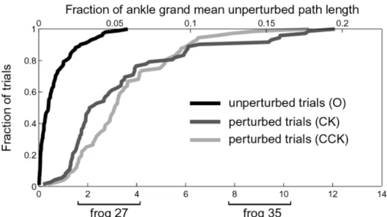
The cumulative distribution of initial displacement for all trials of all eight frogs for the afferented hindlimb wipe condition is shown in Figure 4-2A (109 O unperturbed trials, 85 CK perturbed trials, 105 CCK perturbed trials). The difference between pertur-bation group (O, CK, CCK) distributions is highly statistically significant (pairwise Kolmogorov-Smirnov tests, all p << 0.001) indicating the perturbations exceeded the variability of the movement. The upper abscissa gives a measure of the functional significance of the perturbed position, relating it to the fraction of the total unper-turbed path length averaged across all eight frogs. The clockwise (CK) perturbations tended to cause less of a displacement than counterclockwise (CCK) trials. This may be due to anisotropy of the apparent ankle impedance, a phenomenon associated with multijoint limbs [17].
The initial displacement in joint coordinates (calculated using the same method as for ankle coordinates) is given for two of the eight frogs (Fig. 4-2B): one (Frog 21) that had small to moderate ankle initial displacement and one (Frog 19) that had
Figure 4-2: Initial displacements for hindlimb wipe movements
large ankle initial displacement. For both frogs, the perturbations caused a larger change in hip angle than knee angle. For frog 19, the change in hip and knee an-gle was the same sign: both extension (positive) for CCK perturbations and both flexion (negative) for CK perturbations. For frog 21, the change in hip and knee angle differed in sign. The fraction of joint angle change to mean unperturbed joint movement, a measure of the functional significance of the perturbed joint position, is indicated on the right ordinate.
Hindlimb withdrawal
The cumulative distribution of initial displacement for all trials of all six frogs for the hindlimb withdrawal condition is shown in Figure 4-3A (101 unperturbed trials, 72 CK perturbed trials, 72 CCK perturbed trials). As with the wiping movements, the
Figure 4-3: Initial displacements for hindlimb withdrawal movements
difference between perturbation group distributions was highly statistically significant (pairwise Kolmogorov-Smirnov tests, all p << 0.001), again indicating the perturba-tions exceeded the variability of the movement. Overall, the initial displacements in the withdrawal (middle 50th percentile range for CCK perturbed trials: 2.07 mm
to 4.99 mm) were smaller than for the wipe (middle 50th percentile range for CCK perturbed trials: 4.02 mm to 8.21 mm). This difference is at least partially a result of smaller force perturbation magnitudes applied to withdrawal movements (mean = 0.53 N) as compared to wiping movements (mean = 0.62 N). Like the wiping move-ments, there was some tendency for CK perturbations to cause less displacement than CCK perturbations, suggesting a directionality to the ankle impedance function.
The initial displacement in joint coordinates for withdrawal movements is given for two of the six frogs (Fig. 4-3B). The two frogs are representative of the total ankle perturbation position range. In contrast with the wiping movements, perturba-tions to withdrawal movements caused approximately the same amount of deviation in knee angle and hip angle and the sign of the hip and knee angle changes differed.
Thus the perturbations to both hindlimb wipe and withdrawal behaviors caused the path of the hindlimb to significantly deviate from unperturbed paths. To extend this analysis of the effect of applied perturbations on hindlimb kinematics, changes in hindlimb velocity are considered in the next section.
4.1.3
Perturbed velocity
In looking at perturbation-induced changes in hindlimb velocity, the particular fo-cus was to determine the likelihood of muscle spindle response. Studies in humans have found that as change in joint velocity following a perturbation increases, reflex-ive response to the perturbation is suppressed [41]. Therefore rather than present velocity changes in ankle coordinates, to facilitate an estimate of spindle response the velocities are expressed in joint and muscle (ST,BF) coordinates. Perturbation induced velocity changes were analyzed for the same two pairs of frogs used to exam-ine perturbed joint positions in the previous section. Velocity profiles for each trial were aligned by perturbation onset and averaged for the first 200 ms following onset. Within this time window the velocity profiles were relatively consistent across trials and exhibited the major velocity changes. The transformation from joint to mus-cle coordinates used musmus-cle-specific, configuration-dependent moment arms found for
Rana pipiens by Kargo and Rome [23], scaled up by ratio of tibiofibula length for the bullfrogs used in this study.
Perturbed velocities for both wipe (Fig. 4-4A) and withdrawal (Fig. 4-4B) move-ments exhibited a tendency to oscillate about the unperturbed velocity, rather than returning monophasically. Changes in muscle velocity following perturbation did not exceed 20 mm/s. This is well within the dynamic range of spindle response and, according to results from Ottoson [34], would be expected to cause a spike frequency change on the order of 20 impulses per second over basal, unperturbed levels. Note
Figure 4-4: Perturbed velocities for hindlimb wipe and withdrawal movements that in Figure 4-4 muscle shortening velocities are positive while lengthening is neg-ative and perturbation groups (O, CW, CCW) are indicated by the same colors as in
Figures 4-2 and 4-3.
The perturbed position and velocity achieved in both hindlimb wipe and with-drawal movements substantially exceed the variability in the unperturbed movement, likely making recovery from the perturbation behaviorally relevant and allowing an analysis of any such recovery. Also, the perturbation caused kinematic changes to which muscle spindles should be capable of responding. The rest of this chapter presents a kinematic analysis of the perturbation recovery.
4.2
Final position stability
4.2.1
Hindlimb wipe
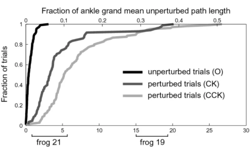
Stability about the final hindlimb position was analyzed across the eight afferented wiping frogs by examining the cumulative distributions of unperturbed and perturbed trial final position distances from unperturbed mean final position (Fig. 4-5). Pairwise Kolmogorov-Smirnov tests found no pair of distributions that significantly differed (p > 0.1 for all three tests), indicating that the perturbed trial final positions where indistinguishable from unperturbed trial final positions. The magnitude of recovery
can be seen by comparing the cumulative distributions in Figure 4-5 to those in Figure 4-2A. As a within session (8 frogs, 9 sessions) test of final position stability, a one-way multiple analysis of variance (MANOVA) on the final positions for the three groups of trials found six out of the nine sessions showed no significant difference in final position at the α = 0.05 level (using the Wilks’ lambda test statistic which has an exact F distribution for two dependent variables and three groups, see Johnson and Wichern [19]). All three sessions with a significant main effect had a significant pairwise effect between unperturbed trials and CCK perturbed trials at the α = 0.05 level (using Bonferroni method of familywise significance adjustment for multiple tests).
4.2.2
Hindlimb withdrawal
Stability about the final position in withdrawal movements was comparable to that of the placing phase of wiping movements. The final position was defined as the point of first contact with the body. The cumulative distributions of unperturbed and perturbed trial final position distances from unperturbed mean final position for all six withdrawal frogs is shown in Figure 4-6. . All pairwise Kolmogorov-Smirnov
Figure 4-6: Final position summary for hindlimb withdrawal movements tests were not significant (p > 0.1 for all three tests). The magnitude of recovery can be seen by comparing the cumulative distributions in Figure 4-6 to those in Figure
4-3A. Within session (6 frogs, 10 sessions) MANOVA tests found seven of 10 sessions were not significant at the α = 0.05 level. All three sessions with a significant main effect had a significant pairwise effect between unperturbed trials and CK perturbed trials at the α = 0.05 level with Bonferroni correction.
The results on final position stability indicate that withdrawal movements and the placing phase of wiping movements are generally stable about their respective fi-nal positions. The ability of spifi-nal motor systems to stabilize movement is not perfect, however, as evident in the within session analyses. Before exploring the mechanism responsible for stabilizing movement, a stronger definition of stability is tested: one which considers the full mechanical state rather than just final position.
4.3
Trajectory stability
In the final position stability analysis presented above, the point of midline contact for the wipe and of body contact for the withdrawal were taken as equilibrium points for the closed-loop system dynamics. These equilibrium points were in general found to be stable. For the following analysis, stability is defined not with respect to an equilibrium point, but rather in terms of the tendency for any two perturbed system trajectories to converge towards each other.
4.3.1
Contraction analysis
Contraction theory provides a necessary and sufficient condition for determining re-gions of the state space of a general deterministic nonlinear system, ˙x = f (x, t) for which all trajectories exponentially converge to each other [29]. Systems with this property, termed contracting or incrementally stable [1] systems, have a number of advantages, such as stability in combination and open-loop observability, that may be particularly useful for biological control [39]. This analysis was therefore applied to the frog wiping and withdrawal data collected in this study to determine if the spinal motor systems of the frog may have these advantages.
To adapt the usual, non-experimental, application of contraction theory to the present data, kinematic equivalents of the theorems from contraction theory (as stated below) were used. This permitted an analysis based directly on the measured kine-matics, independent of an explicit system model, but also restricted the conclusions to apply only to portions of the state space containing the observed trajectories. Convergence in ankle and joint coordinates
If the system dynamics, f (x, t), are known, the sufficient condition for contraction is simply that the system Jacobian, ∂f /∂x, is uniformly negative definite for all x and t. If the system dynamics are not known, as is assumed for the model independent analysis of the frog hindlimb performed here, an equivalent sufficient condition for contraction is that the rate of change of squared distance between every pair of sys-tem trajectories, d/dt(∆xT∆x), is less than zero for all t, where ∆x is the difference between the full state vector (a 4 x 1 vector for the planar motion of the hindlimb and assuming the dominant dynamics are second order) of two trajectories. In other words, if the squared distance between each pair of system trajectories is monotoni-cally decreasing for all time, the system is contracting.
Within each frog, ∆xT∆x and its rate of change were computed for each pair of
CK and CCK perturbed trials from perturbation offset to the final position, as previ-ously defined. Examples are shown in Figure 4-7 for two frogs, where the mean time course (± one standard deviation) of each quantity, computed using ankle coordi-nates, is indicated. In joint coordinates the results were nearly identical. The average squared relative distance between pairs of CK and CCK perturbed trajectories did not monotonically decrease in any of the frogs analyzed. These results indicate that the sufficient condition could not be met by these movements, and thus no conclusion about incremental stability can be drawn from this analysis.
Convergence in alternate coordinates
The above results show that the trajectories produced by spinalized frogs are not contracting using the basic analysis described there. However, although the conditions described above are sufficient to show contraction, they are not necessary, and in fact the system in question might still be contracting using a slightly different and more general analysis. In such generalized contraction analysis, the necessary condition for contraction is that there exist some uniformly positive definite metric with respect to which the system can be shown to be contracting [29]. Note that for the contraction condition to be necessary and sufficient it must allow for nonautonomous metrics. This metric acts to transform the system dynamics such that the contraction condition described in the previous section is now satisfied by the transformed system. If such a metric can be found, then the system can be considered to be contracting.
The difficulty in this more general analysis, however, is in finding an appropriate metric. In cases where the system dynamics are known analytically, one can in some cases make educated guesses as to possible forms of suitable metrics. In the present case of examining the movements produced by the frog hindlimb, however, in which we do not have a suitable model of the dynamical system, it is not clear how to choose a suitable metric.
We have therefore taken a different but equivalent approach to this issue [40]. It can be shown that finding a metric in which system is contracting is equivalent to
finding some stable transfer function 1/(a0+ a1s + . . . + amsm) with positive impulse
response such that
a0∆xT∆x + a1 d dt(∆x T∆x) + . . . + a m dm dtm(∆x T∆x) ≤ 0.
If such a mth-order transfer function can be found, then this condition implies the system is contracting. The advantage of this expression of the generalized contraction condition is that it is much easier to find possible stable transfer functions and this search can therefore be performed using standard optimization routines rather than trial and error approaches of choosing different metrics. We do however simplify the analysis by restricting the transfer function to be time-invariant, corresponding to an autonomous metric.
Using this analysis, we examined different orders of stable transfer functions and assessed whether the above contraction condition could be met. We used a constrained nonlinear optimization routine, which, starting from some initial values of the transfer function, attempted to find new values which minimized the maximum value of the above condition, subject to the constraint that the transfer function be stable and have a positive impulse response function. Several objective functions other than maximum value were used, including the sum of positive values and the number of positive values, yielding similar results. The initial values of the transfer function were
identified by using an exhaustive search for the transfer function poles (searching an evenly spaced logarithmic grid from 0.01 to 4000) which led to the best contraction conditions so that minima found by the optimization would be close to the global minimum for this range of pole values. The results of this analysis using 1st, 4th, and
8th order transfer functions are shown in Figure 4-8A (for frog 19 wiping movements,
mean shown). As can be seen in the figure, including higher order terms to the transfer function substantially improved this condition, minimizing the positive portion of these functions. Figure 4-8B shows how the maximum positive value decreased with higher order terms. However, even with the higher order terms included in this analysis, we were not able to find a transfer function for which these functions were uniformly negative. This analysis was repeated using the 20 best initial conditions from the exhaustive search described above and using data from other frogs and in no case was a transfer function found which satisfied the contracting condition for all times. Based on this analysis, therefore, we cannot conclude that this system is contracting.
Chapter 5
Stability control strategy
The previous chapter established that movements produced by the frog spinal cord are able to compensate for phasic perturbations in order to achieve the unperturbed final position. We assume that motor systems in the frog spinal cord are stabilizing these movements, since forces arising from reaching the joint limits or contacting the environment were avoided in these experiments. Spinal motor systems may stabilize movement passively through the viscoelastic properties of muscles or actively through reflexes. To distinguish between these two possibilities, two approaches were taken. First, the stability of hindlimb wipes in the deafferented condition was examined. Second, EMGs from afferented movements were analyzed for perturbation-induced changes.
5.1
Kinematic evidence from deafferented frogs
To determine the ability of intrinsic muscle properties to stabilize movement, eight frogs were unilaterally deafferented and tested with the same perturbation paradigm that was used with the afferented frogs. In the deafferented condition, hindlimb wiping movements could be evoked with cutaneous stimulation as before. However hindlimb withdrawals could not be evoked with cutaneous stimulation, since only the leg contralateral to the deafferented side could sense a cutaneous stimulus. Thus only wiping movements were examined in this condition. The effect of the applied
pertur-bation on the hindlimb path for all eight deafferented frogs is summarized in Figure 5-1A (123 O unperturbed trials, 95 CCK perturbed trials, 94 CK perturbed trials). The perturbations applied to the deafferented wiping movements (middle 50th per-centile range for CCK perturbed trials: 5.00 mm to 11.68 mm) were generally larger than those applied to the afferented wiping movements (middle 50th percentile range for CCK perturbed trials: 4.02 mm to 8.21 mm).
Figure 5-1: Perturbation and stability summary for deafferented movements The deafferented frogs were able to substantially compensate for the perturba-tions. The perturbed trials, with 95% confidence interval for the unperturbed mean, for two deafferented frogs are shown in Figure 5-2 in ankle coordinates. The squares
indicate the starting position of the movements. To quantify the stability about the
Figure 5-2: Example perturbed ankle paths from deafferented frogs
final position, the distributions of final displacement from unperturbed mean for all trials were computed (Fig. 1B). While a large recovery was seen (comparing Fig. 5-1A to Fig. 5-1B), pairwise Kolmogorov-Smirnov test found both the unperturbed and CCK perturbed distributions and the unperturbed and CK perturbed distributions to be significantly different (p = 0.0112 and p = 0.0053, respectively). Furthermore, within session MANOVA tests found four of nine sessions had significantly (α = 0.05 level) different final positions by perturbation group. Each of the four sessions with significant main effects had a significant pairwise effect between the unperturbed and CK perturbed group at the α = 0.05 level with Bonferroni correction. These statis-tical tests suggest that afferent compensation normally plays some role in stabilizing the frog hindlimb.
Further support for the role of afferents in this system is seen in Figure 5-3. All CK and CCK perturbation groups for wiping frogs with an average initial displacement less that 10 mm are plotted against their corresponding average final displacement. The requirement on initial displacement size ensures that any correlation of these variables observed in the afferented wipes or in the deafferented wipes is found under
Figure 5-3: Relationship between initial and final displacements for wiping movements comparable perturbation conditions. No significant correlation (p = 0.286) between initial and final displacement is seen for afferented frogs. However these variables are significantly correlated (p < 0.001) in deafferented frogs, with initial displacements accounting for 62% of the variance in observed final displacements. First, this result suggests that intrinsic muscle properties provide insufficient impedance to fully com-pensate for the perturbations used in these experiments. Second, afferent feedback likely plays some role in making the final displacement independent of the initial displacement. In light of this result, we next look specifically for any afferent in-volvement in the compensatory response by examining modulation in perturbed trial EMGs.
5.2
EMG evidence from afferented frogs
Differences in EMG timing, magnitude, or duration between unperturbed and per-turbed trials would provide evidence for afferent involvement in the perturbation rejection. Therefore, a statistical analysis of changes in these parameters was car-ried out for the afferented hindlimb wipe and withdrawal movements. The relevant EMG latencies to consider for wiping movements are the same as those considered in Chapter 3: the four onset-to-onset latencies between ST/BF and RI/SM. In chapter 3, the ST-RI latency was found to be significantly correlated with nominal movement
variability and to be modified by afferent feedback. The three other latencies have been found to be modified by afferent feedback in the wiping behavior by other studies [21]. EMG magnitude was calculated for these four muscles for each wiping trial (just ST and BF for withdrawal trials) by integrating the perturbation-aligned, rectified, and filtered EMG from perturbation onset to final position. This definition of EMG magnitude maximized the likelihood of observing an afferent effect associated with the perturbation. The duration (onset to offset) was also calculated for ST, BF, RI, and SM for each wiping trial (just ST and BF for withdrawal trials). EMG durations have been found previously to be modulated by muscle afferents in nominal wiping movements [21]. Within each afferented frog, each EMG parameter was used as the dependent variable in a three-level (perturbation group: O, CK, CCK), one-way non-parametric analysis of variance (Kruskal-Wallis ANOVA).
Out of all 132 tests, only eight reached significance at the α = 0.05 level. Of these eight tests, ST magnitude and BF magnitude were the only EMG parameters with a frequency of significance greater than chance. A combined 6 out of 30 ST and BF tests reached significance. This result agrees with the previous analysis in deaffer-ented frogs, namely that afferent feedback is utilized in the perturbation response. This result also makes sense with respect to the behavior. ST and BF are generally the most active muscles at the onset of movement, both in wipe and withdrawal, and at the time of the perturbation. Therefore the inputs to these muscles are the most likely to be modified by homonymous, and possibly heteronymous, feedback following the perturbation. However of these six ST and BF tests that reached significance, only two showed magnitude differences that appeared to be functionally significant. The other four have mean changes in magnitude of less than 20% from the mean unperturbed value. An example of a large and a small perturbation-induced EMG change, both of which were statistically significant, is shown in Figure 5-4. Frog 19 had a statistically significant change in ST and frog 21 had a statistically significant change in BF following the perturbation. The change in BF magnitude in frog 21, however, was small: an 18% change for CK perturbations and a 14% change for CCK perturbations over the mean unperturbed magnitude. Therefore upon closer
analy-Figure 5-4: Mean EMGs for two afferented wiping frogs
sis, the EMG data from afferented frogs does not overwhelmingly support afferent involvement in movement stabilization.
The deafferented wipe data indicates that both intrinsic muscle properties and afferent feedback are involved in controlling hindlimb movement stability to some degree. However, the relatively large contribution of intrinsic impedance to perturba-tion compensaperturba-tion, as seen in Figure 5-2, may suggest why only small perturbaperturba-tion- perturbation-induced EMG changes were found. A large reflexive action does not appear to be necessary for movement stabilization based on these data.
Chapter 6
Discussion and conclusion
This thesis analyzed the mechanical stability of hindlimb wipe and withdrawal move-ments produced by spinalized frogs. The movemove-ments were found to generally be stable about the final position. Furthermore, the data suggest that the movements were stabilized by a combination of intrinsic and reflexive mechanisms.
Movement stability analyses
The stability analyses were performed using the kinematic data collected for hindlimb wipe and withdrawal movements. The first analysis compared the final position of the perturbed trials to the unperturbed trials to assess the stability about this pre-sumed equilibrium point. This simple stability property is sometimes referred to as equifinality in motor control literature and is a necessary condition for the equilib-rium point hypothesis [37]. For both afferent wipe and withdrawal movements, the distributions of final positions did not significantly or functionally differ between per-turbation groups. Thus the property of equifinality was verified for these movements. However a few exceptions to this conclusion did occur. These exceptions could either represent excessive noise in our estimate of the unperturbed final position or reflect real movement instability, as has been seen in some human arm movements without voluntary corrections [14].
The second stability analysis utilized contraction theory to test the spinal motor system for a stronger version of stability, one in which all system trajectories