HAL Id: hal-01023553
https://hal.archives-ouvertes.fr/hal-01023553
Submitted on 14 Jul 2014
HAL is a multi-disciplinary open access
archive for the deposit and dissemination of
sci-entific research documents, whether they are
pub-lished or not. The documents may come from
teaching and research institutions in France or
abroad, or from public or private research centers.
L’archive ouverte pluridisciplinaire HAL, est
destinée au dépôt et à la diffusion de documents
scientifiques de niveau recherche, publiés ou non,
émanant des établissements d’enseignement et de
recherche français ou étrangers, des laboratoires
publics ou privés.
Handling Complex Configurations in Software Product
Lines: a Tooled Approach
Simon Urli, Mireille Blay-Fornarino, Philippe Collet
To cite this version:
Simon Urli, Mireille Blay-Fornarino, Philippe Collet. Handling Complex Configurations in Software
Product Lines: a Tooled Approach. 18th International Software Product Line Conference(SPLC’14),
Sep 2014, Florence, Italy. pp.10. �hal-01023553�
Handling Complex Configurations in
Software Product Lines: a Tooled Approach
Simon Urli, Mireille Blay-Fornarino, Philippe Collet
Univ. Nice Sophia Antipolis, CNRS, I3S, UMR 7271, 06900 Sophia Antipolis, France
{urli, blay, collet}@i3s.unice.fr
ABSTRACT
As Software Product Lines (SPLs) are now more widely ap-plied in new application fields such as IT or Web systems, complex and large-scale configurations have to be handled. In these fields, the strong domain orientation leads to the need to manage interrelated SPLs and multiple instances of configured sub-products, resulting in complex configurations that cannot be easily represented by simple sets of features. In this paper we propose a tooled approach to manage such SPLs through a domain model that interrelates several fea-ture models in a consistent way. The approach thus shifts part of the domain knowledge to the problem space and sup-ports the derivation of complex configurations with multi-ple instantiations and associations of sub-products. We also report on the application of our approach to an industrial-strength software development in the field of digital signage.
Categories and Subject Descriptors
D.2.10 [Software Engineering]: Design—Methodologies, Representation; D.2.13 [Software Engineering]: Reusable Software—Domain engineering, Reuse models
Keywords
Configuration, Software Product Line
1.
INTRODUCTION
Software Product Line (SPL) engineering is concerned with systematically reusing development assets in an application domain [10, 23]. It is similar to mass customization in tradi-tional industry, aiming to develop and evolve software sys-tems as quality products, with reduced development effort and time-to-market. Planned and systematic reuse is facili-tated within a family of systems by encapsulating the com-mon and variable aspects into reusable software artifacts. SPL development starts with a first phase of domain engi-neering, which analyses the domain to identify variability and usually capture it in a model, such as a Feature Model (FM). Features are domain abstractions relevant to stake-holders, typically increments in program functionality [4], while a FM is an AND-OR graph with propositional con-straints that define features and their valid combinations in
configurations [12, 26]. The second phase of SPL develop-ment, application engineering, ideally relies on generative techniques to produce a tailored software product from a configuration. With their increasing usage in many appli-cation domains and especially in software-intensive systems, many factors contribute to the amplified size and complex-ity of SPLs. In our work, we are focusing on the variabilcomplex-ity models expressed in FMs, which are used in these SPLs and increase in the same way.
Variability modeling is now used in different contexts, life cycle stages and parts of software systems. As new appli-cation fields in which SPL techniques are gaining attention appear, i.e., information systems and Web infrastructures, the SPL community needs to tackle new challenges to im-prove the expressiveness of variability models and to manage their overwhelming complexity. These domains indeed face an increasing complexity in managing the diversity of end-user profiles and devices [21]. But customization of prod-ucts and even composition of customized sub-prodprod-ucts are also strong demands from end-users. Some companies are moving towards the development of systems-of-systems [9] or software ecosystems [7]. In all these contexts, there is a need to support a process to handle complex configura-tions at the end-user level.In our experience in building and maintaining a complete SPL of Web-based digital signage systems, we have also clearly identified this issue [29]. Tack-ling it implies to deal with the domain model itself, i.e., the concepts and relationships as they inherently are found in the targeted domain.
A complex configuration would then be a composition of domain element instances linked according to relationships defined by the domain representation.
The contribution of this paper is thus to describe a tool-supported approach, called SpineFM, allowing to design SPLs that handle complex configurations that are made ex-plicit as a representation of the product domain model. The approach relies on a domain model that represents the con-cepts of the software family, their multiplicities and relation-ships, some FMs associated to each concept, and constraints between these FMs. This organization allows for represent-ing a form of composite configuration as an instance of the domain model in which all elements refer to consistent FM configurations. Configuration is then driven by a staged [11] and order-free process. It relies on a propagation algorithm that ensures, at each configuration step, the consistency of the built configuration through the automated propagation of configuration actions. We also report on the application of the approach on an industrial-strength case study and on some experiments to evaluate its performance and
scalabil-ity.
The remainder of the paper is organized as follows. We discuss in the next section some related works, introduce a running example and give an overview of the approach. Section 3 describes the organization of the domain model and its associated feature models. We detail the configu-ration process and the way the user is guided in Section 4. Section 5 describes the propagation algorithm that ensures the overall consistency during configuration. We evaluate the implementation of our approach in Section 6, detailing propagation time and memory usage on different complex configurations. Section 7 concludes the paper and briefly discusses future work.
2.
HANDLING COMPLEX
CONFIGURATIONS
2.1
Related Work
As feature modeling [20] is widely used to describe the vari-ability of a domain, different extensions or techniques have been proposed to enhance the scalability of their usage [24]. Several extensions to the original formalism have been pro-posed to allow cardinality in feature models, or references between distinct feature models [11, 16]. We can cite in par-ticular the work of Czarnecki et al. who define both a formal-ism for FM with cardinality and references, and a process to realize multi-staged configurations [11]. This improves the expressiveness of FMs but still, the need for organizing the captured information from the domain in a class model has been also identified and proposals have been made [5, 25, 3]. On the other hand, support for composing FMs (foundations and tools) has been proposed [2]. It focuses on a sound semantics for FM merging, but does not address the con-figuration process. Moreover in some of their applications, different ad hoc DSLs realized the dynamic composition of FMs according to user choices, not making explicit the do-main model and its relationships [3].
As creating and maintaining a single FM is not desirable for large systems [13, 15, 14], approaches for separating FMs according to different concerns [2] or views [18] have been proposed and tooled. This can help in solving simple re-lationships between different FMs, e.g., when FMs are lay-ered [19], when external and internal variabilities are dis-tinguished [23, 22], or when a view is explicitly tailored to simplify the configuration process for a specific usage [18]. Another complexity factor is the multiple nature of certain SPL usages, e.g., when independent suppliers describe the variability of their different products [11, 16], when several SPLs should be integrated to form a multiple SPL [15, 13, 17], or when subsystems are modular variable entities that need to be put together in a consistent way [8, 3].
Multiple software product lines have been proposed in var-ious works, and under different terms, as another solution to tame the growing complexity of SPLs. Holl et al. real-ized an interesting survey that gives the following definition of multi product lines: “a set of several self-contained but still interdependent product lines that together represent a large-scale or ultra-large-scale system” [17]. They identify several capabilities in actual multi product lines, proposing more advanced features like dynamic checking or collabora-tive configuration support. Dhungana et al. propose with Invar to manage the heterogeneity of SPLs integrating the different variability modeling approaches in order to define
and use the multi product line as a whole [14]. In particular, they define a way to express dependencies between variabil-ity models which inspires our own approach.
However most of the proposed solutions strongly bound the problem space and the solution space, assuming that stake-holders designing the SPL and configuring it have the same domain knowledge. For example, the approach proposed by
Bak et al. with Clafer allows to realize a unique model map-֒
ping directly the variability of the problem space, generally represented as a feature model, to the solution space, repre-sented as a class-based metamodel [5]. However, combining the domain knowledge inside a unique Clafer model imposes to learn another paradigm of modeling, which can be error prone as many notions are mixed.
In our approach we propose to keep the modeling paradigms (class models and feature models) separated while using them in combination. This is similar to the work of
Rosen-m¨uller et al. as they use a class model to represent the
different instances of the SPLs which occur in the final con-figuration [25]. The concon-figuration then consists in realizing the different instances by selecting the features for each SPL instance. We consider our approach as an extension to this work, as we show in this paper how to provide more flexibil-ity in the creation of the first model representing the SPL instances, and how to ensure the consistency of the whole configuration product in a dynamic way, during the user configuration process.
2.2
Running Example
Our approach has been used to develop a complete SPL that will be described in Section 7 for evaluation purpose. In the rest of the paper, we will use the following running example inspired from the Home Automation System [23]. The objective is to configure a software system to control the different sensors and actuators of a house.
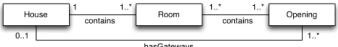
House 1 1..* Room 1..* 1..* Opening
1..* 0..1
contains contains
hasGateways
Figure 1: Domain model of the example Figure 1 gives a very high point of view of a House: it is an aggregation of Rooms, each Room containing at least one Opening. The House itself has at least one opening. In our scenario, these concepts will be kept in the configuration space as classes and each of them supports some variabil-ity represented by a FM. Figure 2 depicts these FMs. The
Housecan have a central computer to manage globally
tem-perature, luminosity and security. Openings can be Doors or Windows, the windows can be a smart tinted glass and have roller stores. We also can put a lock on each opening and a sensor can be put to give the opening state. Each room can have sensors and actuators to manage temperature,
pres-enceor lightning. Moreover the FM expresses some internal
constraints such as “Temperature implies Thermostat”. Constraints between these FMs must also be considered (cf. red arrows in Figure 2). For example, each time a room is configured with a Locking actuator, a Lock on each opening of this local room must also be created. Looking globally at the house, a central security system could oblige, for exam-ple, to have a lock on each opening, to have presence sensors, opened state sensors, roller store actuators and locking ac-tuators.
House Temperature Manager Luminosity Manager Security Manager Opening Sensors Lock Room Sensors Actuators Temperature Lightning Presence RollerStore Thermostat Locking
Temperature implies Thermostat Presence implies Locking
OpenedState Kind Door Window RollerStore TintedGlass Key Mandatory feature Optional feature XOR OR interFM implication CentralComputer
Figure 2: Feature models and excerpt of relations
home:House {House}
entrance:Room {Room}
frontDoor:Opening {Opening, Kind, Door} conf1 home:House {House} entrance:Room {Room,Sensors, Presence,Actuators, Locking} frontDoor:Opening {Opening, Kind, Door, Lock,
Sensors, OpenedState}
mainRoom:Room {Room,Sensors,Lightning}
mainRoomDoor:Opening {Opening, Kind, Door, Lock}
mainRoomWindow:Opening {Opening, Kind, Window,
TintedGlass} conf2
Key
instanceName:Type {configuration features}
Figure 3: Example of two valid configurations of an House instance that conforms to these specifications. Figure 3 gives two examples of such valid configurations. The first configuration, at the top, is a minimal valid config-uration respecting both the domain model and the feature models. The second configuration is a bit more complex, but it also respects all given constraints.
2.3
Overview of the Approach
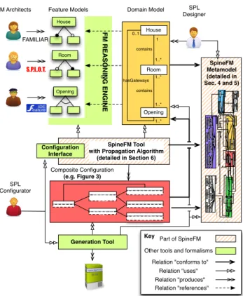
Our approach is summarized on Figure 4. The SpineFM toolchain allows to design SPLs so to create composite con-figurations. In SpineFM, a SPL is defined by (i) a domain model that represents, at the end-user level, the concepts of the software family, their multiplicities, and how these concepts are interrelated; (ii) FMs that capture the com-monalities and variabilities of each concept, also at end-user level; and (iii) constraints between these FMs.
For example, in our running example, the SPL is defined by the domain and FMs respectively depicted in Figure 1 and 2. These concepts are defined in a dedicated metamodel presented in section 3. Our solution supports end-user def-initions of complex configurations, i.e., an instance of the domain model, whose elements refer to FM configurations. The configurations introduced in the previous section and depicted in Figure 3 are representations of our composite configurations for the running example.
The part of the metamodel formalizing composite configu-rations and concepts underlying the derivation process are described in section 4. These composite configurations serve as inputs for a dedicated generation tool that builds concrete products, but in this paper, we only focus on its definition
Opening House
Room
FM Architects Feature Models Domain Model
Configuration Interface SpineFM Metamodel (detailed in Sec. 4 and 5) Generation Tool SPL Designer SPL Configurator
Key Part of SpineFM
Other tools and formalisms Relation "conforms to"
Relation "uses" Relation "produces" F M R EA SO N IN G EN G IN E Relation "references" S.P.L.O.T. FAMILIAR SpineFM Tool with Propagation Algorithm
(detailed in Section 6) Composite Configuration (e.g. Figure 3) House Room Opening 1 1..* 1..* 1..* 1..* 0..1 contains contains hasGateways home:House {House} entrance:Room {Room,Sensors, Presence,Actuators, Locking} frontDoor:Opening {Opening, Kind, Door, Lock,
Sensors, OpenedState} mainRoom:Room
{Room,Sensors,Light ning}
mainRoomDoor:Opening {Opening, Kind, Door, Lock} mainRoomWindow:Opening {Opening, Kind, Window,
TintedGlass} RFMod el RestrictionFunction Ru le Configur ationStat e 1 rules state 1 1..* 0..* selected deselected fm refers_on MSPLMode l Domai nElement DEAssoc iation
DEAssociationEndyElementMultiplicit
s 1..* 0..* 0..* 2 1 1 1 concepts associations belongs_to extremity apply_on conceptMultiplicity linkMultiplicity 1 functions 0..* F MM odel Featu reModel raintConst
children features root constraints 1..* 0..* 0..* 1 Fe ature Group ConfigurationModel CompositeConfiguration Configurat ion Link subConfigurations 0..* source target belongs_to 1 1 0..* state related 1 1 Proc essM odel Glob alContextLocal Context Context Manage r ConfigurationP rocessStep 1..* CPS locals global 1 0..* 1 DE configuration 1 configurations 1..* 1 MPL 1 CPS 0..* links inverse source target UserA ctionModel UserActi on UserS elect User Deselect User Propagate UserV alidC onfiguratio n UserLinkC onfiguratio n User Generat e UserSave Past UserRenameElem ent UserCreateContex t UserCloneContext SystemActionM odel SystemAction Action OnFM ActionS elect ActionD eselect ActionCreate Configuration Acti on Link ActionCr eateCont extActionMoveC onfiguration ActionDelete Context ActionAddCT Constraint ActionAbstra ctRename ActionRenam eCPS ActionRenam eConfig ActionRenam eProduct action 1 contextManager 1 past launchingAction launchedActions 0..* configuration 1 actionsDone 1..* state 1 0..1
Figure 4: Overview of the approach
and the configuration stages. The derivation process is based on a propagation algorithm that continuously ensures the consistency of the partial composite configuration by au-tomatically triggering configuration actions with respect to model instances and previous actions. The algorithm and its properties are described in section 5.
3.
A DOMAIN MODEL WITH
INTERRE-LATED FMS
The domain model and its related FMs serve both to design the SPL and to drive the user through the derivation process. Figure 5 shows an excerpt of the metamodel that defines the concepts supported in a domain model. These concepts are organized in three packages: DomainMetamodel gathers concepts for the domain elements, associations and multi-plicities, FMModel contains all concepts to represent and manipulate FMs, and finally RFModel consists of concepts managing constraints between FMs.
RFModel RestrictionFunction Rule ConfigurationState DomainMetamodel DomainElement DEAssociation DEAssociationEnd MultiplicityElements DomainModel 1..* 0..* 0..* 2 1 1 1 concepts associations belongs_to extremity apply_on conceptMultiplicity linkMultiplicity functions FMModel FeatureModel Constraint children features root constraints 1..* 0..* 0..* 1 Feature Group ActionOnFM Keyexternal package :Concept from an
0..* action 1 refers_on 1 deselected selected 0..* 1..* 1 fm inverse 1 state 1 rules 1..*
Figure 5: Domain model and interrelated FMs
3.1
Concepts, Associations and Multiplicities
In the domain model, concepts are Domain Elements (DE) and associations between them are DEAssociation. Each DE is related to a FM representing its specific variability. Asso-ciations are not oriented and two domain elements are only related by a unique association. This enables to focus on a unique association when relating their FMs. Each DE sup-ports its own multiplicity to allow its multiple instantiation in configurations. Associations extremities (DEAssociatio-nEnd in the metamodel) also express multiplicities to con-trol the number of associated instances of DE. Unbounded multiplicities are supported and bounded multiplicities are limited to 0 or 1. The different restrictions on the domain model enables to simplify the interrelations between FMs, but in our experience, this is expressive enough to capture and represent complex configurations.
Figure 1 shows a domain model using all these concepts: House, Room and Opening are domain elements; the three relations (the two contains and the hasGateways) are DE-Associations; we only represent the multiplicities on associ-ations extremities on this figure.
3.2
Representation of Feature Models
Each domain element is an abstraction of a configuration
space, i.e., a FM capturing some variability. The
pack-age FMModel provides concepts to represent and
manip-ulate such FMs1. A FeatureModel is a set of Features and
Constraints. Each Feature, except the root, is a part of a Group which has an attribute specifying its state between Mandatory, Optional, Or, Alternative-Or and Mutex.
SpineFMsupports different FM formalisms (e.g., SPLOT,
FeatureIDE, TVL and FML) by delegating operations on FMs to an external reasoning engine. For example, the three FMs in Figure 2 could have been represented using
indiffer-ently SPLOT, FeatureIDE and TVL, at the same time2.
From now on, we use the term “sub-configuration” to qual-ify indifferently an instance of a DE or a configuration of a FM: we formalize this notion in section 4.1.1.
3.3
Restriction Functions
Associations between DEs also aims at managing the rela-tions between configuration spaces. As different sub-config-urations are not necessarily compatible, constraints between FMs must be expressed and enforced. For example, in sec-tion 2.2 we expressed that a House with a “SecurityManager” imposes to have a “Lock” and an “OpenedState” sensor for each Opening, as well as a “Presence” sensor and “Locking” actuator for each Room. In SpineFM these relations will be expressed as constraints or rules such as if I select Se-curityManager in House, the feature Lock is automatically selected in my future sub-configuration of Opening.
The package RFModel provides concepts to express such rules. These rules are grouped in a RestrictionFunction that complements DEAssociations. A restriction function is ori-ented from a source FM to a target one, and contains several Rules. A rule is defined as a trigger from an instance of the source and an action to be performed on an instance of the target. The trigger is a ConfigurationState, it represents a
1This FM metamodel is partially extracted from the project
http://www.eclipse.org/featuremodel/ focusing on
ele-ments used by the propagation algorithm.
2However SpineFM is currently limited to propositional
FMs.
specific state of a FM configuration (the sets of selected fea-tures and the set of deselected ones). SpineFM supports different actions on FMs (ActionOnFM concept): select or deselect on a feature, and addConstraint to add a new cross-tree constraint in the FM.
Finally, as associations are not oriented and restriction func-tions are, they must be implemented in both ways of the as-sociations. In order to ease the design of the SPL, the inverse restriction functions and rules are automatically computed and maintained by SpineFM.
4.
DERIVING A COMPOSITE
CONFIGU-RATION
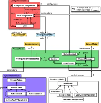
The domain model and related FMs are also used to derive composite configurations in a consistent way. Figure 6 shows an excerpt of the four packages in the SpineFM metamodel that deal with composite configurations: a Configuration-Model represents a composite configuration; ProcessConfiguration-Model captures concepts to derive consistent configurations in a non-ordered process; SystemActionModel and UserAction-Model are used to realize derivation actions on the SPL. To simplify the representation, we do not show on Figure 6 all available actions, neither all references between SystemAc-tions and the different concepts of the metamodel.
ProcessModel Context GlobalContext LocalContext ContextManager ConfigurationProcessStep CPS locals global 1 DomainModel DomainElement 0..* 1 DE 1 1..* DomainModel
Key Concept from an
external package : ConfigurationModel CompositeConfiguration SubConfiguration Link subConfigurations 0..* source target belongs_to 1 1 0..* DEAssocation ConfigurationState state related 1 1 1..* configuration configurations 1 0..* links UserActionModel UserAction UserSelect UserDeselect UserValidConfiguration UserLinkConfiguration SystemActionModel SystemAction ActionOnFM ActionSelect ActionDeselect ActionAddCTConstraint contextmanager 1 actionsDone 1..* state 1
Figure 6: Composite configuration (metamodel ex-cerpt)
4.1
Composite Configurations
The configuration of a SpineFM SPL is defined by a Com-positeConfiguration, which is a composition of linked Sub-Configurations. A SubConfiguration is itself a FM configu-ration related to a domain element instance. The Compos-iteConfiguration contains Links that connect a source sub-configuration to a target one. It is important to note that a Link refers to a related DEAssociation as it can be seen as an instance of this association.
Figure 3 depicts two examples of such composite configu-rations containing respectively 3 and 6 sub-configuconfigu-rations for the different domain elements House, Room and Open-ing. In the first composite configuration, the link between
the sub-configurations “fromDoor” and “home” corresponds to the association “hasGateways” defined in Figure 1 that relates House and Opening.
4.1.1
Properties
A SubConfiguration is a configuration of a FM as defined by Benavides et al. : “Given a FM with a set of features F, a configuration is a 2-tuple of the form (S, R) such that
S, R ⊆ F being S the set of features to be selected and R
the set of features to be removed such that S ∩ R = ∅.” [6]. A configuration is defined as a ConfigurationState in which each feature of the FM belongs either to the set of selected or deselected features w.r.t. to the FM semantics (i.e., cross-tree constraints and feature groups are respected). A com-posite configuration is valid and complete w.r.t. to a do-main model if (i) multiplicities of associations are respected, (ii) multiplicities of concepts are respected, and (iii) sub-configurations are valid and compatible. The composite con-figuration then conforms to the domain model.
Both composite configurations presented in Figure 3 are con-forms to the domain model presented in Figure 1 following this definition. Multiplicities of associations are respected: the House is connected to a unique Opening in both com-posite configurations, each House has at least one Room and each Room one Opening. Assuming we can only in-stantiate a unique House per composite configuration, and as many Rooms and Openings as desired, multiplicities of concepts are respected too. Finally each sub-configuration is valid w.r.t. its FM and linked sub-configurations are compat-ible. For example, the “entrance” sub-configuration (second composite configuration on Figure 3) contains a “Locking” feature, so it is linked to Opening sub-configurations with “Lock” feature as expressed by red arrows in Figure 2.
Moreover we define the consistency of the SPL as the re-alizability of each sub-configurations of the SPL [22]. This means that for all valid sub-configuration of each domain el-ement, it exists a minimal composite configuration conform-ing to the domain model that contains it. In other words, the SPL does not contain any “dead” sub-configurations, by analogy with the dead features definition in feature model-ing.
4.2
Derivation Process
SpineFM must ensure that the derivation of a composite
configuration is an order free process. The user is thus only authorized to do specific actions, which are based on her previously done actions. SpineFM then manages different contexts of configuration, so to support a staged composite configuration process, enabling partial configurations with-out following any predefined configuration workflow. We distinguish two kinds of actions in our system: user ac-tions (package UserActionModel ), and system acac-tions (pack-age SystemActionModel ). User actions provide a high level of abstraction to realize coargrained actions such as se-lecting a feature or linking two sub-configurations. More-over these actions create and orchestrate the system actions, which manipulate the different concepts of the metamodel. Different kinds of system and user actions exist, e.g., , to create a configuration, a link, or rename elements, but we only deal here with actions on FMs, corresponding to selec-tion/deselection of features, and creation of cross-tree con-straints inside FMs.
The different actions realized on FMs can have impacts (i.e.,
se-lection or desese-lection) on the other ones, following the re-striction functions. For example, we explain in Section 2.2 that if a feature “Security Manager” is selected in the House sub-configuration, then some features must be selected in all sub-configurations of Room and Opening. The key idea is that realizing this sub-configuration of the House will glob-ally impact all the other sub-configurations of Room and Opening. We use here the term “global” to insist on the fact that all further sub-configurations will be impacted. On the other hand, if we select in a specific Room sub-configuration a “Locking” actuator, then only the associated (but all of them) Opening sub-configurations should have a “Lock” fea-ture. This means that realizing a sub-configuration of the Room will locally impact the sub-configurations of Open-ing. The term “local” expresses here that impacts are only localized on few sub-configurations.
To manage these impacts and their propagation, we define the notion of Context. A unique Global Context manages all the global impacts and many Local Contexts are used for the local ones. More precisely, information about the impacts are contained in the concept of ConfigurationPro-cessStep (CPS), which represents a FM being configured. A CPS contains (i) a reference to the domain element it rep-resents; (ii) references to the actions done on the FM; and (iii) the current configuration state of the associated FM (see section 3.3).
A context only contains a unique CPS for each DE. More-over, contexts are closely related to the multiplicity of the DEs. If a DE can be instantiated only once (upper multi-plicity is 1) in a composite configuration, then there is no need to keep another CPS for this DE on each context. We only need a unique CPS contained in the global context to represent the state of this DE. However if a DE can be in-stantiated many times, it does not mean its CPS will only exist in a local context. In fact, each context (local and global) of the system will contain a CPS for these DEs. We illustrate the notion of context with the following sce-nario: A user starts the derivation by selecting the feature “Sensors” in a Room. Now if she continues by selecting the feature “SecurityManager” in the DE House, the CPS of House in the global context is impacted, as the House can only be present once in a composite configuration. As some rules are associated to this feature (see red arrows on Figure 2), the CPS of Room in the global context is also impacted to select “Presence”, “RollerStore” and “Locking” once for all: all the further Rooms she could create need to have these features selected. But at this moment, these 3 features are not selected in the CPS of Room in the first local context, and that could lead to inconsistent user ac-tions (e.g., deselecting “RollerStore”). That is why the same impacts are also applied in the CPS of Room in the first lo-cal context, selecting the 3 features ‘Presence”, “RollerStore” and “Locking”.
Consequently the ContextManager can be seen as the wizard of the derivation process. It contains all the contexts of the system and manages the different operations to create new contexts and to propagate actions through them.
5.
PROPAGATION
In order to propagate the actions triggered by restriction functions through the different contexts of the system, SpineFM relies on a propagation algorithm. The propagation is trig-gered from a CPS that belongs to a context. Each time a user does an action like selecting or deselecting a feature, the
propagation is triggered from the impacted CPS. A strong hypothesis to use this propagation algorithm is that the SPL must be consistent (see section 4.1.1).
We thus check the SPL consistency each time a new sub-configuration is added into the SPL. This checking process uses our propagation algorithm to verify the compatibility of a sub-configuration with the others. However we can reduce the complexity of the process by considering the domain model as a graph and restricting propagations to the bi-connected domain elements. Considering the SPL as consis-tent, adding a new sub-configuration only requires to check few connected components to ensure the realizability of the new part.
5.1
Description of the Algorithm
The algorithm is recursive and comprises four main steps: (i) it computes the actions to be triggered in the different CPSs of the same context, following the associations; (ii) it applies the actions on the targeted CPS; (iii) for each impacted CPS that belongs to the global context, it applies the same impacts to all CPS related to the same domain element in local contexts; and finally (iv) it triggers back the propagation from each newly impacted CPS.
We now describe the main functions of the propagation al-gorithm. We consider that the GlobalContext (noted GC) and the set of LocalContexts (noted SetOfLocalContexts) are global variables accessible from everywhere. We also use a dot notation similar to the Java implementation.
Function 1 propagate(cps:CPS, cont:Context):void
1: setOfCPS := restriction(cps, cont) 2: recursePropagation(setOfCPS, cont)
Function 1 is the entry point of the propagation. It takes as inputs a CPS impacted by an action and its related con-text. This function first computes and applies actions on CPSs of the same context. Then the list of resulting im-pacted CPSs is used to trigger the propagation recursively and apply global impacts in local contexts.
Function 2 restriction(cps:CPS, cont:Context):Set
1: result := ∅
2: deSrc := cps.getDE()
3: assoSrc := deSrc.getAssociation() 4: for allasso ∈ assoSrc do
5: deTarget := assoSrc.getOtherEnd(deSrc) 6: multTarget = deTarget.getMultiplicity() 7: ifmultTarget.upperBound() = 1 then 8: cpsTarget := GC.getCPSofDE(deTarget) 9: else 10: cpsTarget := cont.getCPSofDE(deTarget) 11: setOfActionsToDo := getActions(asso, cps) 12: for allaction in setOfActionsToDo do
13: ifcpsTarget.getActionsDone() ∩ action = ∅ then
14: result.add(cpsTarget)
15: action.setCPS(cpsTarget)
16: action.apply()
17: return result
Function 2 computes and applies actions to be triggered on CPSs that belong to the same context as the original ac-tion. It takes as inputs the CPS that is responsible for the propagation and its associated context. To ease reading in the following, we call this context the propagation context. The function iterates on associations to which the DE be-longs (lines 4 to 16). For each association, the target DE is the one referenced by the other association end (line 5).
Then the CPS to target is selected w.r.t. to the multiplic-ity of the target DE (lines 7 to 10): if the DE has a upper multiplicity of 1, then the CPS must be retrieved from the global context, otherwise it is taken from the propagation context. The function retrieves the list of actions to trigger on targeted CPS (line 11, this function is detailed below). Finally it iterates on each action (line 12), verifies that the action has not been yet applied on the targeted CPS (line 13) and if not, it adds the targeted CPS to the resulting list of impacted CPSs (line 14) and applies the action (lines 15-16).
Function 3 getActions(asso:DEAssociation, cps:CPS):Set
1: result := ∅
2: CS := cps.getState()
3: for allrf ∈ asso.getRestrictionFunctions() do 4: for allrule ∈ rf.getRules() do
5: ruleCS = rule.getState()
6: if ruleCS ∩ CS = ruleCS then
7: result.add(rule.getAction())
8: return result
Function 3 compares a list of rules with a configuration state and selects which actions to apply on a CPS. It takes as in-puts an association and the CPS triggering the actions. To compute the actions to apply, the function starts by getting the ConfigurationState (CS) corresponding to the CPS (line 2). Then it iterates on each rule of each restriction func-tions of the association (lines 3-4) and checks whether a CS of a rule matches with the CS returned from the CPS (line 6): a match means that a rule can be fired. The match-ing part consists in computmatch-ing the intersection between two CS, which directly corresponds to the intersection of their respective sets of selected and deselected features.
Function 4 recursePropagation(setOfCPS:Set,
cont:Context):void
1: for allcps ∈ setOfCPS do 2: deTarget := cps.getDE()
3: multTgt := deTarget.getMultiplicity()
4: if (multTgt.upperBound() = 1) or (cont = GC) then
5: propagate(cps, GC)
6: if notmultTgt.upperBound() = 1 then
7: for alllocCtx ∈ SetOfLocalContexts do
8: localCPS := locCtx.mergeWithCPS(cps)
9: propagate(localCPS, locCtx)
10: else
11: propagate(cps, cont)
Function 4 then performs the propagation recursively. It takes as inputs the set of CPS which has been impacted by restrictions (Function 2) and the propagation context. The function iterates on each CPS handling two possibilities. The first one is the case where the CPS refers to a DE with a upper multiplicity higher than 1 and the context given as input is local, then the propagation is triggered with this CPS (line 11). If one of the previous conditions is not met, i.e., the CPS refers to a DE with a upper multiplicity of 1 or the context corresponds to the global context (line 4), the propagation is applied on the global context (line 5). However, if a CPS with a upper multiplicity higher than 1 is impacted in the global context (line 6), then all CPSs referring to the same DE in local contexts must reflect the same impacts (line 7). This is exactly the case at the end of the last example of section 4.2. Actually the function mergeWithCPS, which takes a CPS as input, looks in the context to retrieve a CPS with the same referring DE and apply in this last CPS all actions applied in the CPS given in argument. Finally, as all local contexts can have new impacts, the propagation is also triggered from them.
5.2
Termination of the Algorithm
The propagation algorithm is based on actions triggered by a user action on a CPS. A CPS cannot be modified twice by the same action because of the idempotence of all supported actions. In Function 2 we check if an action has already been done (line 13) to reduce the algorithm complexity and to know exactly which CPSs have been impacted. Moreover, the system actions associated to restriction functions (and triggered by the propagation) are only FM actions to select or deselect features, or to add a constraint.
Consequently the configuration space associated to CPS is always decreasing, each step of the propagation reducing the number of allowed actions. This shows that the algorithm al-ways terminates and a propagation results in the application of all the rules once on each context, in the worst case.
6.
EVALUATION
In this section, we elaborate on the implementation and the evaluation of our approach based on a real-world case study. We evaluate our approach by tracing the derivation pro-cess while creating configurations. We want to verify the relevance of the approach w.r.t. (i) the need for complex configurations (see Section 6.4.1), (ii) the variability of the SPL (see Section 6.4.2), and (iii) impacts of the algorithm on propagation time (see Section 6.4.3) and memory usage (see Section 6.4.4). We also discuss the threats to validity regarding our evaluation.
6.1
Implementation
The solution described in this paper has been entirely im-plemented in Java 6 using the Eclipse Modeling Framework
(EMF) for the metamodeling part3 SpineFMis constituted
by more than 90 KLOC and around half of them are gener-ated using EMF. It can be used through a REST API which allows to create any of the user actions. SpineFM is con-nected to the FAMILIAR DSL, which provides a language and API facilities to manipulate and reason on different fea-ture model formalisms [1].
A generic user interface is also provided to support the derivation process. The interface is not dedicated to a spe-cific domain model but uses meta-data associated to feature models and domain models [30]. The implementation of the interface uses the Javascript framework AngularJS and is around 7 KLOC. Finally a generation tool for YourCast products (YourCast is described more in details in the next section) has also been created using Java 6 and EMF, rep-resenting more than 95 KLOC. The tool relies on different EMF transformations, taking as input the composite config-uration and the domain model, and transforming them to an architectural model of the solution. Then other transforma-tions are applied to create specific component models until a final model-to-code transformation that uses templating facilities from the Velocity engine.
6.2
YourCast
YourCast4is a project initiated in 2011 which aims at
creat-ing an industrial-strength SPL for Digital Signage Systems (DSS) [28]. A DSS broadcasts dynamic information, mainly from the Web, typically targeting both public institutions and private companies. This project involved during two and half years around 30 contributors realizing more than
3More information about SpineFM will be soon available at
http://www.yourcast.fr/en:spinefm.
4http://www.yourcast.fr
470 KLOC for the assets of the SPL and two software archi-tects for the design of the SPL.
Several products have been generated using the complete toolchain mentioned above, including SpineFM as reasoning engine, the user interface to create the configuration and the generation part to create the concrete product. Some of the generated products have been notably deployed on several university campuses, on our laboratory, during conferences, or for big events like the “Choralies” an event which involves more than 4000 of participants in the south of France. We discuss in the following paragraphs the realization of some of these products and use them as starting points to evaluate different aspects of the proposed approach.
6.3
Evaluation Setup
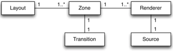
Using SpineFM, a DSS is captured at the domain level by 5 concepts: the Sources of information to display, the Renderer components to display information, the Transition components to move from a piece of information to another, the Zone where to put information on the screen and the Layout to organize the different zones and design the dis-play. Figure 7 gives an overview of the YourCast domain model. We represent inside each domain element box the multiplicity associated to the concept (e.g., a DSS contains one layout and many sources). The domain model also con-tains 2 restriction functions by associations (one for each orientation of the association) and 174 rules, including the automatically computed inverse ones. The rules express con-straints between component like type compatibility between Sources information and rendering components, and style compatibility between zones, renderers, layout, and transi-tions.
Layout Zone Renderer
Source Transition 1 1 1 1 1 1 1..* 1..*
Figure 7: YourCast Domain Model
The table 1 gives some figures about feature models used in the YourCast project. Our feature models have small size in terms of features but are highly constrained, as they are actually automatically built by merging feature models describing individual products by using a logical operator defined in the FAMILIAR tool [2]. This operation allows us to manage the evolution of our feature models, however it imposes to create a lot of constraints inside feature mod-els [27].
Concept # Features # Constraints # Config.
Sources 81 154 68 Renderers 76 347 74 Transitions 33 45 15 Zones 49 160 27 Layouts 51 59 13 Average 58 149 39 Total 290 765
-Table 1: YourCast feature models
Our experimental setup consists in configuring different Your-Cast products to gather different kinds of metrics. All
con-figurations have been realized on a virtual machine exploit-ing a Linux Debian 6.0.8 system with 4096 Mb of RAM and 4 CPUs at 2.4 Ghz. The toolchain was running on a Tomcat 6 application server limited to 512 Mb of memory. The Java version used was 1.6.0 build 26.
The configurations have all been realized by two different users through our configuration interface. Both users were already familiar with the DSS domain and with the config-uration interface.
6.4
Result Analysis
6.4.1
Realized configurations
We show in table 2 the metrics gathered after the derivation process of 5 deployed YourCast products (named A to E). They cover different product sizes, that one can estimate by adding numbers of sub-configurations and links. It is in-teresting to note that no particular workflow has been used to built these products: e.g., some products have been cre-ated starting by the layout, other by sources, showing the order-free capability of the configuration process.
A B C D E Avg. sub-config. 37 9 25 23 61 31 links 36 8 24 22 60 30 contexts 19 5 13 12 32 16.2 CPS 77 21 53 49 129 65.8 User act. 259 68 194 172 348 208.2 Sys. act. 4111 849 2835 2703 7218 3543.2 Auto. act. 631 140 462 399 1492 624.8 FM actions 3480 709 2373 2304 5726 2918.4 % user act. 5.93 7.42 6.40 5.98 4.60 5.55 % sys. act. 94.07 92.58 93.60 94.02 95.40 94.45
Table 2: Metrics on YourCast Configurations This gives some first insights on the configuration process. First, the number of sub-configurations and links seems to be always related, which is consistent as the composite configu-rations conforms to the domain model described in Figure 7. The number of contexts is also directly proportional to the number of configurations being built by the user.
The theoretical number of contexts is indeed bounded by the number of configurations: it corresponds to at least one context (the global one) and at most twice the number of configurations being built by the user, these extra contexts handling unbounded multiplicities (i.e., 1..*). We can notice that the average number of contexts is significantly lower than the upper bound of this theoretical number.
As for actions, we split the measure into four categories: we distinguish user actions and system actions as explained in 4.2. Then system actions are divided into two categories: the automatic actions, triggered by restriction functions, and the FM actions. These are implicit actions realized by FAMILIAR back-end solvers (SAT or BDD depending on the operations), when configuring the FM, so that it re-mains valid, e.g., selecting automatically a parent feature or applying a constraint. We observe that the number of user actions is very low in comparison with the total number of system actions, emphasizing the need for an automatic derivation process to create complex products. Moreover as the system actions are only feature model actions, it gives an interesting insight on the size a unique feature model would have to capture equivalent configurations (e.g., more than 4000 feature in case A). Finally we also observe that feature model actions are far more frequent than automatic actions.
Though our figures obviously depend on the design of our feature models, this shows that our approach can support a configuration process with automatic propagation while relying on feature models and usual solvers.
6.4.2
Number of configurations
As the variability captured in an SPL is related to the num-ber of configurations it represents, we determine how to com-pute a potential number of composite configurations given the domain model and the number of feature model config-urations.
In YourCast, let CL, CZ, CR, CS and CT be the respective
number of configurations for Layout, Zone, Renderer, Source, and Transition elements (all figures are available in Table 1). We define Z as the total number of zones in a composite con-figuration, as a layout can be associated with many zones, and we define R as the total number of renderers associated to a zone (assuming that each zone has the same number of renderers), as a zone can have many renderers. Then we can compute N , the number of potential composite config-urations depending on Z and R, following this formula:
N = CZ! (CZ−Z)!× CR! (CR−(R×Z))!× CS! (CS−(R×Z))!× CT! (CT−Z)!× CL
However N is an upper bound of configurations, as it does not take into account the compatibility and restriction be-tween products.
The average number of zones in the considered products is around 3 and the average number of renderers per zone is around 4. Then given Z = 3 and R = 4, we obtain N =
2.28 × 1052potential complex configurations. Even if Z = 1
and R = 1, this leads to a composite configuration with only one instance of each concept, the number of available configurations being N = 26.493.480. The very high number of possible combinations emphasizes the high variability and the great complexity of the SPLs one can manage with the proposed approach.
6.4.3
Propagation time
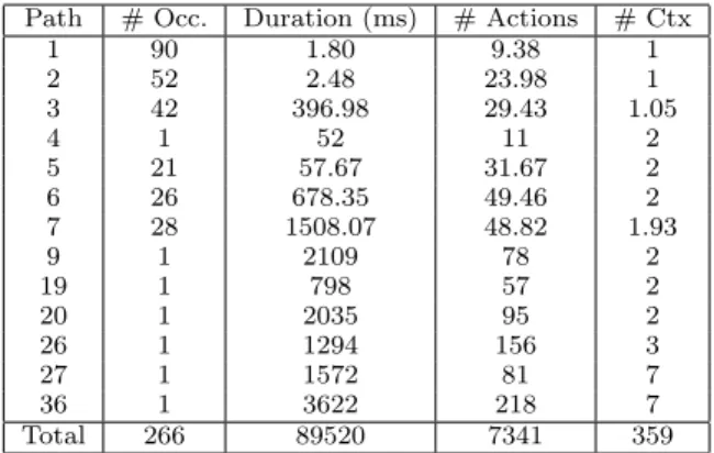
In our approach the propagation algorithm is key to the configuration process. Therefore it is essential that prop-agation time remains short enough to keep the user focus on her configuration task. During the 5 configurations de-scribed in Table 2, 266 propagations occured (propagations are part of user actions). We also gathered metrics on them, presented in Table 3, classifying them by the length of the propagation path. We define a propagation path as the num-ber of CPS impacted during the propagation. The second column gives the number of occurrences of propagation of a given path length. The three last columns give respectively the average duration of the propagation in milliseconds, the average number of system actions and the average number of impacted contexts. The last line shows the total number of propagation occurences, duration time, number of system actions and number of impacted contexts.
First we can notice that the 266 propagations on the 5 con-figurations involved more than 7000 system actions. A high percentage of these propagations only impact a single con-text, making the propagation very fast. It is interesting to note that propagations with a path length greater than 7 are very rare (only one occurence of each). Actually this number of 7 seems to be strongly related to the considered domain model. In our YourCast model, a propagation may impact 4 concepts simultaneously in the same context, but
Path # Occ. Duration (ms) # Actions # Ctx 1 90 1.80 9.38 1 2 52 2.48 23.98 1 3 42 396.98 29.43 1.05 4 1 52 11 2 5 21 57.67 31.67 2 6 26 678.35 49.46 2 7 28 1508.07 48.82 1.93 9 1 2109 78 2 19 1 798 57 2 20 1 2035 95 2 26 1 1294 156 3 27 1 1572 81 7 36 1 3622 218 7 Total 266 89520 7341 359
Table 3: Propagation metrics by number of steps
if the Layout is involved, the global context impacts is then replicated in few local contexts. We think it might also be related to the usual habit to finish a sub-configuration be-fore shifting to another: finished configurations cannot be impacted anymore, which limits the impacted contexts. We also observe that, as expected, in average the longer is the path, the longer is the duration and the more there are system actions. The high duration number obtained for a path length of 3 is not absolutely clear for us, but it can partially be explained by the fact that most propagations of this length have been obtained during the last configuration (configuration E in Table 2), which involved a lot of artifacts. This has obliged the FAMILIAR reasoning engine to use the garbage collector, slowing down the whole execution. Finally we observe that the average number of impacted contexts is very low. Most of the impacts are very local, thus showing the good scalability of the propagation algorithm.
6.4.4
Memory usage
The propagation algorithm relies on the contexts, which are composite entities. Each new context contains as many CPS as concepts in the domain model. Each CPS is associated with a FM configuration through the FAMILIAR DSL. Thus we measured the memory footprint of SpineFM when aug-menting artificially the number of contexts.
We show in Table 4 the result of the memory usage obtained with the bash command free -m.
# Contexts Used memory (Mb) Free memory (Mb)
0 715 3301 1 878 3138 10 879 3136 50 879 3136 100 883 3132 500 933 3082 750 977 3038 850 1015 3001 1000 1050 2965
Table 4: SpineFM memory evolution by contexts The first measure is taken after the Tomcat server launch, all services being ready: the reported memory usage is the footprint memory usage of the machine. For the second measure, we initialized SpineFM with YourCast informa-tion: the global context is automatically created. Then all other measures are taken after having activated some Cre-ateContext user actions through the SpineFM API. Table 4 shows that from 1 to 1000 contexts, the consumed memory
increases gradually, a thousand of contexts taking around 170 Mb of memory. This experiment points out that our tool easily supports configurations with thousands of sub-configurations for a SPL of the size of YourCast.
However we can also notice that the initialization of a first configuration of YourCast took 163 Mb of memory, which is significant. This amount of memory can be explained by the usage of FAMILIAR to manage our FMs: the first initialization of SpineFM with a domain model imposes to load the associated FMs in FAMILIAR, which is memory consuming. Moreover, in YourCast, FMs are defined as the result of a merging operation in FAMILIAR, which is also known to be memory consuming [2].
To emphasize the memory consumption related to SPL con-figurations (and not only due to context management), we measured the memory consumption during the realization of the 5 products given in Table 2. The measures, also ob-tained with the command free -m, are shown on Table 5. Here the memory consumption for the first configuration
# Config Used memory (Mb) Free memory (Mb)
0 736 3280 1 913 3102 2 922 3094 3 938 3078 4 947 3069 5 963 3053
Table 5: SpineFM memory evolution by config. was around 175 Mb of memory: it corresponds to the first initialization of the system, as explained above. Afterwards, each configuration took less than 20 Mb of memory, which seems reasonable.
6.5
Threats to Validity
A first internal threat to validity concerns the termination of our algorithms. Even if we demonstrated in section 5.2 that our propagation algorithm terminates, bugs in the im-plementation could occur. The SpineFM implemented is thus completed by unit tests and some coverage of differ-ent scenarii in order to minimize such a risk. Moreover we are currently formalizing the whole approach, which will al-low us to formally verify our set of algorithms. Another internal threat concerns our memory measures. Actually as SpineFM embeds the FAMILIAR toolkit, it is hard to distinguish what is really used by SpineFM or by FAMIL-IAR. A more complete evaluation based on the number of instantiated objects in SpineFM during a high number of configurations should give us more confidence in the first results presented here.
The main external threat to validity is related to the low number of experiments we currently conducted. We only applied our approach in one real case study with the Your-Cast project. Nevertheless the approach shows its usability during the project, and experiments on another real case study have already been scheduled to complement our re-sults [29].
Another external threat to validity concerns the users in-volved in our evaluation as they already knew the YourCast system and the configuration interface. However we esti-mate that the obtained metrics are not strongly related to the user behaviors. Moreover we are actually conducting user experiments with ergonomists to evaluate the
config-uration process on the SpineFM user interface supporting undo actions. This should help us to improve both the con-figuration process and the interfaces for further evaluations.
7.
CONCLUSION
In this paper, we described SpineFM, a tooled approach that allows to handle complex configurations in SPL. The SPL is then organized around a domain model and interrelated fea-ture models. The approach enables users to create complex configurations in an order-free process, while being guided thanks to a consistent propagation of actions. We also re-ported on the application of the approach on the develop-ment of industrial-strength family of digital signage systems, showing its good performance on a medium-scale SPL. At short term we are going to apply our approach to an-other real SPL of cyber-physical systems, aiming to refine and validate our proposals. A formalization of the whole set of algorithms will complement this validation. As future work, we plan to extend the SpineFM variability model to support attributed feature models and decision models, and to study more thoroughly the expressiveness of domain mod-els w.r.t. UML model, so to extend its capabilities. As the order free configuration process is at the heart of our so-lution, we also plan to implement our algorithms inside a collaborative configuration environment.
Acknowledgments
The work reported in this paper is partly funded by the ANR YourCast project under contract ANR-2011-EMMA-013-01.
8.
REFERENCES
[1] M. Acher, P. Collet, P. Lahire, and R. France. Familiar: A domain-specific language for large scale management of feature models. Science of Computer Programming (SCP) Special issue on programming languages, page 22, 2013. [2] M. Acher, P. Collet, P. Lahire, and R. B. France.
Separation of Concerns in Feature Modeling: Support and Applications. In AOSD ’12, pages 1–12, 2012.
[3] M. Acher, P. Collet, P. Lahire, A. Gaignard, R. France, and J. Montagnat. Composing multiple variability artifacts to assemble coherent workflows. Software Quality Journal, page 40, 2011.
[4] S. Apel and C. K¨astner. An overview of feature-oriented
software development. Journal of Object Technology (JOT), 8(5):49–84, July/August 2009.
[5] K. B
֒
ak, K. Czarnecki, and A. W
֒
asowski. Feature and meta-models in clafer: mixed, specialized, and coupled. In Software Language Engineering, pages 102–122. Springer, 2011.
[6] D. Benavides, S. Segura, and A. Ruiz-Cort´es. Automated
analysis of feature models 20 years later: A literature review. Information Systems, 35(6):615–636, 2010. [7] J. Bosch. From software product lines to software
ecosystems. Proceedings of the 13th International Software Product Line Conference, pages 111–119, 2009.
[8] J. Bosch and P. Bosch-Sijtsema. From integration to composition: On the impact of software product lines, global development and ecosystems. Journal of Systems and Software, 83(1):67–76, 2010.
[9] G. Botterweck. Variability and evolution in systems of systems. EPTCS, 133:8–23.
[10] P. Clements and L. M. Northrop. Software Product Lines : Practices and Patterns. Addison-Wesley Professional, 2001. [11] K. Czarnecki, S. Helsen, and U. Eisenecker. Staged
configuration through specialization and multilevel configuration of feature models. Software Process: Improvement and Practice, 10(2):143–169, 2005. [12] K. Czarnecki and A. W
֒
asowski. Feature diagrams and logics: There and back again. In 11th International
Software Product Line Conference (SPLC’07), pages 23–34. IEEE, 2007.
[13] D. Dhungana, P. Gr¨unbacher, R. Rabiser, and
T. Neumayer. Structuring the modeling space and supporting evolution in software product line engineering. Journal of Systems and Software, 83(7):1108–1122, 2010.
[14] D. Dhungana, R. Rabiser, P. Gr¨unbacher, D. Seichter,
G. Botterweck, D. Benavides, and J. A. Galindo. Configuration of multi product lines by bridging
heterogeneous variability modeling approaches. In Software Product Lines Conference (SPLC), 2011.
[15] H. Hartmann and T. Trew. Using feature diagrams with context variability to model multiple product lines for software supply chains. In SPLC’08, pages 12–21. IEEE, 2008.
[16] H. Hartmann, T. Trew, and A. Matsinger. Supplier independent feature modelling. In SPLC’09, pages 191–200. IEEE, 2009.
[17] G. Holl, P. Gr¨unbacher, and R. Rabiser. A systematic
review and an expert survey on capabilities supporting multi product lines. Information and Software Technology, 54(8):828–852, 2012.
[18] A. Hubaux, P. Heymans, P.-Y. Schobbens, D. Deridder, and E. K. Abbasi. Supporting multiple perspectives in feature-based configuration. Software and System Modeling, 12(3):641–663, 2013.
[19] K. Kang, S. Kim, J. Lee, K. Kim, E. Shin, and M. Huh. Form: A feature-oriented reuse method with
domain-specific reference architectures. Annals of Software Engineering, 5(1):143–168, 1998.
[20] K. C. Kang, S. G. Cohen, J. A. Hess, W. E. Novak, and A. S. Peterson. Feature-oriented domain analysis (foda) feasibility study. Technical report, DTIC Document, 1990. [21] I. d. C. Machado, A. R. Santos, Y. a. C. Cavalcanti, E. G. Trzan, M. M. a. de Souza, and E. S. de Almeida. Low-level variability support for web-based software product lines. In VaMoS’2014, pages 15:1–15:8, New York, NY, USA, 2013. ACM.
[22] A. Metzger, K. Pohl, P. Heymans, P.-Y. Schobbens, and G. Saval. Disambiguating the documentation of variability in software product lines: A separation of concerns, formalization and automated analysis. In RE’07, pages 243–253, 2007.
[23] K. Pohl, G. B¨ockle, and F. J. van der Linden. Software
Product Line Engineering: Foundations, Principles and Techniques. Springer-Verlag, 2005.
[24] M.-O. Reiser and M. Weber. Multi-level feature trees: A pragmatic approach to managing highly complex product families. Requir. Eng., 12(2):57–75, 2007.
[25] M. Rosenm¨uller and N. Siegmund. Automating the
configuration of multi software product lines. In VaMoS, pages 123–130, 2010.
[26] P.-Y. Schobbens, P. Heymans, J.-C. Trigaux, and Y. Bontemps. Generic semantics of feature diagrams. Computer Networks, 51(2):456–479, 2007.
[27] S. Urli, M. Blay-Fornarino, P. Collet, and S. Mosser. Using composite feature models to support agile software product line evolution. In 6th International Workshop on Models and Evolution, pages 21–26. ACM, 2012.
[28] S. Urli, M. Blay-Fornarino, P. Collet, S. Mosser, and M. Riveill. Managing a Software Ecosystem Using a Multiple Software Product Line: a Case Study on Digital Signage Systems. In Euromicro Conference series on Software Engineering and Advanced
Applications(SEAA’14), special issue: Software Product Lines and Software Ecosystems, , pages 1–8, Verona, Italy, Aug. 2014. Elsevier.
[29] S. Urli, S. Mosser, M. Blay-Fornarino, and P. Collet. How to exploit domain knowledge in multiple software product lines? In 4th Int. Workshop PLEASE’2013, pages 13–16. IEEE, 2013.
[30] S. Urli, G. Perez, H. Zitoun, M. Blay-Fornarino, P. Collet, and P. Renevier. Towards Flexible Configuration User Interfaces (in french) / Vers des interfaces graphiques
flexibles de configurations. In Journ´ee Lignes de