HAL Id: hal-00674251
https://hal.inria.fr/hal-00674251
Submitted on 20 Mar 2012
HAL is a multi-disciplinary open access
archive for the deposit and dissemination of
sci-entific research documents, whether they are
pub-lished or not. The documents may come from
teaching and research institutions in France or
abroad, or from public or private research centers.
L’archive ouverte pluridisciplinaire HAL, est
destinée au dépôt et à la diffusion de documents
scientifiques de niveau recherche, publiés ou non,
émanant des établissements d’enseignement et de
recherche français ou étrangers, des laboratoires
publics ou privés.
Application to Point Multiplication
Fabien Herbaut, Pierre-Yvan Liardet, Nicolas Méloni, Yannick Teglia, Pascal
Véron
To cite this version:
Fabien Herbaut, Pierre-Yvan Liardet, Nicolas Méloni, Yannick Teglia, Pascal Véron. Random
Eu-clidean Addition Chain Generation and Its Application to Point Multiplication. INDOCRYPT 2010,
Dec 2010, Hyderabad, India. pp.238-261, �10.1007/978-3-642-17401-8_18�. �hal-00674251�
Random Euclidean Addition Chain Generation
and Its Application to Point Multiplication
Fabien Herbaut1, Pierre-Yvan Liardet2, Nicolas M´eloni3,
Yannick T´eglia2, and Pascal V´eron3
1 Universit´e du Sud Toulon-Var, IMATH, France
IUFM de Nice, Universit´e de Nice [email protected]
2 ST Microelectronics, Rousset, France
[email protected], [email protected]
3 Universit´e du Sud Toulon-Var, IMATH, France
[email protected] ,[email protected]
Abstract. Efficiency and security are the two main objectives of every elliptic curve scalar multiplication implementations. Many schemes have been proposed in order to speed up or secure its computation, usually thanks to efficient scalar representation [30,10,24], faster point operation formulae [8,25,13] or new curve shapes [2]. As an alternative to those general methods, authors have suggested to use scalar belonging to some subset with good computational properties [15,14,36,41,42], leading to faster but usually cryptographically weaker systems. In this paper, we use a similar approach. We propose to modify the key generation pro-cess using a small Euclidean addition chain c instead of a scalar k. This allows us to use a previous scheme, secure against side channel attacks, but whose efficiency relies on the computation of small chains computing the scalar. We propose two different ways to generate short Euclidean addition chains and give a first theoretical analysis of the size and dis-tribution of the obtained keys. We also propose a new scheme in the context of fixed base point scalar multiplication.
Keywords: point multiplication, exponentiation, addition chain, SPA, elliptic curves.
1
Introduction
After twenty five years of existence, elliptic curve cryptography (ECC) is now one of the major public-key cryptographic primitives. Its main advantages, compared to it main competitor RSA, are its shorter keys and the lack of fast theoretical attacks. The recent factorization of an RSA modulus of 768 bits [17] is here to highlight the significant role that ECC will play during the next decade. In particular, it has been shown that ECC is suitable for cryptographic applications on devices with small resources. However, if 160-bit ECC is believed to remain secure, from a theoretical point of view, at least until 2020 [3], physical attacks on cryptographic devices have proved to be an immediate threat [22]. Thus,
G. Gong and K.C. Gupta (Eds.): INDOCRYPT 2010, LNCS 6498, pp. 238–261, 2010. c
software or hardware ECC implementations have to deal with two apparently opposite requirements: efficiency and security. Indeed, protecting a device from physical attacks usually involves costly countermeasures.
In 2007, M´eloni proposed a secure algorithm based on Euclidean addition chains [27]. As they only involve additions, they are naturally resistant to SCA. However, the efficiency of such a method relies on the existence of a small chain computing the scalar. It has been pointed out that finding such a chain becomes more and more difficult when the scalar grows in size. For cryptographic sizes, finding a good chain is costlier than the scalar multiplication itself. So, instead of proposing a new scalar multiplication scheme, we propose to modify the key generation pro-cess. More precisely, we show that it is possible to generate the key as a small Euclidean addition chain, allowing us to use M´eloni’s fast and secure scheme.
From a general point of view, generating keys in a specific shape is not a new idea. Various methods have been proposed through the years to generate scalars belonging to some subset of the set of all possible keys, with good com-putational properties [14,36,41,42]. However, this usually implies some serious security issues [33,34,9,38]. Some methods remain cryptographically secure in the context of a fixed base point but require large amount of stored data [4,15] (Coron et al. [15] suggest to store from 50 to 100 points for the same security level as that considered in the present work). Finally, some schemes use special endomorphisms, such as the Frobenius map, on Koblitz curves [20].
From that perspective, our approach is quite different. M´eloni’s scheme only effi-ciently applies on curve in Weierstrass form. Moreover, it is particularly suitable to small devices with low computational resources because of its low memory require-ment (at most two stored points) and resistance to side channel attacks. Yet, gen-erating random Euclidean addition chains leads to several problems. First, what is the size of the keys we can generate for a given chain length? In other words, is it possible to achieve a certain level of security with relatively small chains? The sec-ond problem is that of distribution. Indeed, many different chains of same length can compute the same integer. It is then important to ensure that generating keys this way does not weaken the discrete logarithm problem.
In this paper, we produce the first practical and theoretical results on random Euclidean addition chain generation. We also show that it can lead to efficient and SPA-secure scalar multiplication methods.
This work is organized as follows. In Section 2 we review M´eloni’s scheme. In Section 3 we recall some background about Euclidean addition chains and set notations. In Section 4 and 5, we describe two different families of Euclidean addition chains and give some results on their distribution (notice that in Section 4 two variants are described). Finally, in Section 6 we propose some comparisons with existing side-channel resistant scalar multiplication methods.
2
Scalar Multiplication Using Euclidean Addition Chains
For the sake of concision, we do not give details about scalar multiplication and side channel attacks. We invite the reader to refer to [7,12] for detailed overview of elliptic curve based cryptography.
This section is dedicated to a specific scalar multiplication algorithm based on Euclidean addition chains.
2.1 Euclidean Addition Chains
Definition 1. An Euclidean addition chain (EAC) of length s is a sequence (ci)i=1...swith ci∈ {0, 1}. The integer k computed from this sequence is obtained
from the sequence (vi, ui)i=0..s such that v0 = 1, u0 = 2 and ∀i ! 1, (vi, ui) =
(vi−1, vi−1+ui−1) if ci= 1 (small step), or (vi, ui) = (ui−1, vi−1+ui−1) if ci= 0
(big step). The integer k associated to the sequence (ci)i=1...s is vs+ us, we will
denote it by χ(c).
Example : From the EAC (10110) one can compute the integer 23 as follows : (1, 2) → (1, 3) → (3, 4) → (3, 7) → (3, 10) → (10, 13) → 23 = χ(10110).
2.2 Point Multiplication Using EAC
From any EAC c and any point P of an elliptic curve, it is shown in [27] that a new point Q can be computed using the following algorithm :
Algorithm 1. EAC Point Mul(c:EAC, P:point) Require: P , [2]P Ensure: Q = χ(c)P 1: (U1, U2)← (P, [2]P ) 2: for i = 1 . . . length(c) do 3: if ci= 0 then 4: (U1, U2)← (U2, U1+ U2) 5: else 6: (U1, U2)← (U1, U1+ U2) 7: end if 8: end for 9: return Q = U1+ U2
Algorithm 2. Point multiplication Require: P and an integer k
Ensure: Q = kP 1: c← Find EAC(k)
2: return Q = EAC Point Mul(c,P)
In [27], it is shown that any scalar multiplication can be performed using the preceding algorithm. It is achieved by finding an Euclidean addition chain computing the scalar. We will denote by Find_EAC , the algorithm which returns an addition chain for an integer k.
It has been shown in [27] that the for loop of algorithm 1 can be efficiently implemented on elliptic curves in Weierstrass form using Jacobian coordinates. This leads to a fast point multiplication method resistant to side channel attacks since at each step of the for loop, the same operation is used .
The efficiency of algorithm 2 directly depends on the length of the chains and the complexity of the algorithm Find_EAC. Although finding an Euclidean addition chain computing a given integer k is quite simple (it suffices to choose an
integer g co-prime with k and apply the subtractive form of Euclid’s algorithm) finding a short chain remains a hard problem. As an example, the average length of the computed chain for k with g uniformly distributed in the range [1, k] is O(ln2k) [18]. For 160-bit scalars, experiments have shown that, on average, it is required to try more that 45,000 different g to find a relatively small chain using the Montgomery heuristic [32].
2.3 Our Approach
We propose in this paper to proceed differently. Instead of randomly choosing an integer k and then trying to find a suitable EAC c to finally compute the point kP , we propose to randomly generate a small length EAC c and then compute the associated point on the curve. More precisely, we will see in the next sections that the chains will be chosen in a subset of short chains for key distribution matters.
From definition 2.1, notice the random generation of a s-length EAC boils down to the random generation of a s-bit integer. As an example, algorithm 3 shows how to process Diffie-Helmann key exchange protocol with EAC.
Algorithm 3. Diffie-Helmann using EAC Require: a point P
Ensure: Output a common key K 1: A randomly generates a short EAC c1
2: B randomly generates a short EAC c2
3: A computes Q1=EAC Point Mul(c1, P ) and send it to B
4: B computes Q2=EAC Point Mul(c2, P ) and send it to A
5: A computes K =EAC Point Mul(c1, Q2)
6: B computes K =EAC Point Mul(c2, Q1)
Using this approach we compute points kP for a subset S of all possible values for the integers k. Hence we do not deal any more with the classical Discrete Logarithm Problem but with the Constrained Discrete Logarithm Problem.
Name : CDLP
Input : p a prime number, g a generator of a group G, S⊂ Zp, and gxfor x∈ S.
Problem : Compute x.
The complexity of the discrete logarithm problem (DLP) over a generic group directly depends on the size of this group. It has been shown that the constrained version of this problem (CDLP), where only a subset S of the group is considered, has a similar complexity. Indeed, for a random set S, Ω(!|S|) group operations [28] are required to solve the CDLP. As an example, if one naively chooses to generate random Euclidean chain of length 160 (which means there are 2160of
them), we will see, in section 3, that the biggest integer that can be generated is F164$ 2112.7. This means that the number of elements of the set S is at most
In this paper, we propose to study two families of EAC providing good balance between security and efficiency. In practice, it implies that the chains are long enough so that the corresponding set S of generated keys is sufficiently large, but short enough so that the scalar multiplication remains fast.
3
Notations and Properties
We give in this section some notations and important results for the sequel of this paper.
Definition 2. Let n and p be two integers, we define :
. M as the set of EAC and Mn as the set of EAC of length n > 0,
. Mn,p as the set of EAC of length n > 0 and Hamming weight p > 0.
. χ the map from M to N, such that for m ∈ M, χ(m) be the integer computed from the EAC m,
. ψ the map from M to N × N, such that for m ∈ M, ψ(m) = (vs, us) if
m∈ Ms, . S0 the matrix " 0 1 1 1 #
corresponding to a big step iteration, . S1 the matrix
" 1 1 0 1 #
corresponding to a small step iteration. With these notations, for m = (m1, . . . , ms) ∈ Ms, we have :
ψ(m) = (1, 2) s $ i=1 Smi and χ(m) = &(1, 2) s $ i=1 Smi,(1, 1)'.
Let r and s be two integers, we will denote by mm#the element of M
r+sobtained
from the concatenation of m ∈ Mr and m# ∈ Ms. This way, for n > 0, mn is a
word of Mnr if m ∈ Mr.
For convenience, M0 will correspond to the set with one element e which is
the identity element for the concatenation. For m and m# two elements of M
r such that ψ(m) = (v, u) and ψ(m#) =
(v#, u#) we will say that ψ(m)" ψ(m#) if v" v# and u" u#.
Proposition 1. Let n > 0, Fi be the ith Fibonacci number, αn = (1+√2)n+(1 −√2)n 2 and βn= (1+√2)n −(1−√2)n 2√2 : . ψ(0n) = (F n+2, Fn+3), ψ(1n) = (1, n + 2), χ(0n) = Fn+4, χ(1n) = n + 3, . ∀m ∈ Mn, χ(1n)" χ(m) " χ(0n), and ψ(1n)" ψ(m) " ψ(0n), . Sn 0 = " Fn−1 Fn Fn Fn+1 # , Sn 1 = " 1 n 0 1 # , . (S0S1)n= " αn− βn βn βn αn+ βn # , (S1S0)n= " αn2βn βn αn # .
Proof. The first property is straightforward. The other ones can be proved by induction.
Notice that from Sm+n
0 = S0mS0n, we can recover a well known identity on
Fibonacci sequence, namely :
Fm+n= Fm−1Fn+ FmFn+1. (1)
Proposition 2. Let n > 0 and m = (m1, . . . , mn) ∈ Mn, then the map ψ is
injective and χ(m1, . . . , mn) = χ(mn, . . . , m1).
Proof. We refer to [19] for standard link between EAC, Euclidean algorithm and continued fractions, which explains the second point. It is also explained that if ψ(m) = (v, u) then (u, v) = 1 and the only chain which leads to (v, u) is obtained using the additive version of Euclidean algorithm.
4
A First Family of EAC
We will consider in this section M0
nthe subset of M2nwhose elements are EAC
beginning with n zeros.
4.1 Some Properties of M0 n
From proposition 2 the restriction of χ to Mn is not injective because of the
mirror symmetry property.
Proposition 3. The restriction of χ to M0
n is injective.
Proof. Let x and y be two words of M0
n such that χ(x) = χ(y), and m0n,
m#0n, be the words obtained when reading x and y from right to left. Using
the symmetry property, we have χ(m0n) = χ(m#0n). Let (v, u) = ψ(m) and
(v#, u#) = ψ(m#), then
χ(m0n) = χ(m#0n)
⇔ Fnu + Fn−1v + Fn+1u + Fnv = Fnu#+ Fn−1v#+ Fn+1u#+ Fnv#
⇔ Fn+2(u − u#) = Fn+1(v#− v)
Since (Fn+1, Fn+2) = 1, then Fn+2 divides v#− v. Now from proposition 1,
since v and v# are less or equal than F
n+2 and nonzero, then |v# − v| < Fn+2
which implies that v = v# and so u = u#. Hence ψ(m) = ψ(m#), so m = m#.
Proposition 4. χ(M0
n) ⊂ [(n + 1)Fn+2+ Fn+3, F2n+4], the lower (resp. the
upper) bound being reached by 0n1n (resp. 02n). The mean value is (3 2)
n
Fn+4.
Proof. Let 0nx1y and 0nx0y be two elements of
M0
n where x and y are chains
of size a and n − 1 − a with a ∈ [0, n − 1]. From the definition of χ it follows that χ(0nx1y) < χ(0nx0y). Hence the smallest integer is computed from the
word 0n1n and the greatest from 0n0n. Now χ(0n1n) = &(1, 2)Sn
0S1n,(1, 1)' and
χ(02n) = &(1, 2)S2n
0 ,(1, 1)'. From proposition 1, we deduce that χ(0n1n) = (n +
To compute the mean value, let us consider n independent Bernoulli random variables C1, . . . , Cn such that ∀i ∈ [1, n], Pr(Ci = 0) = Pr(C1= 1) = 1/2. The
mean value is E(X) where X = χ(0nC
1. . . Cn). Now X =&(1, 2)Sn 0 n $ i=1 % Ci 1 1−Ci1 & ,(1, 1)'.
Notice that X is a polynomial of Z[C1, . . . , Cn]/(C12− C1, . . . , Cn2− Cn). As the
Ci are independent then ∀J ⊂ [1, n], E('j∈JCj) = 'j∈JE(Cj), hence
E(X) =&(1, 2)Sn 0 'n i=1 % E(Ci) 1 1−E(Ci) 1 & ,(1, 1)' = &(1, 2)Sn 0 'n i=1 %1 2 1 1 2 1 & ,(1, 1)'. The final result comes from proposition 1 and the equality :
∀n ∈ N∗, "1 2 1 1 2 1 #n = (3/2)n−1 "1 2 1 1 2 1 # .
4.2 Application to Existing Standards Using the set χ(M0
n), we can generate (with algorithm 1) 2n distinct points
χ(c)P for a point P whose order is greater than F2n+4. Of course, when the
order d of the point P is known, we have to choose the largest integer n such that F2n+4< d.
Because of the results on the difficulty to solve the CDLP problem, we have to consider the set M0
n only for n ! 160. For n = 160, we have χ(M0160) ⊂
[161F162+ F163, F324], that is to say
χ(M0
160) ⊂ [2118.6, 2223.6].
Such data fit well with the secp224k1 and secp224r1 parameters where the order of the point P is about 2223.99 [6]. Those parameters are consistent with
ANSI X.962, IEEE P1363 and IPSec standards and are recommended for ANSI X9.63 and NIST standards.
4.3 A Variant for the secp160k1 and secp160r1 Recommended Parameters
In the secp160k1 and secp160r1 recommended parameters, the order d of the point P is around 2160. Using the set M0
n, this leads us to choose n = 114
which only gives rise to 2114 distinct points. Hence the complexity of an attack
is Ω(257) which may expose this method to some attacks.
Notice that if we use an element c of M0
160with the point P of order d then
the algorithm 1 computes (χ(c) mod d)P . If the values of {χ(c) mod d, c ∈ M0
160} are well distributed among Z/dZ, then we can use the above mentioned
method, provided that computing χ(c)P with algorithm 1 be more efficient than computing kP with k ∈ Z/dZ, with a classical SPA-resistant method. This last point will be discussed in section 6, we will focus now on the problem of the distribution. To this end, we will adapt results on Stern sequences from [35].
Table 1. Distribution of χ(M0 n) modulo d !n!t 0 1 2 3 4 5 6 7 8 9 10 11 12 13#χ(Mn0 ) d 10 294 312 214 70 12 4 1 0.66 15 10814 12044 6216 2026 436 76 15 0.66 20 266749 327372 194442 74219 20589 4344 789 100 18 1 0.7 25 6493638 8894037 5979946 2627531 850691 216285 44567 7832 1233 162 15 1 1 0.74 29 74024780 115132679 88980442 45585634 17436296 5315191 1347286 294399 56344 9674 1459 193 18 4 0.79
Theorem 1. Let d be a prime number, m ∈ M! such that ψ(m) = (v, u). If
d+ | u, and d+ | v then there exist constants cd ∈ R+ and τd ∈ [0, 1[ so that for all
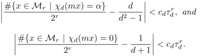
α∈ (Z/dZ)∗, r ∈ N ( ( ( (#{x ∈ Mr | χ2rd(mx) = α}− d d2− 1 ( ( ( ( < cdτdr, and ( ( ( (#{x ∈ Mr| χ2rd(mx) = 0} − 1 d + 1 ( ( ( ( < cdτdr.
Proof. See annex for the proof and the link with Stern sequences.
Taking m as the all zeros 160 bits vector, this asymptotic result let us think that the values χ(c) for c ∈ M0
160 are well distributed modulo d since (F162, d) =
(F163, d) = 1. In order to illustrate this theoretical result, we made several
nu-merical tests by generating all EAC of M0
n(from n = 10 to n = 29) and reducing
the corresponding integer modulo a n-bits prime number (recall that for a prac-tical use, we consider elements of M0
160 and a point P of order d about 2160).
Table 1 seems to show that even for chains whose length is much smaller than d, the distribution is not so bad. For each value of n, a random n-bits prime dn has
been generated. We have then computed for each α ∈ Z/dnZ, the cardinality
δα of χ−1(α) in M0n. Let T = {δα | α ∈ Z/dnZ}, for each t in T we have then
computed how many integers in [0, d − 1] are exactly computed t times. As an example, for t = 0 we know how many integers are never reached when reducing modulo d the value χ(c) for c ∈ M0
n.
5
A Second Family of EAC and an Open Problem
In order to generate a 160 bits integer, the author of [26] gives numerical results which show that the search for a chain whose length be less than 260 needs about 223 tests using a heuristic from Montgomery [32]. With such chains,
Al-gorithm 1 needs less multiplications than the classical SPA-resistant alAl-gorithms. We investigated the problem of choosing shorter chains in order to speed up the performances of algorithm 1. Once the length ( is fixed we have to deal with two constraints :
– the number p of 1’s in the chain must be chosen so that the greatest integer generated is as near as d ($ 2160) as possible,
– because of the non-injectivity of χ , %! p
&must be greater than 2160in order
to hope that the integers generated reach most of the elements of [1, 2160].
These two constraints lead us to study the sets M!,pwhere p < (/2.
Theorem 2. Let (p, () ∈ N2 such that 0 < 2p < (. Let F
i be the ith Fibonacci, αp= (1+ √ 2)p+(1 −√2)p 2 , βp= (1+√2)p −(1−√2)p 2√2 , then
i) For all m ∈ M!,p we have, F!−p+4+ pF!−p+2" χ(m) " F!−2p+4(αp+ βp)+
βpF!−2p+2.
ii) The lower bound is reached if and only if m = 1p0!−p or m = 0!−p1p.
iii) The upper bound is reached if and only if m = (01)p0!−2por m = 0!−2p(10)p.
Proof. See annex.
To improve the performances of Algorithm 1, we choose to use chains whose length is 240. In this case p = 80 seems to be the best choice with respect to our two constraints. With such parameters, we can randomly generate about 2216
chains computing integers in the interval [2117.7, 2158.9]. Unfortunately, it seems
to be a hard problem to compute the number of distinct integers generated in this way.
This naturally leads us to consider the set M3p,p. Numerical experiments for
some values of p let us think that the cardinality of χ(M3p,p) is near from 22p.
Notice that from the preceding theorem, it can be proved that the upper bound for ( = 3p is equivalent to γ%(1+√2)(1+√5) 2 &p where γ = (1+√5)4 32√5 + (1+√5)4 32√10 + (1+√5)2 8√10 which is close to γ2
1.96p. We end this section with an open problem :
What is the cardinality of χ(M3p,p) ? The good performances of this method
(see next section) make this problem of interest. Notice that a straightforward argument gives that the number of distinct integers generated (for the proposed parameters) is greater than 2106. Indeed, it follows from proposition 3 that the
chains 0120c, where c
∈ M120,80 give rise to distinct integers.
6
Comparisons
In this paper we have proposed three different ways to compute a point on the curve from an Euclidean addition chain :
Method 1: use a chain from M0
160for curves of order about 2224.
Method 2: use a chain from M0
160 for curves of order about 2160 even if χ(c)
can be greater than the order, using the results on Stern sequences. Method 3: use a chain from M240,80 for curves of order about 2160.
The interest of Method 1 is that it is the only method for which we have a proved security. The main drawback is that it forces us to work on curves defined over larger fields ($ 2224elements instead of 2160). However, we will see,
in Section 6.2, that it might not be such a problem in practical implementations. Moreover, this method shows to be particularly relevant in the context of fixed base point scalar multiplication.
Method 2 allows us to reduce the size of the underlying fields by using Stern’s results. Numerical samples tend to show that the generated keys are well dis-tributed but we still lack a complete security proof.
Finally, in Method 3, we try to reduce both the size of the fields and the length of the chains. In that case, it becomes very complicated to analyze the distribution of the generated keys. In particular, the system becomes highly redundant, which might lead to a bias in the set of possible chains. Typically, this would make this method irrelevant for signature and key-exchange schemes. We propose to compare our work to other side-channel resistant methods with a similar security level. We do not take into account special key generation meth-ods as they usually provide lower security level [33,34]. One could try to increase the size of the underlying field (as we do with Method 1) to solve this issue, however this would make those approaches slower than general algorithms. In the fixed point scenario, special key generation methods usually provide enough security but require in the same time a large amount of stored data: from 50 to 1000 precomputed points [15,4] when we only require a table of two stored points.
In Table 2, we summarize the cost, in terms of field multiplications, of various SPA-resistant scalar multiplication schemes providing a security of 80 bits. In order to ease comparisons, we make the traditional assumption that the cost of a field squaring (S) is 80 percent of that of a field multiplication (M).
Random Base Point. In that scenario, a new base point P is computed for each new session. This implies that it is not possible to precompute offline mul-tiples of P to speed up the process.
We consider the following SPA resistant methods:
– Dummy operations consist of adding a dummy point addition during the double-and-add algorithm, when the current bit is a 0.
– The Montgomery ladder is a SPA resistant algorithm from Peter Mont-gomery [31], performing one doubling and one addition for each bit of the scalar. It is only efficient on Montgomery curves.
– Unified formulae allow to perform doubling and addition with the same formulae on specific curve shapes. They can be then combined with the NAF representation for scalar multiplication. The cost of the unified operation is 11M, 12M and 14M on Edwards [2], Hessian [16] and Jacobi curves [23] respectively. We do not compare to Brier and Joye general unified formulae due to their quite high cost (18M) [5].
– M¨oller proposed a modified version of Brauer (2w-ary) algorithm [29]. Using
precomputations, its pattern is independent from the scalar itself. In that case, we used the latest and fastest point addition and point doubling formu-lae in Jacobian coordinates (see [1] for complete overview). One can also refer to the Left-to-Right recodings methods proposed in [39] whose performances are similar.
Fixed Base Point. In the context of a fixed base point we propose a new scalar multiplication scheme based on our chains generation method. Notice that in Methods 1 and 2, the 160 first steps of Algorithm 1 are fixed, independently of the scalar, and correspond to big steps. Hence we can precompute and store the points F162P and F163P and then generate random chains of length 160. We
compared these methods to the classical Comb method.
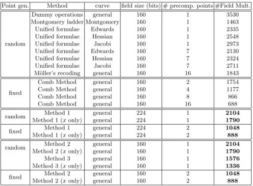
Table 2. Cost of various SPA resistant scalar multiplication methods providing 80 bits of security
Point gen. Method curve field size (bits) # precomp. points #Field Mult.
random
Dummy operations general 160 1 3530 Montgomery ladder Montgomery 160 1 1463 Unified formulae Edwards 160 1 2335 Unified formulae Hessian 160 1 2548 Unified formulae Jacobi 160 1 2973 Unified formulae Edwards 160 7 2130 Unified formulae Hessian 160 7 2324 Unified formulae Jacobi 160 7 2711 M¨oller’s recoding general 160 16 1843
fixed
Comb Method general 160 2 1754
Comb Method general 160 4 1177
Comb Method general 160 8 866
Comb Method general 160 16 688
random Method 1 general 224 1 2104
Method 1 (x only) general 224 1 1790
fixed Method 1 general 224 2 1048
Method 1 (x only) general 224 2 888
random Method 2 general 160 1 2104
Method 2 (x only) general 160 1 1790
Method 3 general 160 1 1576
Method 3 (x only) general 160 1 1336
fixed Method 2 general 160 2 1048
Method 2 (x only) general 160 2 888
To be completely fair, we evaluate in the next section the additional cost of working on larger fields with Method 1.
As for Method 2 and 3, Table 2 shows our different methods provide very good results. In the random point scenario, Methods 2 and 3 perform generally better that their counterparts. Only Montgomery’s algorithm can be claim to be faster, but its use is restricted to Montgomery’s curves. Besides, computing the x coordinate only with Method 3 leads to a faster scheme. In the fixed based point scenario, the Comb method requires at least 4 times more stored points to perform faster than our methods.
6.1 Comparison of Method 1 with Algorithms Working on 160-Bit Integers
Recall that Method 1 requires to work on fields of larger size (2224 elements).
Hence to be fair in our comparisons, we need to evaluate the additional cost of performing multiplications in larger fields. To this end, we are going to consider three contexts for modular multiplication. For each of them, we will identify scenarios for which it is worth using our method.
a) The CIOS method [21]: the Coarsely Integrated Operand Scanning method is an efficient implementation of Montgomery’s modular multiplication for a large class of processor. From [21] a modular multiplication between two in-tegers stored as s words of w bits needs 2s2+s w-bits multiplications, 4s2+4s+2
w-bits additions, 6s2+ 7s + 2 w-bits read instructions and 2s2+ 5s + 1 w-bits
write instructions. Using these results, we can estimate the cost in terms of w-bits operations of the methods listed in Table 2.This leads us to the following remarks.
On a 32 bits processor, for a random point P , Method 1 with x-only is the most performant SPA resistant method which can be used on any curve and which only stores the point P . For a fixed point P , if only two points can be stored, this latter is better than Comb method. On a 64 bits processor, the preceding remarks remain true. Moreover, the fixed point method (without the x coordinate trick) is competitive with the Comb method when only two points are stored. On a 128 bits processor, since two words are needed to store 160 bits integer or 224 bits integer, we only have to compare the number of field multiplications in Table 2. This shows that our method in the fixed point context is better than the Comb method when storing 2 or 4 points. For random point context, if one needs an SPA resistant algorithm which works on any curve and stores no more than one point, then our method gives the best result. b) The GNU multiprecision library: we provide benchmarks for fair comparisons between modular multiplications in the case of practical use with the library GMP. We compute several times 228modular multiplications (using
Table 3. Performances of Method 1 using CIOS method on 32 bits processor
s # Field mult. 32 bits× 32 bits + 32 bits Read 32 bits Write Method 1, x-only 7 1790 187950 404540 617550 239860
Dummy 5 3530 194150 430660 660110 268280 Method 1, fixed point, x-only 7 888 93240 200688 306360 118992 Comb method, 2 stored points 5 1754 96470 213988 327998 133304
Table 4. Performances of Method 1 using CIOS method on 64 bits processor
s # Field mult. 64 bits× 64 bits + 64 bits Read 64 bits Write Method 1, fixed point 4 1048 37728 85936 132048 55544 Comb method, 2 stored points 3 1754 36834 87700 135058 59636
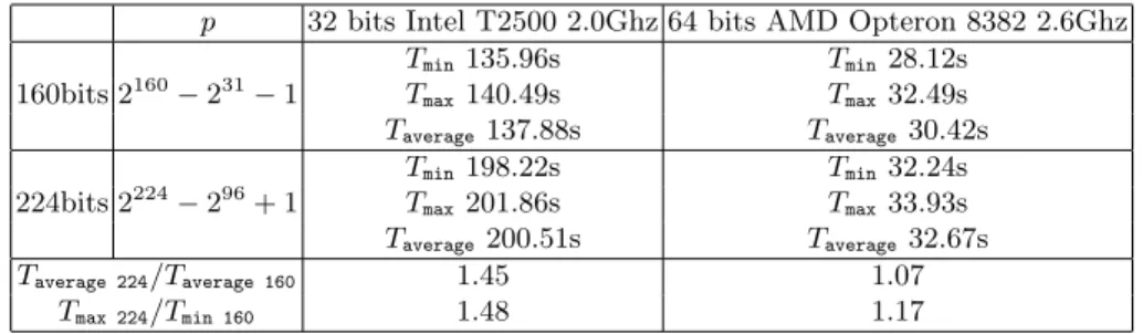
Table 5. Time to compute 228modular multiplications with GnuMP p 32 bits Intel T2500 2.0Ghz 64 bits AMD Opteron 8382 2.6Ghz
Tmin135.96s Tmin28.12s 160bits 2160− 231 − 1 Tmax140.49s Tmax32.49s Taverage137.88s Taverage30.42s Tmin198.22s Tmin32.24s 224bits 2224− 296+ 1 T max201.86s Tmax33.93s Taverage200.51s Taverage32.67s Taverage 224/Taverage 160 1.45 1.07 Tmax 224/Tmin 160 1.48 1.17
Table 6. Performances of Method 1 with GnuMP
Point gen. Method curve storage Mult. (32 bits proc.) Mult. (64 bits proc.) random Method 1 general 1 3114 2462
Method 1 (x only) general 1 2650 2095 fixed Method 1 general 2 1552 1227 Method 1 (x only) general 2 1315 1039
mpz mul and mpz mod) on 32 and 64 bits processors. We consider reduction modulo a prime number p conformant to the ANSI X9.63 standard [6] (resp. FIPS186-3 standard [40]) for the 160 bits (resp. 224 bits) case. From these benchmarks, we deduce an average time to compute a modular multiplication as detailed in table 5. Let us now consider the ratio in the most pessimistic case : the cost of a 224 bits modular multiplication is 1.17 times (resp. 1.48 times) the cost of a 160 bits multiplication for 64 bits (resp. 32 bits) processor. Taking into account these results, we can give an estimate in terms of 160 bits multiplications of Method 1. This shows the interest of Method 1, specially in the fixed point context (see table 2).
c) Hardware context: we considered in this section two kinds of com-ponents from the STMicroelectronics portfolio. The first embeds the Public Key 64 bits crypto processor from AST working at 200Mhz (CORE65LPHVT technology) and the second the 128 bits hardware smartcard cryptographic coprocessor Nescrypt working at 110Mhz. The AST crypto processor can compute about 2040816 160-bits modular multiplications and 1449275 224-bits modular multiplications per second. Taking into account these results, table 7 gives the time needed by the modular multiplications when computing a point multiplication. Once again, in the random point context, Method 1 obtains best performances if one needs an SPA resistant algorithm working on a general curve and storing only one point. In the fixed point context, Method 1 is faster than the Comb method with two points. Notice that we only consider the multiplications done by the cryptoprocessor for the times given in table 7. We do not take into account the overhead involved by the communications between the processor and the crypto processor.
Table 7. Time comparison for scalar multiplication methods in milliseconds Point gen. Method curve # precomp. points msecs
random (160 bits)
Dummy operations general 1 1.73
Montgomery ladder Montgomery 1 0.717 Unified formulae Edwards 1 1.144 Unified formulae Hessian 1 1.249
Unified formulae Jacobi 1 1.457
Unified formulae Edwards 7 1.044 Unified formulae Hessian 7 1.139
Unified formulae Jacobi 7 1.328
M¨oller’s recoding general 16 0.903
fixed (160 bits)
Comb Method general 2 0.859
Comb Method general 4 0.577
Comb Method general 8 0.424
Comb Method general 16 0.337
random (224 bits) Method 1 general 1 1.452
Method 1 (x only) general 1 1.235
fixed (224 bits) Method 1 general 2 0.723
Method 1 (x only) general 2 0.613
Nescrypt 128 bits crypto processor can compute about 339506 modular mul-tiplications per second both for 160 bits and 224 bits integers. Indeed in both cases, only two 128 bits blocks are used to manipulate these integers. Hence we can do the same remarks as in the section about the CIOS method.
7
Conclusions
The goal of this paper was to describe subsets of integers k for which the compu-tation of kP is faster, when dealing with the problem of SP A-secure exponenti-ation over an elliptic curve. We studied three such subsets and produced the first practical and theoretical results on random Euclidean addition chain generation. Table 2 shows that our methods provide good results in various situations when compared with the best SPA-secure methods.
We proved that the Method 1 we considered is secure and fast. In particular, in the context of a fixed base point, it is competitive with actual methods and faster when using similar amount of storage. We detailed several practical scenarios for which the method is relevant and improves efficiency : in CIOS context, in the context of GNU multiprecision library, and on some cryptoprocessors.
At last, we began the theoretical study of the other proposed methods. We made links between Method 2 and Stern sequences which enabled to obtain optimistic but asymptotic results. We managed to begin the study of the dis-tribution of integers generated by Method 3. Both methods would improve the performances once again. For example Method 3 would be faster than Mont-gomery ladder, thus it would be worth studying it further. We have proved some results that may be useful for any further investigation.
References
1. Bernstein, D.J., Lange, T.: Explicit-formulas database, http://hyperelliptic.org/EFD
2. Bernstein, D.J., Lange, T.: Faster addition and doubling on elliptic curves. In: Kurosawa, K. (ed.) ASIACRYPT 2007. LNCS, vol. 4833, pp. 29–50. Springer, Heidelberg (2007)
3. Bos, J.W., Kaihara, M.E., Kleinjung, T., Lenstra, A.K., Montgomery, P.L.: On the security of 1024-bit rsa and 160-bit elliptic curve cryptography. Technical report, EPFL IC LACAL and Alcatel-Lucent Bell Laboratories and Microsoft Research (2009)
4. Boyko, V., Peinado, M., Venkatesan, R.: Speeding up discrete log and factoring based schemes via precomputations (1998)
5. Brier, E., Joye, M.: Weierstraß elliptic curves and side-channel attacks. In: Nac-cache, D., Paillier, P. (eds.) PKC 2002. LNCS, vol. 2274, pp. 335–345. Springer, Heidelberg (2002)
6. Certicom Research. Sec 2: Recommended elliptic curve domain parameters stan-dards for efficient cryptography. Technical report, Certicom (2000)
7. Cohen, H., Frey, G., Avanzi, R., Doche, C., Lange, T., Nguyen, K., Vercauteren, F.: Handbook of Elliptic and Hyperelliptic Cryptography, Discrete Mathematics and its Applications, vol. 34. Chapman & Hall/CRC (2005)
8. Cohen, H., Miyaji, A., Ono, T.: Efficient elliptic curve exponentiation using mixed coordinates. In: Ohta, K., Pei, D. (eds.) ASIACRYPT 1998. LNCS, vol. 1514, pp. 51–65. Springer, Heidelberg (1998)
9. de Rooij, P.: On Schnorr’s preprocessing for digital signature schemes. In: Helle-seth, T. (ed.) EUROCRYPT 1993. LNCS, vol. 765, pp. 435–439. Springer, Hei-delberg (1994)
10. Dimitrov, V., Imbert, L., Mishra, P.K.: Efficient and secure elliptic curve point multiplication using double-base chains. In: Roy, B. (ed.) ASIACRYPT 2005. LNCS, vol. 3788, pp. 59–78. Springer, Heidelberg (2005)
11. Graham, R.L., Knuth, D.E., Patashnik, O.: Concrete Mathematics: A Foundation for Computer Science. Addison-Wesley, Reading (1989)
12. Hankerson, D., Menezes, A., Vanstone, S.: Guide to Elliptic Curve Cryptography. Springer, Heidelberg (2004)
13. Hisil, H., Koon-Ho Wong, K., Carter, G., Dawson, E.: Twisted Edwards curves revisited. In: Pieprzyk, J. (ed.) ASIACRYPT 2008. LNCS, vol. 5350, pp. 326–343. Springer, Heidelberg (2008)
14. Hoffstein, J., Silverman, J.H.: Random small hamming weight products with ap-plications to cryptography. Discrete Appl. Math. 130(1), 37–49 (2003)
15. M’Ra¨ıhi, D., Coron, J.-S., Tymen, C.: Fast generation of pairs (k, [k]p) for koblitz elliptic curves. In: Vaudenay, S., Youssef, A.M. (eds.) SAC 2001. LNCS, vol. 2259, pp. 151–174. Springer, Heidelberg (2001)
16. Joye, M., Quisquater, J.-J.: Hessian elliptic curves and side-channel attacks. In: Ko¸c, C¸ .K., Naccache, D., Paar, C. (eds.) CHES 2001. LNCS, vol. 2162, pp. 402– 410. Springer, Heidelberg (2001)
17. Kleinjung, T., Aoki, K., Franke, J., Lenstra, A.K., Thom´e, E., Bos, J.W., Gaudry, P., Kruppa, A., Montgomery, P.L., Osvik, D.A., te Riele, H., Timofeev, A., Zim-mermann, P.: Factorization of a 768-bit rsa modulus. Technical report, EPFL IC LACAL and NTT and University of Bonn and INRIA CNRS LORIA and Microsoft Research and CWI (2010)
18. Knuth, D., Yao, A.: Analysis of the subtractive algorithm for greater common divisors. Proc. Nat. Acad. Sci. USA 72(12), 4720–4722 (1975)
19. Knuth, D.E.: The Art of Computer Programming: Fundamental Algorithms, 3rd edn, vol. 2. Addison Wesley, Reading (July 1997)
20. Koblitz, N.: CM-curves with good cryptographic properties. In: Feigenbaum, J. (ed.) CRYPTO 1991. LNCS, vol. 576, pp. 279–287. Springer, Heidelberg (1992) 21. Koc, C.K., Acar, T.: Analyzing and comparing montgomery multiplication
algo-rithms. IEEE Micro 16, 26–33 (1996)
22. Kocher, P., Jaffe, J., Jun, B.: Differential power analysis. In: Wiener, M. (ed.) CRYPTO 1999. LNCS, vol. 1666, pp. 388–397. Springer, Heidelberg (1999) 23. Liardet, P.-Y., Smart, N.P.: Preventing SPA/DPA in ECC systems using the
Jacobi form. In: Ko¸c, C¸ .K., Naccache, D., Paar, C. (eds.) CHES 2001. LNCS, vol. 2162, pp. 391–401. Springer, Heidelberg (2001)
24. Longa, P., Gebotys, C.: Setting speed records with the (fractional) multibase non-adjacent form method for efficient elliptic curve scalar multiplication. In: Jarecki, S., Tsudik, G. (eds.) Public Key Cryptography – PKC 2009. LNCS, vol. 5443, pp. 443–462. Springer, Heidelberg (2009)
25. Longa, P., Miri, A.: New composite operations and precomputation scheme for elliptic curve cryptosystems over prime fields. In: Cramer, R. (ed.) PKC 2008. LNCS, vol. 4939, pp. 229–247. Springer, Heidelberg (2008)
26. Meloni, N.: Arithm´etique pour la Cryptographie bas´ee sur les Courbes Elliptiques. PhD thesis, Universit´e de Montpellier, France (2007)
27. Meloni, N.: New point addition formulae for ECC applications. In: Carlet, C., Sunar, B. (eds.) WAIFI 2007. LNCS, vol. 4547, pp. 189–201. Springer, Heidelberg (2007)
28. Mironov, I., Mityagin, A., Nissim, K.: Hard instances of the constrained discrete logarithm problem. In: Hess, F., Pauli, S., Pohst, M. (eds.) ANTS 2006. LNCS, vol. 4076, pp. 582–598. Springer, Heidelberg (2006)
29. M¨oller, B.: Securing elliptic curve point multiplication against side-channel at-tacks. In: Davida, G.I., Frankel, Y. (eds.) ISC 2001. LNCS, vol. 2200, pp. 324–334. Springer, Heidelberg (2001)
30. M¨oller, B.: Improved techniques for fast exponentiation. In: Lee, P.J., Lim, C.H. (eds.) ICISC 2002. LNCS, vol. 2587, pp. 298–312. Springer, Heidelberg (2003) 31. Montgomery, P.: Speeding the pollard and elliptic curve methods of factorization.
Mathematics of Computation 48, 243–264 (1987)
32. Montgomery, P.L.: Evaluating recurrences of form Xm+n = f (Xm, Xn, Xm−n)
via Lucas chains (1992), http://ftp.cwi.nl/pub/pmontgom/Lucas.ps.gz 33. Mui, J.A., Stinson, D.R.: On the low hamming weight discrete logarithm problem
for nonadjacent representations. Applicable Algebra in Engineering, Communica-tion and Computing 16, 461–472 (2006)
34. Nguyˆen, P.Q., Stern, J.: The hardness of the hidden subset sum problem and its cryptographic implications. In: Wiener, M. (ed.) CRYPTO 1999. LNCS, vol. 1666, pp. 31–46. Springer, Heidelberg (1999)
35. Reznick, B.: Regularity properties of the stern enumeration of the rationals. Jour-nal of Integer Sequences 11 (2008)
36. Schnorr, C.P.: Efficient signature generation by smart cards. Journal of Cryptol-ogy 4, 161–174 (1991)
37. Stern, M.A.: ¨uber eine zahlentheoretische funktion. Journal f¨ur die reine und angewandte Mathematik 55, 193–220 (1858)
38. Stinson, D.R.: Some baby-step giant-step algorithms for the low hamming weight discrete logarithm problem. Mathematics of Computation 71, 379–391 (2000)
39. Theriault, N.: Spa resistant left-to-right integer recodings. In: Preneel, B., Tavares, S. (eds.) SAC 2005. LNCS, vol. 3897, pp. 345–358. Springer, Heidelberg (2006) 40. U.S. Department of Commerce and National Intitute of Standards and
Technol-ogy. Digital signature standard (DSS). Technical report (2009)
41. Yacobi, Y.: Exponentiating faster with addition chains. In: Damg˚ard, I.B. (ed.) EUROCRYPT 1990. LNCS, vol. 473, pp. 222–229. Springer, Heidelberg (1991) 42. Yacobi, Y.: Fast exponentiation using data compression. SIAM J. Comput. 28(2),
700–703 (1999)
Annex
Proof of Theorem 1
Definition 3. Let (a, b) ∈ N2, the generalized Stern sequence
(sa,b(r, n))r∈N,n∈[0,2r] is defined by sa,b(0, 0) = a, sa,b(0, 1) = b, and for r! 1,
sa,b(r, 2n) = sa,b(r − 1, n), sa,b(r, 2n + 1) = sa,b(r − 1, n) + sa,b(r − 1, n + 1).
In his original paper, Stern gave a practical description of his sequence using the following diatomic array [37] :
(r = 0) a b (r = 1) a a + b b
(r = 2) a 2a + b a + b a + 2b b
(r = 3) a 3a + b 2a + b 3a + 2b a + b 2a + 3b a + 2b a + 3b b ...
where each line r is exactly the sequence sa,b(r, n) for n ∈ [0, 2r]. Notice that
to compute the row r, you just have to rewrite row r − 1 and insert their sum between two elements. In the case (a, b) = (1, 1), the sequence is called the Stern sequence and has been well studied. For example, see the introduction of [35] or [11] for the link with the Stern Brocot array.
Now we will point deep connections between Stern sequences and the ψ and χ maps. These connections should not surprise us, because both are linked with continued fractions. As an example, if (a, b) = (1, 1), an easy induction enables us to prove that when n ∈ [0, 2r[, the sequence (s
1,1(r +1, 2n), s1,1(r +1, 2n+1))
describes the set ψ(Mr).
(r = 0) 1 1 (r = 1) 1 2 1 (r = 2) 1 3 2 3 1 (M2= { 00, 01, 10, 11}) (r = 3) 1 4 3 5 2 5 3 4 1 (ψ(M2) = { (3, 5), (2, 5), (3, 4), (1, 4)}) ... Let us note ∆ : N2
→ N2such that ∆(x, y) = (y, x). Another induction enables
to prove that when n ∈ [0, 2r+1− 1], (s
1,1(r + 1, n), s1,1(r + 1, n + 1)) describes
ψ(Mr) ∪ ∆(ψ(Mr)). For ( ∈ N∗ and m ∈ M!, let Ar(m) = {ψ(mx) | x ∈
From now on, in order to simplify the notations, we will denote by s(r, n) the value sa,b(r, n). Let us define the sequences %S(r, n)&r∈N,n∈[0,2r−1] by
S(r, n) = (s(r, n), s(r, n + 1)) and%Sd(r, n)&r∈N,n∈[0,2r−1] by Sd(r, n) = (s(r, n)
mod d, s(r, n + 1) mod d). The following link between ψ and S can be proved by induction.
Lemma 1. Let r ! 0, ( > 0 and let m ∈ M! such that ψ(m) = (a, b). Then
S(r + 1, .) is a one to one map from [0, 2r+1
− 1] onto Ar(m).
It means that in our case, the values ψ(c) and ∆(ψ(c)) for c ∈ M0
! correspond
to the elements S(( + 1, n) for n ∈ [0, 2!+1
− 1] and (a, b) = (F!+2, F!+3).
Re-cently, Reznick proved in [35] that, for d! 2, (a, b) = (1, 1), and r sufficiently large, the sequence {Sd(r, n)}n∈N is well distributed among Sd := {(i mod d, j
mod d) | gcd(i, j, d) = 1}. We need a similar result for any couple (a, b) in order to show that the values χ(c) are asymptotically well distributed modulo d. We will use similar notations and follow the arguments of [35] to prove the next theorem. We define :
– for γ ∈ Sd, Bd(r, γ) := #{n ∈ [0, 2r− 1] |Sd(r, n) = γ},
– χd, the map such that χd(m) = χ(m) mod d,
– ψd the map such that if ψ(m) = (v, u) then ψd(m) = (v mod d, u mod d),
– Nd the cardinality of Sd.
Theorem 3. Let (a, b, d) ∈ N3 such that d be prime and (a, d) = (b, d) = 1.
There exist constants cd and ρd < 2 so that if m∈ N and α ∈ Sd, then for all
r! 0, |Bd(r, α) − 2r Nd| < cd ρr d.
Proof. Due to the lack of space, we just give a short proof of this, following the arguments of section 4 in [35] and pointing out the differences. Since d is prime, we have Sd = Z/dZ × Z/dZ \ {(0, 0)}, and Nd = d2− 1. We can define a graph
Gdand the applications L and R in the same way, and also have Ld = Rd = id.
In the proof of lemma 14, we have to give a slightly different proof that for each α = (x, y)∈ Sdthere exists a way from (a, b) to α in the graph Gd. Notice that since
(0, 0) +∈ Sd, then either x += 0 or y += 0. If y += 0, we notice that Rk
!
(Lk(a, b)) =
(a + k#(b + ka), b + ka). As (a, d) = 1, we can choose k such that b + ka = y.
Thus, as y += 0, we can choose k# such that a + k#(b + ka) = x and we are done.
If x += 0, then we consider Lk!(Rk(a, b)) = (a + kb, b + k#(a + kb)) : in the same
way, we can choose (k, k#) such that a + kb = x and b + k#(a + kb) = y. In the first
line of the proof of lemma 14, we also have to consider (r0, n0) ∈ N × N such that
Sd(r0, n0) = (0, 1) rather than Sd(0, 0) = (0, 1). Thus the adjacency matrix of
the graph satisfies the same properties as in theorem 15 of [35]. So the conclusion remains true for Bd.
Proof. Let α ∈ (Z/dZ)∗, and (β
i, γi)1!i!d the d elements of Z/dZ × Z/dZ \
{(0, 0)} such that βi+ γi = α, then
#{x ∈ Mr| χd(mx) = α} =)di=1#{x ∈ Mr| ψd(mx) = (βi, γi)}.
If n ∈ [0, 2r+1] is such that S
d(r + 1, n) = (βi, γi) then , thanks to Lemma 1,
it corresponds to x ∈ Mr such that ψd(mx) = (βi, γi) or ψd(mx) = (γi, βi). In
this last case, there exists an integer j, such that (γi, βi) = (βj, γj). Hence, d * i=1 #{n ∈ [0, 2r+1 −1] | Sd(r +1, n) = (βi, γi)} = 2×#{x ∈ Mr| χd(mx) = α}. Now by definition of Bd : d * i=1 #{n ∈ [0, 2r+1 − 1] | Sd(r + 1, n) = (βi, γi)} = d * i=1 Bd(r + 1, (βi, γi)). Thus, #{x ∈ Mr| χd(mx) = α} 2r − d d2− 1 = d * i=1 "B d(r + 1, (βi, γi)) 2r+1 − 1 d2− 1 # . Then we can use Theorem 3 and the triangular inequality to prove the first inequality of the theorem. Using this inequality for α += 0 we prove the second inequality.
Proof of Theorem 2
From now on, we will denote by m, the value χ(m). Let us set M = sup {m | m ∈ M!,p} and I = inf {m | m ∈ M!,p}. If m ∈ M!,p is not one of the words of
the points ii) (resp. iii)), we will propose m# ∈ M
!,p such that m# < m (resp.
m# > m). The lemmas in the two following subsections give the details about
the words m# we use to compare.
We first look for m ∈ M!,psuch that m = I. First suppose that two 1’s in the
word m are separated by one 0 or more. Then we can consider (m, n, s) ∈ (N∗)3
and (a, b) ∈ N2 and (x, y) ∈ M
a× Mb such that m is one of the words
1m0n1s, x10m1n0y or y01n0m1x.
We won’t consider the third case because it is the symmetric of the second one. The lemma 2 shows that 1m0n1s> 1m+s0n and that x10m1n0y > x1n+10m+1y.
So if m = I, there are no 0 between two 1 of the word m, and so there are integers a and c such that m = 0a1p0c. From lemma 3 we show that a = 0 (and
so c = ( − p) or c = 0 (and so a = ( − p).
Now we look for m ∈ M!,p such that m = M. If there are two consecutive
1’s in the word m, as 2p < ( the word m will also have two consecutive 0’s. We can consider the symmetry such that a subword 00 appears in m before a subword 11. In this case there exists (a, b, n) ∈ N3 and (x, y) ∈ M
that m = x00(10)n11y. In this case, we have from lemma 4 that m < x(01)n+2y.
Now assume that there are no subword 11 in m. If two 1’s in the word m are separated by two 0’s or more, then there exists (m, n, a, b) ∈ (N∗)2
×N2, x ∈ M a
and y ∈ Mb such that m is one of the words
x010n(01)m, x010n(01)m0, x010n(01)m02y, 10n(01)m, 10n(01)m0, or 10n(01)m02y.
The Lemmas (5) and (6) give us in any case m# ∈ M
!,p such that m < m#.
We have just proved that 11 is not a subword of m, and that two 1’s of m are separated by exactly one 0. So the word m or its symmetric is 0a(01)p0c where
(a, c) ∈ N×N. The lemma (7) shows that M is reached when a = 0 (so c = (−2p) or when c = 1 (so a = ( − 2p − 1). Then the point iii) is proved.
Now we just have to apply Proposition 1 to deduce i) from ii) and iii). Lemmas to Find the Lower Bound
Lemma 2. Let (m, n, s) ∈ (N∗)3 and (a, b) ∈ N2. Let x ∈ M
a and y ∈ Mb. We
have
i) 1m0n1s > 1m+s0n and
ii) x10m1n0y > x1n+10m+1y.
Proof. For the point i) , we compute 1m0n1s= (1, 2) "1 m 0 1 # " Fn−1 Fn Fn Fn+1 # "1 s 0 1 # "1 1 # , so 1m0n1s= (s + 1)F n−1+%(s + 1)(m + 2) + 1&Fn+ (m + 2)Fn+1. (2) Also, 1m+s0n= (1, 2) "1 m + s 0 1 # " Fn−1 Fn Fn Fn+1 # "1 1 # , so 1m+s0n= (2 + m + s + 1)F n+1+ (2 + m + s)Fn. (3)
The difference between (2) and (3) is msFn, so it is positive in the conditions
of the lemma. We can notice that there is equality when s = 0 or when m = 0, which can also be explained by the symmetry.
To prove the point ii), let us set (v, u) = ψ(x). We have ψ(x10m1n0) = (v, u) "1 1 0 1 # " Fm−1 Fm Fm Fm+1 # "1 n 0 1 # "0 1 1 1 #
=%(nFm+Fm+1)u+(nFm+1+Fm+2)v, Fm+2u+(Fm+1+(n+1)Fm+2)v +(u−v)nFm&.
(4) We also compute ψ(x1n+10m+1) = (v, u) "1 n + 1 0 1 # " Fm Fm+1 Fm+1Fm+2 #
= (Fm+1u + (Fm+ (n + 1)Fm+1)v, Fm+2u + (Fm+1+ (n + 1)Fm+2)v). (5)
As u > v, we can deduce the point ii) from the comparison components by components of the vectors (4) and (5).
Lemma 3. Let (a, b, c) ∈ (N∗)3, we have 0a1b0c > 1b0a+c.
Proof. We first compute the left hand side 0a1b0c= (1, 2) " Fa−1 Fa Fa Fa+1 # "1 b 0 1 # " Fc−1 Fc Fc Fc+1 # "1 1 #
= (Fa+2Fc−1+ (bFa+2+ Fa+3)Fc+ Fa+2Fc+ (bFa+2+ Fa+3)Fc+1+)
= Fa+2Fc+1+ Fa+3Fc+2+ bFa+2Fc+2. (6)
We also compute the right hand side 1b0a+c= (1, 2) "1 b 0 1 # " Fa+c−1 Fa+c Fa+c Fa+c+1 # "1 1 # = (Fa+c−1+ (b + 2)Fa+c+ Fa+c+ (b + 2)Fa+c+1)
= Fa+c+4+ bFa+c+2.
With eq. 1, page 242 we show that it is
Fa+2Fc+1+ Fa+3Fc+2+ bFa+c+2. (7)
The difference between (6) and (7) is b(Fa+c+2− Fa+2Fc+2) = bFcFa, which is
positive in the conditions of the lemma. In the cases c = 0 or a = 0, there is equality which we already knew by the symmetry.
Lemmas to Compute the Upper Bound Lemma 4. Let (n, a, b) ∈ N3. For all x ∈ M
a and y ∈ Mb we have
x00(10)n11y < x(01)n+2y.
Proof. We first compute S02(S1S0)nS12= "1 1 1 2 # " αn 2βn βn αn # "1 2 0 1 # ="αn+ βn 3αn+ 4βn αn+ 2βn4αn+ 6βn # . We set (v, u) = ψ(x), so we have ψ(x00(10)n11) = (v, u) " αn+ βn 3αn+ 4βn αn+ 2βn4αn+ 6βn # = (v(αn+ βn) + u(αn+ 2βn), v(3αn+ 4βn) + u(4αn+ 6βn)) . (8)
From the other hand S0S1(S0S1)nS0S1= "0 1 1 2 # " αn− βn βn βn αn+ βn # "0 1 1 2 # = " αn+ βn 2αn+ 3βn 2αn+ 3βn 5αn+ 7βn # , so ψ(x(01)n+2) = (v(αn+ βn) + u(2αn+ 3βn), v(2αn+ 3βn) + u(5αn+ 7βn)) . (9)
As v < u we can compare the vectors (8) and (9) components by components and then conclude.
Lemma 5. Let (m, n, a, b) ∈ (N∗)2 × N2. For all x ∈ M a and y ∈ Mb, we have i) x010n(01)m < x(01)m+10n ii) x010n(01)m0 < x(01)m+10n+1 iii) x010n(01)m02y < x(01)m+10n+2y. Proof. We compute S0S1S0n= "0 1 1 2 # " Fn−1 Fn Fn Fn+1 # =" Fn Fn+1 Fn+2Fn+3 # . We deduce S0S1S0n(S0S1)m= " Fn Fn+1 Fn+2Fn+3 # " αm− βm βm βm αm+ βm # and so S0S1S0n(S0S1)m= " αmFn+ βmFn−1 αmFn+1+ βmFn+2 αmFn+2+ βmFn+1αmFn+3+ βmFn+4 # . (10)
From the other hand, we can write (S0S1)m+1S0n = (S0S1)mS0S1S0n so
(S0S1)m+1S0n= " αm− βm βm βm αm+ βm # " Fn Fn+1 Fn+2Fn+3 # , and then (S0S1)m+1S0n= " αmFn+ βmFn+1 αmFn+1+ βmFn+2 αmFn+2+ βm(Fn+ Fn+2) αmFn+3+ βm(Fn+1+ Fn+3) # (11) Let us set (v, u) = ψ(x). ψ(x010n(01)m) = (v, u) " αmFn+ βmFn−1 αmFn+1+ βmFn+2 αmFn+2+ βmFn+1αmFn+3+ βmFn+4 # "1 1 # = v(αmFn+2+ βmFn−1+ βmFn+2) + u(αmFn+4+ βmFn+1+ βmFn+4). (12) We also have ψ(x(01)m+10n) = (v, u) ! αmFn+ βmFn+1 αmFn+1+ βmFn+2 αmFn+2+ βm(Fn+ Fn+2) αmFn+3+ βm(Fn+1+ Fn+3) " ! 1 1 "
= v(αmFn+2+ βmFn+1+ βmFn+2) + u(αmFn+4+ βmFn+2+ βmFn+4). (13)
The difference between (13) and (12) is vβmFn+ uβmFn so we deduce the first
point.
To prove the point ii) we use (10) which gives S0S1Sn0(S0S1)mS0= " αmFn+1+ βmFn+2αmFn+2+ βmFn−1+ βmFn+2 αmFn+3+ βmFn+4αmFn+4+ βmFn+1+ βmFn+4 # (14)
Let us set (v, u) = ψ(x). We have x010n(01)m0 = v(α mFn+3+ βmFn−1+ 2βmFn+2) +u(αmFn+5+ βmFn+1+ 2βmFn+4). (15) From (11) we deduce (S0S1)m+1S0n+1= " αmFn+1+ βmFn+2 αmFn+2+ βmFn+3 αmFn+3+ βmFn+1+ βmFn+3αmFn+4+ βmFn+2+ βmFn+4 # (16) So x(01)m+10n+1= v(αmFn+3+ βmFn+4) + u(αmFn+5+ βmFn+3+ βmFn+5). (17)
The difference between (17) and (15) is vβmFn so we have the positivity. To
prove iii) we compute from (14) and (16) S0S1S0n(S0S1)mS20= ! αmFn+2+ βmFn−1+ βmFn+2αmFn+3+ βmFn−1+ 2βmFn+2 αmFn+4+ βmFn+1+ βmFn+4αmFn+5+ βmFn+1+ 2βmFn+4 " and (S0S1)m+1Sn+20 = ! αmFn+2+ βmFn+3 αmFn+3+ βmFn+4 αmFn+4+ βmFn+2+ βmFn+4αmFn+5+ βmFn+3+ βmFn+5 " . We compare components by components and then deduce iii)
Lemma 6. Let (m, n, b) ∈ (N∗)2× N and y ∈ M
b. We have
i) 10n(01)m < (01)m+10n−1,
ii) 10n(01)m0 < (01)m+10n,
iii)10n(01)m02y < (01)m+10n+1y.
Proof. We will use the computations of the proof of lemma 5. Let us consider that ψ(x) = (1, 1). In this case ψ(x0) would be (1, 2), and we would have x010n(01)m= 10n(01)m. So with (12) we have
10n(01)m= α
With (11) we have
(01)m+10n−1= αmFn+1+ βmFn+ βmFn+1+ 2αmFn+3+ 2βmFn+1+ 2βmFn+3,
(19) so (01)m+10n−1− 10n(01)m= α
mFn−1+ βmFn+2, and then we have the point
i) . In the same way, we also have 10n(01)m0 = α
mFn+3+βmFn−1+2βmFn+2+αmFn+5+βmFn+1+2βmFn+4, and
(01)m+10n= α
mFn+2+βmFn+1+βmFn+2+2αmFn+4+βmFn+2+βmFn+4, so
(01)m+10n− 10n(01)m0 = F
n(αm+ 2βm) and then we deduce the point ii) .
Now, ψ(10n(01)m02) = (1, 1)S
0S1S0n(S0S1)mS02, and with (15) we find
ψ(10n(01)m02) = (α m(Fn+2+ Fn+4) +βm(Fn−1+ Fn+5), αm(Fn+3+ Fn+5) + βm(Fn−1+ Fn+5)). (20) With (11) we compute ψ((01)m+10n+1) = (α m(Fn+1+ 2Fn+3) + βm(Fn+1+ 3Fn+3), αm(Fn+2+ 2Fn+4) + βm(Fn+2+ 3Fn+4). (21)
The difference of the first component of (21) by the first component of (20) is αmFn−2+ βmFn+2, and the difference of the second components is αmFn +
βm(2Fn+4− Fn−1− Fn+1) so the point iii) is proved.
Lemma 7. Let (a, b, c) ∈ N × N∗× N. If c += 1 and a += 0 then 0a(01)b0c <
(01)b0a+c. Proof. We compute 0a(01)b0c= (1, 2) " Fa−1 Fa Fa Fa+1 # " αb− βb βb βb αb+ βb # " Fc−1 Fc Fc Fc+1 # "1 1 #
= αb(Fa+2Fc+1+ Fa+3Fc+2) + βb(Fa+1Fc+1+ Fa+4Fc+2). (22)
On the other hand (01)b0a+c= (1, 2) " αb− βb βb βb αb+ βb # " Fa+c−1 Fa+c Fa+c Fa+c+1 # "1 1 #
= αbFa+c+4+ βb(Fa+c+2+ Fa+c+4). (23)
Using eq. 1, we prove that the difference between (23) by (22) is βbFa(Fc+1−Fc).