HAL Id: lirmm-01589007
https://hal-lirmm.ccsd.cnrs.fr/lirmm-01589007
Submitted on 18 Sep 2017
HAL is a multi-disciplinary open access
archive for the deposit and dissemination of
sci-entific research documents, whether they are
pub-lished or not. The documents may come from
teaching and research institutions in France or
abroad, or from public or private research centers.
L’archive ouverte pluridisciplinaire HAL, est
destinée au dépôt et à la diffusion de documents
scientifiques de niveau recherche, publiés ou non,
émanant des établissements d’enseignement et de
recherche français ou étrangers, des laboratoires
publics ou privés.
Formal Method for Mission Controller Generation of a
Mobile Robot
Silvain Louis, Karen Godary-Dejean, Lionel Lapierre, Thomas Claverie,
Sébastien Villéger
To cite this version:
Silvain Louis, Karen Godary-Dejean, Lionel Lapierre, Thomas Claverie, Sébastien Villéger. Formal
Method for Mission Controller Generation of a Mobile Robot. TAROS: Towards Autonomous Robotic
Systems, Jul 2017, University of Surrey, Guildford, United Kingdom. pp.586-600,
�10.1007/978-3-319-64107-2_48�. �lirmm-01589007�
Formal method for mission controller generation
of a mobile robot
Silvain Louis1,2, Karen Godary-Dejean1, Lionel Lapierre1, Thomas Claverie2,3,
and S´ebastien Vill´eger2,3
1 LIRMM, University of Montpellier, France
{name}@lirmm.fr
2 MARBEC, CUFR Mayotte, France
3 MARBEC, CNRS, Montpellier, France
Abstract. This article presents a methodology for generating a real-time mission controller of a submarine robot. The initial description of the mission considers the granularity constraints associated with the ac-tors defining the mission. This methodology incorporates a formal analy-sis of the different possibilities for success of the mission from the models of each component involved in the description of the mission. This article ends illustrating this methodology with the generation of a real robotic mission for marine biodiversity assessment.
Keywords: Formal analysis, Mission controller, Mobile robot
1
Introduction and context
One of the current major challenges of ecology, is to protect biodiversity against increasing threats from human activities (e.g. climate change, fishing). Towards this aim the first, and critical, step is to be able to assess biodiversity in as many places and as often as possible. Compared to terrestrial ecosystems, marine ecosystems are still poorly known because underwater observation of marine organisms by divers is a demanding task. Indeed, divers could not operate for more than one hour especially in deep habitats (i.e. > 20m) while counting mobile, abundant and diverse animals such as fishes required a long training. In addition presence of divers could affect the behavior of animals (attractive or repulsive interactions) which could ultimately bias biodiversity assessments.
MARBEC laboratory aims to address the challenge of assessing marine bio-diversity in temperate and tropical coastal areas to ultimately provide conser-vation guidelines for their sustainable exploitation. Roboticians from LIRMM have been working for several years on the design of a semiautonomous robot named Ulysse able of performing underwater missions as video-recording mis-sions. Ulysse is a submarine robot with 12 vector thrusters so that it is holo-nomic. It is autonomous in energy and carries its control architecture on an embedded computer. It receives remote orders through a cable connected to a
surface computer. It incorporates multiple sensors such as an inertial unit (IMU) and a Doppler loop sensor (DVL). It has a front live-camera for help with piloting and 2 front-top cameras for recording stereo-videos of marine organisms.
Researchers from LIRMM and MARBEC laboratories start an interdisci-plinary scientific collaboration to improve observation techniques of marine bio-diversity. The aim is to transpose live-census diver-operated protocols commonly used to monitor fish biodiversity, to a video-recording robot-based approach. Transect protocol [1] consists in censusing all fishes along a virtual segments of 50m length at a constant depth. Localized observation consists in observing an habitat of interest (e.g. coral patch) from different angles. From a robotic point of view, we defined the 2 protocols as operating modes, each with different control algorithms. The robot is co-controlled, with some actions autonomously controlled while others are remotely driven by human operator. In the case of the Transect, the robot is controlled by a linear path (given depth and orien-tation) along which it is allowed to rotate around a vertical axis (to simulate the rotation of the diver head). In the case of localized observation, the robot control performs centering around the point of interest and the robot can only rotate at a fixed distance around it (i.e. on a sphere).
Therefore, a robot must be able to perform complex, modular and easily constructable missions. Such missions includes different users with very differ-ent skills, with differdiffer-ent point of view and differdiffer-ent needs. On the robotic side, each element of the mission must contain, to face with complex and unknown environment, functional, algorithmic, sensory or actuating redundancy. The con-struction of the mission controller and its formal verification must take all these aspects into account. To achieve this, we present in this article a methodology of generation and verification of the mission controller, based on a semi-formal language for mission description.
We will begin by presenting the needs of modularity and granularity for biologists and how this impacts the description of the architecture. Then, we present the mission description, voluntarily simplified to suit our partners. Then, we present the associated formal models and the methodology of generation and validation of the mission controller. Finally, we illustrate the methodology on a real example of mission.
2
Control architecture levels
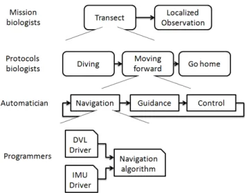
The main concern of our architectural description in the context of the collabo-ration between roboticians and on-the-field experts (here, biologists) is that each actor can best exercise his competences at an appropriate level of abstraction. Thus the biologists could need two different views. First, on the field, responsible for the mission, they must have the vision of the whole mission and the possibility to change of protocols at any time. Here, they do not need knowing the technical details of the protocols implementation. But before that, the biological protocols must be stated more precisely into several high level robotic tasks. Studying the effectiveness of protocols, biologists also need to modify the mission parameters
and to create new protocols without having to rewrite the robotic control laws, and without being dependent on the missions using these protocols. Then, auto-maticians, in charge of the control laws, must be able to write the appropriated control laws of the robotic tasks without being constrained by the utilization context of these laws. In the lowest level of abstraction, programmers, in charge of the implementation of the control architecture on the execution target, do not need to have a global vision of the missions, but must precisely manage the implementation constraints. These different levels of abstraction can be summa-rized in Figure 1.
Fig. 1. Abstraction levels of the mission description
The integration of a mission into an architecture must consider 3 main parts: a decisional part, an automatic algorithmic part and a specific part to the im-plementation on the middleware. In this article, we will concentrate particularly on the decisional part of our methodology without neglecting the constraints related to the algorithm part and the implementation.
3
State of the art
To answer our problematic, we have sought in the literature, a formal model-ing language, allowmodel-ing a hierarchical and modular description. It must also be complete but simple. This formalism should also be easily interfaced with the current architecture of our experimental platform.
We can find UML [2], composed of 13 diagrams (The package diagram, the use case diagram, the activity diagram ...) depending on the desired modeling
but UML is not formal. We must also mention the Battle Management Lan-guage (BML) used to command and control forces and equipment conducting military operations [3] but BML is not modular enough in our context. We can find Language grammar, explain in [4] and partially used in [2] but which are hierarchically not simple. There is also XML, use in [5] (with XPath query lan-guage) and that we also use in the high-level description of our description for its simplicity of utilization and its great description flexibility. The XML language is not formal, but we use it only for the mission description and not for the verification.
We have also turned to programming languages since our mission will have to be executed on a real robot. In the synchronous languages, we quote the Esterel language [6], which is imperative and modular, allowing the instantaneous dif-fusion of signals. We will cite the RMPL (Reactive Model-Based Programming Language) [7] which allows model-based programming, used by NASA (DS1 probe). I would also quote the Signal [8] [9], Luster [10] and StateChart [11] lan-guage. All these synchronous languages do not allow a formal verification with a hierarchical description. In asynchronous languages, I will quote the BIP (Behav-ior Interaction Pr(Behav-iority) language of the LAAS architecture based on the use of component and allowing the formal validation [12] [13]. The dataflow associated with the BIP language allows to generate code executing on their architecture (Realtime BIP Engine) but which is incompatible with the architecture of our Ulysse robot.
There is very often the use of several representations within the same struc-ture, it is also our case, as explained below.
4
Mission description
These works are in collaboration with those of Benoit Ropars on the hierarchiza-tion within an architecture [14] as well as those of Lotfi Jaiem on an approach for hardware and software resources management [15].
To answer the needs expressed in section 2, we have defined a hierarchical de-scription of the mission through 3 elements described in XML: Objective blocks, Parallel blocks and Activities.
4.1 Objective block
The Objective block (Fig. 2) has an entry point and two exit points (Success and Failure). The block is activated when a token arrives at its entry point. If the objective succeeds, it sends a token on its success exit point. If the objective fails, the token go on the failure exit point. There are 2 types of objectives: Recursive objectives and Elementary objectives. Recursive objectives are encapsulations of a series of lower level objectives. It is therefore possible to build a complex mission using objective decomposition. The elementary objectives are the lowest level of decomposition. The highest objective block is the stand alone block named Mission block. The entry point of the Mission block is activated at the start of the robot.
Fig. 2. Objective block
4.2 Parallel block
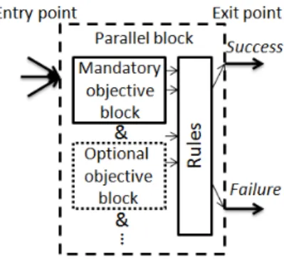
The Parallel block (Fig. 3) allows several objectives to be performed at the same time (for example, a motion objective and a measurement objective). It has the same entry and exit points as the objective block. The parallel block has an objectives list that may be mandatory or optional. There is necessarily at least one mandatory objective per Parallel block. When activated, the Parallel block activates all its internal objectives. When all the internal objectives are completed, the choice of the final exit point value (Success or Failure) follows these rules: the success of all mandatory objectives drives the success of the Parallel block, conversely a failure of a mandatory objective causes its failure.
Fig. 3. Parallel block
4.3 Activity, alternative and resource
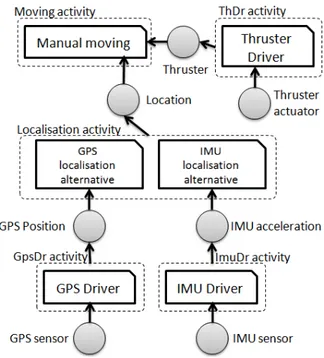
The activities are present in the Elementary objectives. They allow to carry out the basic robotic tasks (e.g. Location, Control, Guidance ...). An activity comes in several alternatives which are the different possibilities to perform the associ-ated robotic task. For example, in our robot, the Localisation activity can have 2 alternatives: Location by GPS (active when the robot is on the surface) and
Location by IMU integration (always possible). All the alternatives of a unique activity are ordered by priority. For example, the 2 location alternatives have a priority order which corresponds to the location accuracy. Activities provide resources (e.g. the Location value) and consume resources, which may be dif-ferent depending on the selected alternative (GPS position in the case where the alternative GPS localisation alternative is selected or IMU position in the case where the alternative IMU localisation alternative is selected, in the example of Fig. 4).
For example, in Figure 4 we see a Manual control objective with 5 ac-tivities and 7 resources. All acac-tivities have only one alternative, except the Localisation activity, which has 2. The GpsDr activity will only be active if the GPS localisation alternative of the Localisation activity is selected (same principle for the activity ImuDr). There are therefore two functioning modes for the architecture to achieve the Manual control objective.
Fig. 4. Activities of the Manual control objective
Resources are divided into 2 categories: software resources and hardware resources. The software resources are produced by the activities. They are gen-erally data carrier (for example the coordinates X and Y of the robot location resource). The hardware resources represent a real object in virtual form in the robot architecture, mostly associated to a sensor (for example the acoustic space around the robot) or a actuator (for example a thruster).
For a given elementary objective, all the possible combination of alternatives, with their associated resources production and consumption, form the different possible control schemes of the robot to perform this objective. The sequences of all the combination of all the objectives of a mission are called functioning modes (detailed below).
5
Methodology
When the mission is completely defined through the description of the objectives blocks, we apply the methodology summarized below to generate the mission controller embedded on the robot. All these steps are automatically performed by the generation program, except the formal analysis (see below).
5.1 Objectives graph
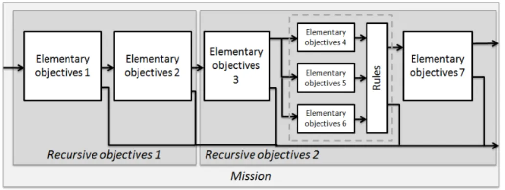
At this point in the description of the mission, we have objectives on several levels of description. The first step consists in replacing all recursive objective blocks and parallel blocks with their contents to get a single level with only ele-mentary objectives. The result of this flattening is called the Objectives Graph. An example of such a graph is given Fig. 5.
Fig. 5. Mission flattening
5.2 Alternatives graph
It is necessary to generate the mission controller, which will pilot the control algorithms of the robot. To do this, we must deduce all the possible combina-tions of control according to the different activities, alternatives and resources presented in the model of the mission. To extract these combinations, it is nec-essary to be able to represent the links between all these elements. To do this,
we have decided to use a formal language representation in order to study all the possible state space and thus the possible states of our controller.
There are several modeling languages as SMV (Symbolic model checking) [16], timed automata [17] or Petri net [5]. In our methodology, we will use the Petri network. Indeed, this validation language is particularly adapted for the discrete event system as our mission description. The possibility of modeling the parallelism of two subsystems and their synchronization is adapted to model the resources, the activities, the objectives and the connections between them.
6
Petri net models
We describe the internal behavior and the interface of each block in Petri nets. We also model the activities and their resources, and the links of production / consumption. Then we can rewrite the whole mission as a complete Petri nets model.
6.1 Resources models
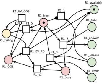
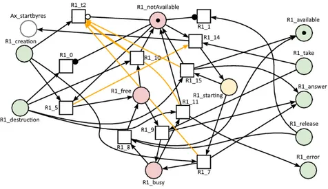
In both the software (Fig. 7) and hardware (Fig. 6) Petri net models of resources, the internal structure (i.e. the common states Rx free and Rx busy) is repre-sented by places (in red on the figures). In addition, hardware resources have an internal state Rx OOS corresponding to the out-of-service (OOS in this article) state of this resource. Software resources have an internal state Rx notAvailable when the activity that produces this resource is not in execution.
The transition represent the evolution between these states, either because all the input places of the transition are marked with a token, or if a specific event occurs (Rx EV yy). Resource models also represent temporary states of resources (in orange on the figures). In the hardware resource model, there is a failing temporary state triggered by the Rx EV OOS event. Conversely, there is the event Rx EV RD if the resource is available again. The resources do not have the Rx EV OOS and Rx EV RD events because they are conditioned only by their activity which produces them and therefore can not be physically OOS.
Unlike hardware resources, software resources do not exist when the activity that produces is not in execution. The resource must be created (activation place) and destroyed (deactivation place) on the order of the activity. It must wait for the activity to start (waiting place). All possible states of waiting, activation and deactivation of the producing resource are represented by internal states.
Fig. 7. Software resource Petri net model
Places could also represent the production/consumption interface (in green on the figures). The interface of resources is divided into 5 places. The place Rx available indicates to the activity that wants to consume the resource that the resource is available. The place Rx take allows the request to reserve the resource. The place Rx answer allows the consuming activity to know that the resource has answered to the request, whereas the place Rx release allows to release the resource. Finally, the place Rx error allows to notify the consuming activity if the producing activity stops producing the resource. This happens after the occurrence of the Rx EV OOS event.
6.2 Activities models
We also model the activities by Petri net with the alternatives that compose it. There are 2 ways to start an activity. Either directly from the Start interface which comes from the modeling of the objectives. In this case, the stop is made by the interface Stop. Or from the StartByRes interface when a resource, produced by the activity, is requested. In this case, the stop is performed when no resource produced by this activity is requested.
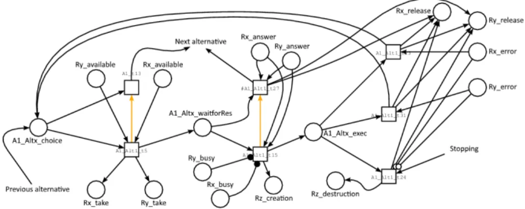
Once the activity is launched, all the conditions (consumed resources avail-able) of the alternatives will be evaluated according to their priority orders. If all the conditions are good, then the alternative is selected, the consumed re-sources are reserved and the produced rere-sources are activated. An alternative stops when the activity is stopped or when a resource error occurs, in which case all alternatives are re-evaluated. See Fig. 8, the model of a single alterna-tive branch. If no alternaalterna-tive is possible, then the activity generates an error to the mission controller.
Fig. 8. Alternative branch Petri net model
6.3 Mission models
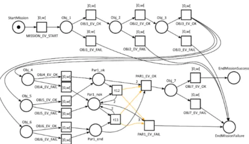
We transform the objectives graph into Petri net. The events OBJx EV OK and OBJx EV FAIL are issued by the activities within the objective. In addition to the places corresponding to the objectives, there is an initial place corresponding to the beginning of the mission with a transition on the event MISION EV START as well as 2 final places in case of success or failure of the mission. We have modeled the parallel blocks differently than the objectives to comply with the output rules, see 4.2. In Fig 9, the transformation of the objective graph (Fig. 5) into a Petri net is shown.
Fig. 9. Exemple of a mission Petri net model
7
Mission controller
7.1 Controller generation
Once the models of the different blocks are integrated and linked together, we perform an analysis to construct the markings graph. It represents the entire state space of the Petri net. In our case, it represents all the combinations (i.e. all the functioning modes) for each objective throughout the mission.
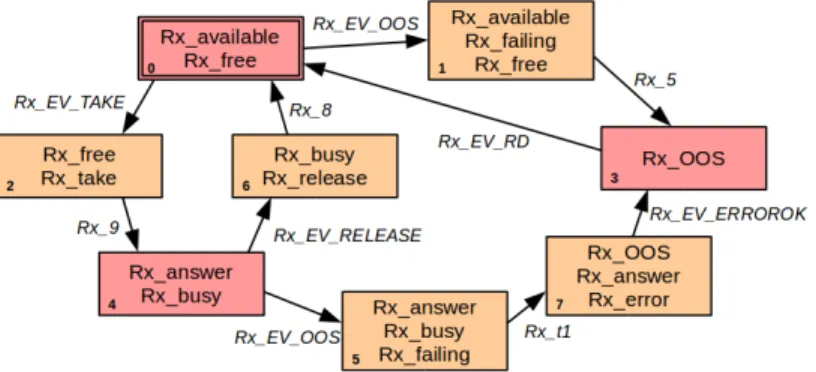
We see in Fig. 10 the markings graph of a hardware resource (i.e. of the Petri net of Fig. 6). The states contains the marking of the system at a given instant. In the example of Fig. 10, consider that the system is in its initial state with two marked places: Rx available and Rx free. The reservation of this hardware resource will be represented by the modification of the marking of the places of its interface. To simulate that, we add here a transition, associated to the event Rx EV TAKE, which consumes the token of the place R1 available and marked the place Rx take4. Firing this transition Rx EV TAKE, the system moves to the state with the marking free/take. Then, from this state, the transition Rx 9 place the system in the state answer/busy. And so on, constructing the entire marking graph. In all models, transitions associated with events are given lower priority than other transitions.
In this graph, we observe two types of states: the stable states (in red on the figure) which are the states really achievable by the system, and the transient states (in orange on the figure) which are only present in the graph due to the
4
The events Rx EV RELEASE and Rx EV ERROROK are also only present in the example to simulate the release of the resource
Fig. 10. Markings graph of a hardware resource
modelling process, which could need extra transitions firing to represent a change of states. Considering again the preceding example, States 0, 3 and 4 are real states of the resource, whereas states 1, 2, 5, 6 and 7 are only due to internal evolution of the model. Stable states are identified because they have always and exclusively exit transitions with events (* EV *). Also, due to the construction of the Petri net models, the firing from a state of one event always leads to a deterministic stable state. Thus, if we are interested only on the real resource possible states, we could simplify the markings graph by keeping only the stable states. The simplified graph of the markings graph of Fig. 10 is given Fig. 11.
Fig. 11. Simplified marking graph of a hardware resource
On the same principle as the previous example of the resource, we generate the markings graph of the global Petri net model, i.e. all the models of the activ-ities (with their alternatives), resources, mission objectives (from the objective graph) and all the connections between them. The stable states of the mark-ings graph give the robot’s functioning modes throughout the mission with the resources state and the alternatives selected of each activity.
7.2 Feasibility analysis
From the markings graph, we can perform formal analyzes. We can analyze that the system is live (no deadlock in the mission) and bounded (no modeling
mistake leading to an infinite state space). We can also verify specific functional properties, as for example that the place corresponding to the success of the mission is reachable. These analysis are done using a model checker on the states space of the system, here the markings graph. It is thus possible to do advanced analyzes, for example studying the resource events that force the mission into a branch leading to failure.
7.3 Controller implementation
Robot architecture is based on the real-time middleware ContrACT. ContrACT is composed of synchronous modules (ordered in a control loop), a scheduler and asynchronous modules (execute on events). Activities are coded in synchronous modules. The alternatives are segments of code in the synchronous modules (executed according to a parameter input). The mission controller is encoded in an asynchronous module. The mission controller receives the events * EV * and reads in the graph of the alternatives the actions he must perform (alter-native change, activation / deactivation of activity). The mission controller is automatically generated from the alternatives graph as a finite state machine.
8
Application example
We have applied this methodology for a realistic mission planned by our biologist partners. The mission is the study of a coral zone, first performing a localized observation of a specific coral head and then performing a transect from the coral head to a given heading. The localized observation has 2 lower level el-ementary objectives: Manual moving, to go to the head of coral, followed by Isopheric observation. The transect begins with the objective Diving, then Filming, Advancing and Measuring temperature in parallel and ending with Going up to the surface. This mission is similar to the one shown figure 5, with 7 elementary objectives, 3 of which are in parallel. The whole mission com-prises 11 activities (thruster driver, gps driver, imu driver, localisation, manual moving, isopheric observation, diving, filming, advancing, temperature, go surface). The activity localisation has 2 alternatives (gps localisation, imu localisation). There are 7 resources: 3 hardware (GPS sensor, IMU sensor, thruster actuator) and 4 software (GPS position, IMU acceleration, location, thruster). We consider that all the hardware resources may be faulty, but the software resources can not.
First we have generated the whole Petri nets model of the mission. The model a too complex to be shown here, but its size in terms of numbers of places and transition is given in the column 1 of Table 1, as well as the duration necessary for this generation. Once the mission model has been generated, we have generated the markings graph using the tool Tina [18], a classical tool used for the generation of the state space of (possibly time) Petri net models. The toolbox tina also contains, among others useful tools, a model checker which allows LTL property verification. The markings graph generation results (size
and generation duration) for our example model are given column 2 of Table 1. Finally, we have simplified the markings graph (automatically done by our program) to generate the alternatives graph and the mission controller. The results are given in the 3rd column of table 1.
Table 1. Model and graphs generation results Petri nets Generation time 0.24s Places no. 133 Transitions no. 150 Markings graph Generation time 116s States no. 819111 Transitions no. 1907422 Alternatives graph Generation time 191s States no. 765 Transitions no. 3602
Thanks to this methodology, we have generated a mission controller (from the alternatives graph) ready to operate. This controller could react to the failure of a resource, managing the expected changing of functioning mode.
9
Conclusion
In this article, we have presented an architecture allowing different actors to define their part of the mission with an adapted level of abstraction. We have provided the necessary blocks for the description of the mission, in a semi-formal language automatically translated into a formal model (using Petri nets). We have presented the formal methodology related to this architecture allowing to study the accessibility properties of the success of the mission. This methodology also allows the study of the different functioning modes ensuring the control of the robot to fulfill the objectives. Finally, we have generated the mission controller that allow the online control of the robot at the decisional level.
The rest of this work will study how to reduce the alternatives graph to limit the risk of combinatorial explosion in case of complex architecture and mission. One idea could be to locally consider the objectives, or the parallel sections, gen-erating local graph dedicated to each objective instead of gengen-erating a complete graph for the whole mission. We are also working on more reliable dependability methods (FMECA, risk analysis, fault tolerance..) and thus refining the fault models, their detection and the recovery after a failure.
Acknowledgment
The authors graciously thank the CUFR, FEDER, NUMEV and Agglo Beziers Mediterranee for their support to this work.
References
1. G. J. Edgar, N. S. Barrett, and A. J. Morton, “Biases associated with the use of underwater visual census techniques to quantify the density and size-structure of
fish populations,” Journal of Experimental Marine Biology and Ecology, vol. 308, no. 2, pp. 269–290, 2004.
2. F. Adolf and F. Andert, “Onboard Mission Management for a VTOL UAV Using Sequence and Supervisory Control,” in Cutting Edge Robotics 2010, 2010, pp. 301– 317.
3. NATO and RTO, “Coalition Battle Management Language ( C-BML ),” Tech. Rep., 2012.
4. A. Meduna, Formal Languages and Computation: Models and Their Applications. CRC Press, 2014.
5. E. Fern´andez-Perdomo, J. Cabrera-G´omez, A. C. Dom´ınguez-Brito, and D. Hern´andez-Sosa, “Mission specification in underwater robotics,” Journal of Physical Agents, vol. 4, no. 1, pp. 25–34, 2010.
6. G. Berry and G. Gonthier, “The Esterel Synchronous Programming Language: Design, Semantics, Implementation,” Science Of Computer Programming, 1992. 7. M. Ingham, R. Ragno, and B. C. Williams, “A reactive model-based programming
language for robotic space explorers,” Proceedings of ISAIRAS-01, 2001.
8. H. Marchand, ´E. Rutten, M. Le Borgne, and M. Samaan, “Formal verification of programs specified with signal: application to a power transformer station con-troller,” Science of Computer Programming, vol. 41, no. 1, pp. 85–104, 2001. 9. H. Marchand, P. Bournai, M. Le Borgne, and P. Le Guernic, Synthesis of discrete
controllers based on the signal Environment. Boston, MA: Springer US, 2000, pp. 479–480.
10. N. Halbwachs, P. Caspi, P. Raymond, and D. Pilaud, “The synchronous data flow programming language LUSTRE,” Proceedings of the IEEE, vol. 79, no. 9, pp. 1305–1320, 1991.
11. D. Harel, “Statecharts: a visual formalism for complex systems,” Science of Com-puter Programming, vol. 8, no. 3, pp. 231–274, 1987.
12. A. Basu, S. Bensalem, M. Bozga, J. Combaz, M. Jaber, N. Thanh-Hung, and J. Sifakis, “Rigorous Component-Based System Design Using the BIP Framework,” IEEE Software, vol. 28, pp. 41–48, 2011.
13. A. Basu, L. Mounier, M. Poulhi`es, J. Pulou, and J. Sifakis, “Using BIP for modeling and verification of networked systems - A case study on TinyOS-based networks,” Proceedings - 6th IEEE International Symposium on Network Computing and Ap-plications, NCA 2007, pp. 257–260, 2007.
14. B. Ropars, A. Lasbouygues, L. Lapierre, and D. Andreu, “Thruster’s dead-zones compensation for the actuation system of an underwater vehicle,” in ECC: Euro-pean Control Conference, Linz, Austria, Jul. 2015.
15. L. Jaiem, L. Lapierre, K. GodaryDejean, and D. Crestani, “Toward Performance Guarantee for Autonomous Mobile Robotic Mission: An Approach for Hardware and Software Resources Management,” in TAROS’16, Sheffield, UK, 2016. 16. J. R. Burch, E. M. Clarke, K. L. McMillan, D. L. Dill, and L. J. Hwang, “Symbolic
model checking: 1020 States and beyond,” Information and Computation, vol. 98, no. 2, pp. 142–170, 1992.
17. R. Alur, “Timed Automata,” University of Pennsylvania, Tech. Rep., 1998. 18. B. Berthomieu, P. O. Ribet, and F. Vernadat, “The tool tina–construction of
ab-stract state spaces for petri nets and time petri nets,” International journal of production research, vol. 42, no. 14, pp. 2741–2756, 2004.