HAL Id: halshs-00186905
https://halshs.archives-ouvertes.fr/halshs-00186905
Submitted on 13 Nov 2007
HAL is a multi-disciplinary open access
archive for the deposit and dissemination of
sci-entific research documents, whether they are
pub-lished or not. The documents may come from
teaching and research institutions in France or
L’archive ouverte pluridisciplinaire HAL, est
destinée au dépôt et à la diffusion de documents
scientifiques de niveau recherche, publiés ou non,
émanant des établissements d’enseignement et de
recherche français ou étrangers, des laboratoires
Dominance of capacities by k-additive belief functions
Pedro Miranda, Michel Grabisch, Pedro Gil
To cite this version:
Pedro Miranda, Michel Grabisch, Pedro Gil.
Dominance of capacities by k-additive belief
functions.
European Journal of Operational Research, Elsevier, 2006, 175 (2), pp.912-930.
�10.1016/j.ejor.2005.06.018�. �halshs-00186905�
Dominance of capacities by k-additive belief functions
∗
Pedro Miranda
†Universidad Complutense de Madrid
Plaza de Ciencias, 3, 28040 Madrid, Spain
pmiranda@mat.ucm.es
Michel Grabisch
Universit´e Paris I-Panth´eon-Sorbonne
LIP6 8, rue du Capitaine Scott, 75015 Paris
Michel.Grabisch@lip6.fr
Pedro Gil
Universidad de Oviedo
c/ Calvo Sotelo s/n, 33007 Oviedo, Spain
pedro@pinon.ccu.uniovi.es
Abstract
In this paper we deal with the set of k-additive belief functions dominating a given capacity. We follow the line introduced by Chateauneuf and Jaffray for dominating probabilities and continued by Grabisch for general k-additive measures. First, we show that the conditions for the general k-additive case lead to a very wide class of functions and this makes that the properties obtained for probabilities are no longer valid. On the other hand, we show that these conditions cannot be improved. We solve this situation by imposing additional constraints on the dominating functions. Then, we consider the more restrictive case of k-additive belief functions. In this case, a similar result with stronger conditions is proved. Although better, this result is not completely satisfactory and, as before, the conditions cannot be strengthened. However, when the initial capacity is a belief function, we find a subfamily of the set of dominating k-additive belief functions from which it is possible to derive any other dominant k-additive belief function, and such that the conditions are even more restrictive, obtaining the natural extension of the result for probabilities. Finally, we apply these results in the fields of Social Welfare Theory and Decision Under Risk.
Keywords: Linear programming, decision analysis, capacity, dominance, k-additivity, belief functions.
1
Introduction
The problem of finding the set of probabilities dominating a capacity has been extensively studied; for instance, Dempster [3] and Shafer [25] have proposed a representation of uncertainty based on a “lower probability” or “degree of belief”, respectively, to every event. Their model needs a lower probability function, usually non-additive but having a weaker property: monotonicity of order k, for all k, i.e. it is a belief function [25]. This requirement is perfectly justified in some situations (see [3]). The general form of lower probabilities has been studied by several authors (see e.g. [31, 32]).
Moreover, in many decision problems, in which we have not enough information, decision makers often feel that they are only able to assign an interval value for the probability of events. In other words, the real probability distribution is unknown, but there exists a set of probabilities compatible with the available information. Let us call this set of all compatible additive probabilities P1 and let us define µ := infP∈P1P ; then, µ is a capacity
(but not necessarily a belief function [30]); µ is called “coherent lower probability”, and it is the natural “lower
∗This paper is a revised and extended version of [19], presented at IFSA2003 conference.
†Corresponding author: Pedro Miranda. Dept. of Statistics and O.R. Universidad Complutense de Madrid. Address: Plaza
de Ciencias, 3, Ciudad Universitaria, 28040, Madrid (Spain). Tel: (+34) 91 394 43 77. Fax: (+34) 91 394 44 06. e-mail: pmi-randa@mat.ucm.es
probability function”. Of course, if P′is a probability distribution dominating µ, it is clear that E
P′(f ) ≥ Cµ(f ),
for any function f , where Cµrepresents Choquet integral [2] (function f plays the role of an action in the Decision
problem [27]). Chateauneuf and Jaffray use in [1] this fact and that µ ≤ P, ∀P ∈ P1 to obtain an easy method
to compute infP∈P1EP(f ). This method is based on the set of all probability distributions dominating µ. The
same can be done for obtaining an upper bound.
In our case, we try to extend these results for k-additive measures. There are some cases where this could be useful. First, suppose a situation that can be modelled by a k-additive measure (an axiomatic approach to this situation can be found in [17, 22]), but where our information does not allow us to completely determine the measure. Then, we have to work with a set of compatible k-additive measures (let us call it Uk). A second
example is the identification of a capacity in a practical situation. It can be proved that sometimes it is not possible to determine a single solution but a set of k-additive measures, all equally suitable [16]; it can also be proved that the set of all suitable measures is a convex set and consequently, the measure for an event A ⊆ X can take an interval of possible values (a deeper study about the unicity of solution and the structure of the set of solutions can be found in [20]). If µ = infµk∈Ukµk, then µ is clearly a capacity [27], and we have the
inequality Cµ′
k(f ) ≥ Cµ(f ), for any k-additive measure µ ′
k dominating µ and for any function f . Therefore, it
seems interesting to find the set of all k-additive fuzzy measures dominating µ in order to try to translate the results in [1]. However, we will see later that the results for the general k-additive case are too weak to deal with. Thus, we will focus on the special case of belief functions.
The paper is organized as follows: In next section we introduce the basic concepts on fuzzy measures that we will use in the paper. In Section 3 we recall the results on dominating probabilities and k-additive measures. We also show that the conditions for the k-additive case are too general in order to maintain the good properties derived for probabilities; we finish the section showing that these conditions are nevertheless necessary. In Section 4 we treat the problem of obtaining the set of dominating k-additive belief functions dominating a capacity. Section 5 is devoted to the applications in decision making. We finish with the conclusions and open problems.
2
Basic concepts on non-additive measures
Consider a finite referential set of n elements (criteria in Multicriteria Decision Making, players in Cooperative Games, incomes in Welfare Theory, ...), X = {1, ..., n}. The set of subsets of X is denoted by P(X), while the set of subsets whose cardinality is less or equal than k is denoted by Pk(X). Subsets of X are denoted A, B, .... We
will sometimes write i1· · · ik instead of {i1, . . . , ik} in order to avoid heavy notation; brackets are usually omitted
for singletons and subsets of two elements.
In order to be self-contained, we introduce the concepts that will be needed throughout the paper.
Definition 1. A non-additive measure [4] or fuzzy measure [27] or capacity [2] over (X, P(X)) is a mapping µ : P(X) → [0, 1] satisfying
• µ(∅) = 0, µ(X) = 1 (boundary conditions).
• ∀A, B ∈ P(X), if A ⊆ B, then µ(A) ≤ µ(B) (monotonicity).
In the sequel, we will mainly use the word ”capacity”. We denote the set of all capacities over X by FM(X). An important class of capacities is the following:
Definition 2. A unanimity game over A ⊆ X, A 6= ∅ is a capacity defined by
uA(B) :=
½
1 if A ⊆ B 0 otherwise For ∅, we define the unanimity game by
u∅(B) :=
½
1 if B 6= ∅ 0 if B = ∅
Definition 3. [5] Let µ be a capacity. We say that µ is k-monotone (for k ≥ 2) if and only if for any family of k subsets A1, ..., Ak of X, µ( k [ j=1 Aj) ≥ X ∅6=I⊆{1,...,k} (−1)|I|+1µ(\ j∈I Aj).
If µ is k-monotone for all k ≥ 2, then it is said that µ is a belief function. We will denote by BEL(X) the set of all belief functions on X.
There are other set functions that can be used to equivalently represent a capacity. In this paper we will need the so-called M¨obius transform.
Definition 4. [24] Let µ be a set function (not necessarily a non-additive measure) on X. The M¨obius trans-form (or inverse) of µ is another set function on X defined by
m(A) := X
B⊆A
(−1)|A\B|µ(B), ∀A ⊆ X.
The M¨obius transform given, the original set function can be recovered through the Zeta transform [1]: µ(A) = X
B⊆A
m(B).
The value m(A) represents the strength of the subset A in any coalition in which it appears. The M¨obius transform corresponds to the basic probability mass assignment in Dempster-Shafer theory of evidence [25].
The M¨obius transform can be applied to any set function. Given a M¨obius inverse, necessary and sufficient conditions for obtaining a proper capacity have been investigated. The following can be proved:
Proposition 1. [1] A set of 2n coefficients m(A), A ⊆ X, corresponds to the M¨obius transform of a capacity if
and only if (i) m(∅) = 0, X A⊆X m(A) = 1. (ii) X i∈B⊆A
m(B) ≥ 0, for all A ⊆ X, for all i ∈ A.
In particular, (ii) implies that m(i) ≥ 0, ∀i ∈ X. Related to unanimity games and belief functions, the following result can be proved:
Proposition 2. [12, 25]
• The M¨obius transform of the unanimity game on A, with A 6= ∅, is given by
m(B) = ½
1 if B = A 0 otherwise
For u∅, the M¨obius inverse is given by m(A) = (−1)|A|+1, ∀A ⊆ X, A 6= ∅ and m(∅) = 0.
• µ is a belief function if and only if its corresponding M¨obius inverse is non-negative.
In order to determine a capacity, 2n− 2 values are necessary. The number of coefficients grows exponentially
with n and so does the complexity of the problem of identification. This drawback reduces considerably the practical use of non-additive measures. In an attempt to reduce complexity, some subfamilies of non-additive measures have been defined e.g. k-additive measures [9], p-symmetric measures [18], k-intolerant measures [15], λ-measures [28], or more generally decomposable measures [6]. In this paper we will consider k-additive measures. Definition 5. [9] A non-additive measure µ is said to be k-order additive or k-additive if its M¨obius transform vanishes for any A ⊆ X such that |A| > k and there exists at least one subset A with exactly k elements such that m(A) 6= 0.
In this sense, a probability measure is just a 1-additive measure [9]. Thus, k-additive measures generalize probability measures, that are very restrictive in many situations as they do not allow interactions between the elements of X. They fill the gap between probability measures and general non-additive measures. For a k-additive measure, the number of coefficients is reduced to
k X i=1 µn i ¶ .
More about k-additive measures can be found e.g. in [10]. We will denote the set of all k′-additive measures
with k′ ≤ k on X by FMk(X); in particular, FM1(X) represents the set of all probability distributions.
Analogously, the set of all k′-additive belief functions, with k′ ≤ k on X is denoted by BELk(X). Remark that
FM1(X) = BEL1(X).
Definition 6. Consider a capacity µ. We say that a capacity µ∗ dominates µ, and we denote it µ∗≥ µ, if and
only if
µ∗(A) ≥ µ(A), ∀A ⊆ X.
Given a capacity µ, the set of all k-additive (at most) capacities dominating µ will be denoted by FMk ≥(µ).
The set of all k-additive (at most) belief functions dominating µ will be denoted by BELk≥(µ). It is trivial to see from Definition 6 that FMk≥(µ) (resp. BELk≥(µ)) is a convex polyhedron and, consequently, it is characterized by its vertices. The set of vertices is called the profile.
Let Σ be the set of all permutations on X; given σ ∈ Σ, let us denote by Xl
σ, 0 ≤ l ≤ n, the subset of X defined
by
Xσl := {σ(1), ..., σ(l)}, l ≥ 1, Xσ0= ∅.
Definition 7. Given a capacity µ, we denote by FMkΣ(µ) (resp. BELkΣ(µ)) the subset of FMk(X) (resp.
BELk(X)) containing the capacities (resp. belief functions) µ∗ satisfying
∃σ ∈ Σ | ∀l = 1, ..., n, µ∗(Xl
σ) = µ(Xσl).
3
Dominating probabilities versus dominating k-additive measures
Let us now start our study. Chateauneuf and Jaffray have studied in [1] the problem of dominating a capacity by probabilities. They obtain the following result:
Theorem 1. Let µ be a capacity on X, m its M¨obius transform, and suppose P ∈ FM1≥(µ). Then, P can be
put under the following form:
P ({i}) =X
B∋i
λ(B, i)m(B), ∀i ∈ X,
and P (A) =P
i∈AP ({i}) for any A ⊆ X. The function λ : P(X) × X → [0, 1] is a weight function satisfying:
X
i∈B
λ(B, i) = 1, ∀B ⊆ X.
λ(B, i) = 0 whenever i 6∈ B.
Dempster has shown the same result in [3] and also Shapley in [26], but both of them only for belief functions. Grabisch has extended Theorem 1 for the k-additive case. He proved the following result:
Theorem 2. [13] Let µ be a capacity on X, m its M¨obius transform and suppose that µ∗ ∈ FMk
≥(µ). Then,
necessarily, the M¨obius transform m∗ of µ∗ can be put under the following form:
m∗(A) = X
B∩A6=∅
where function λ : P(X) × Pk(X) → R is such that
X
A|B∩A6=∅
λ(B, A) = 1, ∀B ⊆ X. (1)
λ(B, A) = 0, ∀A ∈ Pk(X), A ∩ B = ∅. (2)
In the following, the set function obtained for a given choice of λ in the conditions of Theorem 2 will be denoted by µλ and mλ its corresponding M¨obius transform.
At first sight, Theorem 2 is a straight generalization of Theorem 1 and both results are very similar. However, there are two important facts related to λ that should be kept in mind:
• λ in Theorem 2 can attain negative values, while in Theorem 1 it is a weight function.
• The condition B ∋ i of Theorem 1 can be generalized in two different ways for general subsets: A ⊆ B and A ∩ B 6= ∅. The second case includes the first one. It must be remarked that in Theorem 2 the second alternative is used.
These two conditions are necessary for the general k-additive case and cannot be simplified, as the following examples show:
Example 1. [13] Let us start showing that A ⊆ B instead of A ∩ B 6= ∅ in Equations (1) and (2) does not suffice to recover all k-additive measures dominating µ. Consider |X| = 3 and the fuzzy measure defined by:
{1} {2} {3} {1, 2} {1, 3} {2, 3} {1, 2, 3} m 0.1 0.1 0.1 0.1 0.2 0.2 0.2 µ 0.1 0.1 0.1 0.3 0.4 0.4 1 Let us consider now the belief function defined by:
{1} {2} {3} {1, 2} {1, 3} {2, 3} {1, 2, 3} m∗ 0.35 0.1 0.1 0 0 0.45 0
µ∗ 0.35 0.1 0.1 0.45 0.45 0.65 1
Then, µ∗ ≥ µ and µ∗is 2-additive, but in the sharing procedure, if we change A ∩ B by A ⊆ B, m∗(2, 3) should
be derived only from m(2, 3) and m(1, 2, 3). But then, m(2, 3) + m(1, 2, 3) = 0.4 < m∗(2, 3) = 0.45, and therefore
no sharing function would lead to µ∗.
Example 2. Let us now show that λ may attain negative values. Consider |X| = 3 and again the capacity µ defined in Example 1. Let us take now the 2-additive measure defined by:
{1} {2} {3} {1, 2} {1, 3} {2, 3} {1, 2, 3} m∗ 0.7 0.3 0.2 -0.2 0 0 0
µ∗ 0.7 0.3 0.2 0.8 0.9 0.5 1
Thus, µ∗≥ µ but m∗(1, 2) < 0 and then we need a function λ taking negative values.
The following notations will be useful to shed light on the differences between these two theorems: Λk∩:= {λ : P(X) × Pk(X) → R | ∀B ∈ P(X), X A∩B6=∅ λ(B, A) = 1, λ(B, A) = 0 if A ∩ B = ∅}. Λk∩,+:= {λ : P(X) × Pk(X) → [0, 1] | ∀B ∈ P(X), X A∩B6=∅ λ(B, A) = 1, λ(B, A) = 0 if A ∩ B = ∅}. Λk ⊆,+:= {λ : P(X) × Pk(X) → [0, 1] | ∀B ∈ P(X), X A⊆B λ(B, A) = 1, λ(B, A) = 0 if A 6⊆ B}.
Given µ ∈ FM(X) whose corresponding M¨obius transform is m, we define MΛk ∩(µ) := {µλ| mλ(A) = X B∈P(X) λ(B, A)m(B), λ ∈ Λk ∩}. MΛk ∩,+(µ) := {µλ| mλ(A) = X B∈P(X) λ(B, A)m(B), λ ∈ Λk∩,+}. MΛk ⊆,+(µ) := {µλ| mλ(A) = X B∈P(X) λ(B, A)m(B), λ ∈ Λk ⊆,+}.
With this notation, MΛ1
⊆,+(µ) is the set of functions in the conditions of Theorem 1 and MΛk∩(µ) represents the
set of functions obtained by Theorem 2.
For these families, Grabisch has studied in [11] their algebraic structure. Let us define a “composition” ⋆ between two functions λ, λ′ as
λ ⋆ λ′(A, B) = X
C∈P(X)
λ(A, C)λ′(C, B), ∀(A, B) ∈ P(X) × Pk(X).
Then, the following hold: Proposition 3. [11]
• (Λk
∩, ⋆) and (Λk∩,+, ⋆) are not stable under ⋆.
• (Λk
⊆, ⋆) is a monoid.
• (Λk
⊆,+, ⋆) is a monoid.
It can be shown [1] that in general FM1≥(µ) ⊆ MΛ1
⊆,+(µ) and equality cannot be ensured for any measure µ;
the same can be easily seen for MΛk
∩(µ) and FM k
≥(µ). As we will see later, MΛk
∩(µ) provides a very wide set of
functions and therefore we obtain some unpleasant results. Then, other questions arise:
Question 1. Are the sets of functions obtained in Theorems 1 and 2 included in the set FMk(X)?, i.e. under
which conditions on µ can we ensure that all functions obtained in Theorem 2 are k-additive capacities? For probabilities, the following can be proved:
Proposition 4. [1] Let µ be a capacity; m its M¨obius inverse. Then, MΛ1
⊆,+(µ) ⊆ FM
1(X) if and only if
m(i) + X
B∋i,B6={i}
min{m(B), 0} ≥ 0, ∀i ∈ X.
A similar result does not hold for the k-additive case, as next proposition shows: Proposition 5. Let µ be a capacity. Then, for k ≥ 2, we can always find λ ∈ Λk
∩ such that µλ6∈ FMk(X).
Proof: Let m be the M¨obius inverse of µ. Then, by Theorem 2 we have for each λ ∈ Λk ∩, mλ(i) ≥ 0 ⇔ X B|i∈B λ(B, i)m(B) ≥ 0. As X B⊆X
m(B) = 1 by Proposition 1, we can always find a subset A such that m(A) > 0. Consider i ∈ A and j 6= i. We make the following choice of λ:
Now, for any subset B such that B 6= A, B ∋ i, define
λ(B, i) = 0, λ(B, ij) = 1, λ(B, C) = 0, ∀C 6= {i}, {i, j}. Finally, for B ⊆ X s.t. i 6∈ B, we choose k ∈ B and define
λ(B, k) = 1, λ(B, C) = 0, ∀C 6= {k}.
It is clear that λ satisfies the conditions of Theorem 2. But for this choice of λ, we have mλ(i) =
X
i∈B
λ(B, i)m(B) = −m(A) < 0,
and thus, µλis not a capacity by Proposition 1.
We have seen that the monotonicity conditions fail. Nevertheless, other conditions hold for any µ and all possible choices of λ ∈ Λk
∩.
Lemma 1. Let µ∗∈ MΛk
∩(µ) and let m
∗ be its corresponding M¨obius inverse. Then,
1. m∗(∅) = 0.
2. X
A⊆X
m∗(A) = 1.
Proof: 1 is trivial. For 2, it suffices to consider X A⊆X m∗(A) = X A⊆X X B|B∩A6=∅ λ(B, A)m(B) = X B⊆X m(B) X A|B∩A6=∅ λ(B, A) = X B⊆X m(B) = 1,
whence the result.
Question 2. What is the profile of FMk≥(µ)? The corresponding result for probabilities is
Proposition 6. [1] If µ is a 2-monotone capacity, then FM1Σ(µ) is the profile of FM1≥(µ), i.e. FM1≥(µ) is the
convex closure of FM1Σ(µ).
We cannot translate Proposition 6 for the general k-additive case as next proposition shows. We start with a preliminary lemma.
Lemma 2. For all µ ∈ FM(X), ∃A ⊆ X such that m(A) > 0 and m(B) = 0, ∀B ⊂ A.
Proof: Let µ be a capacity and m its corresponding M¨obius inverse. Let us start proving that we can always find A ⊆ X such that m(A) 6= 0 and m(B) = 0, ∀B ⊂ A.
If there exists i ∈ X such that m(i) 6= 0, the result is proved.
Otherwise, m(i) = 0, ∀i ∈ X. Let us then consider m(i, j), ∀i, j ∈ X. If there exists {i, j} ⊆ X such that m(i, j) 6= 0 the result holds.
Taking into account that X
A⊆X
m(A) = 1 (Proposition 1), if we repeat this process, we obtain that there exists a subset A such that m(A) 6= 0 and m(B) = 0, ∀B ⊂ A.
Now, it suffices to show that m(A) > 0. By the monotonicity constraints on m (Proposition 1), for i ∈ A we have X i∈B⊆A m(B) ≥ 0. But, X i∈B⊆A
Proposition 7. Let µ be a capacity, µ 6= uX. Then, for k ≥ 2, there exists a k-additive (at most) capacity µ∗ in
FMkΣ(µ) such that µ∗6∈ FMk≥(µ).
Proof: By Lemma 2, we can always find a subset A ⊆ X such that m(A) > 0 and m(B) = 0, ∀B ⊂ A. Let us suppose without loss of generality A = {1, ..., l}. Then, consider the permutation σ defined by
σ(1) = l + 1, σ(2) = l + 2, ..., σ(n − l) = n, σ(n − l + 1) = l, σ(n − l + 2) = l − 1, ..., σ(n) = l. Define a function µ∗ by the following M¨obius transform:
m∗(l + 1) = µ(l + 1).
m∗(i) = µ(l + 1, ..., i) − µ(l + 1, ..., i − 1), l + 2 ≤ i ≤ n. m∗(i, n) = µ(i, ..., n) − µ(i + 1, ..., n), l ≥ i ≥ 1, and take m∗(C) = 0 otherwise.
As µ is a capacity, m∗(C) ≥ 0, ∀C ⊆ X. On the other hand,
X A⊆X m∗(A) = n X i=l+1 m∗(i) + l X i=1 m∗(i, n) = µ(l + 1, ..., n) + µ(1, ..., n) − µ(l + 1, ..., n) = 1.
Thus, µ∗ is a capacity (it is indeed a belief function). Moreover, µ∗ ∈ FM2(X). Finally, µ∗ ∈ FMk
Σ(µ), as it
takes the same values of µ for Xj
σ, ∀j = 1, ..., n. However, µ∗∈ FM/ k ≥(µ) because µ∗(A) = X B⊆A m∗(B) = 0 < m(A) = X B⊆A m(B) = µ(A),
whence the result.
Question 3. When do all functions obtained in Theorems 1 and 2 dominate µ? The corresponding result for probabilities is
Proposition 8. [1] Let µ be a capacity. Then MΛ1
⊆,+(µ) = FM 1
≥(µ) if and only if µ is a belief function.
We have shown in Proposition 5 that we can always find λ ∈ Λk
∩ such that µλ is not a capacity. Thus, we
cannot obtain a result similar to the one in Proposition 8 for Theorem 2. However, we can ask ourselves what happens if we restrict to capacities in the conditions of Theorem 2, i.e. if µ∗∈ M
Λk
∩(µ) ∩ FM
k(X). Even in that
case, we can find λ ∈ Λk
∩ such that µλ is a capacity but it does not dominate µ whenever µ 6= uX (remark that
uX is dominated by all other capacities):
Proposition 9. Let µ be a capacity, µ 6= uX. Then, for k ≥ 2, there exists λ ∈ Λk∩ such that µλ∈ FMk(X) but
µλ6∈ FMk≥(µ).
Proof: Consider σ and A defined as in Proposition 7. Consider also the capacity µ∗defined in that proposition. We have shown in Proposition 7 that µ∗ is a 2-additive belief function and that µ∗6∈ FMk
≥(µ). Then, it suffices
to find a choice of λ ∈ Λk
∩ such that µλ= µ∗.
For each B = {σ(i1), ..., σ(ir)} ⊆ X, with i1< i2 < ... < ir, we denote iB = σ(ir), i.e. the element such that
σ( max
σ(i)∈Bi) = iB. Then, let us define λ as follows:
λ(B, iB) = 1, λ(B, C) = 0, for C 6= {iB} if l + 1 ≤ iB≤ n.
λ(B, {iB, n}) = 1, λ(B, C) = 0, otherwise if 1 ≤ iB≤ l.
It is clear that λ ∈ Λk
∩ and it is straightforward to see that µλ= µ∗.
Example 3. Consider |X| = 2 and consider the capacity u∅. The M¨obius inverse m of µ is given by m(1) =
1, m(2) = 1, m(1, 2) = −1 (by Proposition 2). It is easy to see that all capacities are in the conditions of Theorem 2. However, the only capacity dominating µ is µ itself.
We have seen that we cannot derive similar results for the k-additive case as those obtained for probabilities. The reason relies on the fact that MΛk
∩(µ) is very large for k ≥ 2; however, Examples 1 and 2 show that Equations
(1) and (2) cannot be strengthened. Consequently, we have to look for other results in order to obtain conditions for λ more similar to those of Theorem 1. This leads us to add other constraints on the dominating measure.
4
Characterization of dominating belief functions
In the previous section we have seen that it is not possible to derive similar properties for Theorem 2 to those obtained for Theorem 1. The reason relies in the fact that Λk
∩, although generalizing Λ1⊆,+, provides a very wide
class of functions. In other words, the ideal generalization for Λ1
⊆,+should be Λk⊆,+. However, we have already seen
(Examples 1 and 2) that this set does not cope in general with the set of all dominating k-additive measures, i.e. the conditions on λ given in Theorem 2 cannot be strengthened. This means that k-additive measures constitute a too wide generalization of probabilities. Then, in order to derive a similar result to Theorem 1 keeping these good properties, we have to impose some other constraints on the dominating measures.
In this sense, note that probabilities can be seen not only as 1-additive measures but also as 1-additive belief functions. Then, we are going to restrict ourselves to the case of finding the set of k-additive belief functions dominating a given capacity µ. In this case, our next result proves that we can take positive weight functions: Theorem 3. Let µ, m, µ∗: P(X) → R, where µ is a capacity, m its M¨obius inverse, and µ∗∈ BELk
≥(µ). Then,
necessarily the M¨obius transform m∗ of µ∗ can be put under the following form: m∗(A) = X
B|A∩B6=∅
λ(B, A)m(B), ∀A ∈ Pk(X),
where function λ : P(X) × Pk(X) → [0, 1] is such that
X
A|B∩A6=∅
λ(B, A) = 1, ∀B ∈ P(X). (3)
λ(B, A) = 0, if A ∩ B = ∅. (4) Proof: We will follow the same sketch of proof as Chateauneuf and Jaffray in [1] and Grabisch in [13] for Theorems 1 and 2, respectively.
Consider then the transshipmen problem on a capacitated network consisting of: • A set of sources E = {eB: B ∈ P(X), m(B) > 0} with supply m(B) at eB∈ E.
• A set of sinks E∗∪ S where E∗ = {e∗
B : B ∈ Pk(X)} with demand m∗(B) at e∗B ∈ E∗, and S = {sB : B ∈
P(X), m(B) < 0} with demand −m(B) at sB ∈ E∗.
• Arcs, with infinite capacity, joining a source eB∈ E to a sink e∗C ∈ E∗ or a sink e∗C∈ E∗to a sink sB∈ S if
and only if B ∩ C 6= ∅.
Figure 1 shows an example of such a flow network. Note that there is no excess supply, since
X A∈Pk(X) m∗(A) = 1 = X A∈P(X) m(A) = X eB∈E m(B) − X sB∈S (−m(B)).
Thus, a feasible flow φ, has to saturate the supply and demand constraints: X
A|A∩B6=∅,e∗ A∈E∗
1 2 3 1,3 2,3 1 2 3 1,2 1,3 2,3 Supply Demand Demand
ε
ε
S
*
Figure 1: Example of flow network for (n = 3).
X B|A∩B6=∅,eB∈E φ(eB, e∗A) = m∗(A) + X B|B∩A6=∅,sB∈S φ(e∗A, sB), ∀e∗A∈ E∗. X A|A∩B6=∅,e∗ A∈E∗ φ(e∗A, sB) = −m(B), ∀sB ∈ S.
To any feasible flow φ, one can associate a function λ partially defined by:
λ(B, A) = ( φ(eB,e∗ A) m(B) for m(B) > 0 φ(e∗ A,eB) −m(B) for m(B) < 0
choosing, for B such that m(B) = 0, arbitrary λ(B, A) satisfying Equations (3) and (4). Thus, all we need to prove is the existence of such a feasible flow in the network. According to Gale’s theorem [8], this amounts to check that, for each partition {N , ¯N } of the set of nodes, k( ¯N , N ) ≥ d(N ), where k( ¯N , N ) is the sum of capacities of the arcs joining a node in ¯N to a node in N , and d(N ) is the net demand in N , (i.e. the difference between the sum of the demands and the sum of the supplies at the various nodes in N ).
This inequality is obviously satisfied when k( ¯N , N ) = ∞, i.e. when there exists eB ∈ E ∩ ¯N and e∗A ∈
E∗∩ N , A ∩ B 6= ∅, or there exists e∗
A∈ E∗∩ ¯N and sB∈ S ∩ N , A ∩ B 6= ∅.
In the alternative case, where k( ¯N , N ) = 0, it can be noted: d(N ) = X e∗ A∈E∗∩N m∗(A) − X eA∈E∩N m(A) + X sB∈S∩N (−m(B)). Consider H∗:= [ e∗ A∈E∗∩N
A. Then, as µ∗ is a belief function X
A⊆H∗|e∗ A6∈E∗∩N
m∗(A) ≥ 0, and thus,
X
e∗ A∈E∗∩N
m∗(A) ≤ µ∗(H∗).
On the other hand, again as µ∗ is a belief function, µ∗(H∗) + µ∗( ¯H∗) ≤ 1, and thus µ∗(H∗) ≤ 1 − µ∗( ¯H∗),
whence X e∗ A∈E∗∩N m∗(A) ≤ 1 − µ∗( ¯H∗). Now, X eA∈E∩N m(A) + X sA∈S∩N m(A) = 1 − X eA∈E∩ ¯N m(A) − X sA∈S∩ ¯N m(A).
Let us show that eB ∈ E ∩ ¯N implies B ∩ H∗ = ∅. Otherwise, B ∩ H∗ 6= ∅, and then ∃i ∈ B ∩ H∗. On the
other hand, by definition of H∗, ∃A such that e∗
A∈ E∗∩ N satisfying i ∈ A. This implies the existence of an arc
joining eB and e∗A and k( ¯N , N ) = ∞, contradicting k( ¯N , N ) = 0.
We deduce then that B ⊆ ¯H∗ and consequently,
X
eB∈E∩ ¯N
m(B) ≤ X
B⊆ ¯H∗,m(B)>0
m(B).
Remark on the other hand that if B ⊆ ¯H∗ and m(B) < 0, then ∀A ⊆ X such that A ∩ B 6= ∅, necessarily
e∗A ∈ ¯N . Otherwise, ∃A ⊆ X such that A ∩ B 6= ∅ and e∗
A ∈ N . But then, A ⊆ H∗, and therefore B ∩ H∗ 6= ∅,
contradicting B ⊆ ¯H∗.
We conclude that for such a B, we have sB∈ S ∩ ¯N . Otherwise sB∈ S ∩ N , and as there exists an arc joining
e∗A and sB for A such that A ∩ B 6= ∅, we would obtain k( ¯N , N ) = ∞, contradicting k( ¯N , N ) = 0. Then,
X A|sA∈S∩ ¯N m(A) ≤ X A⊂ ¯H∗,m(A)<0 m(A). As a consequence, 1 − X eA∈E∩ ¯N m(A) − X sA∈S∩ ¯N m(A) ≥ 1 − X A⊆ ¯H∗,m(A)>0 m(A) − X A⊆ ¯H∗,m(A)<0 m(A) = 1 − X A⊂ ¯H∗ m(A) = 1 − µ( ¯H∗). Finally, d(N ) ≤ 1 − µ∗( ¯H∗) − 1 + µ( ¯H∗) = −µ∗( ¯H∗) + µ( ¯H∗) ≤ 0, as µ∗≥ µ.
Following the notation introduced in the previous section, the set of functions obtained in Theorem 3 is MΛk
∩,+(µ).
We have to remark that the condition A ∩ B 6= ∅ is necessary and cannot be replaced by A ⊆ B, even in the special case of µ being a belief function, as the following example shows:
Example 4. Consider |X| = 4 and the 2-additive belief function µ whose M¨obius inverse is given by: m(i) = 0.1, m(i, j) = 0.1, ∀i, j ∈ X.
Consider now the belief function µ∗ whose M¨obius transform is given by
m∗(i) = 0.2, ∀i ∈ X, m∗(1, 2, 3) = 0.2.
Then, µ∗ is a 3-additive belief function dominating µ. However, as m(A) = 0, ∀A | {1, 2, 3} ⊆ A, we have to
consider Λk
∩,+ in order to derive a function λ such that µλ= µ∗.
As Λk
∩,+⊆ Λk∩, we have MΛk
∩,+(µ) ⊆ MΛk∩(µ). Consequently, Theorem 3 provides a better result than Theorem
2 for belief functions. However, MΛk
∩,+(µ) is still too large, as it is shown in next proposition. We need a
preliminary lemma.
Lemma 3. If µ is a belief function, then all measures in MΛk
∩,+(µ) are belief functions.
Proof: As µ is a belief function, m(A) ≥ 0, ∀A ∈ P(X) by Proposition 2. Moreover, λ(B, A) ≥ 0, ∀A, B and consequently, m∗(A) ≥ 0, ∀A ∈ Pk(X).
Thus, it suffices to show that X
B⊆X
m∗(B) = 1, but this is true by Lemma 1.
Proposition 10. Let µ be a capacity. Then, MΛk
∩,+(µ) = BEL k
Proof: If µ = uX ∈ BEL(X), then MΛk
∩,+(uX) ⊆ BEL
k(X) by Lemma 3. Moreover, as u
X is dominated
by any other capacity, we conclude MΛk
∩,+(uX) ⊆ BEL k
≥(uX). On the other hand, BELk≥(uX) ⊆ MΛk
∩,+(uX) by
Theorem 3 and thus MΛk
∩,+(uX) = BEL k ≥(uX).
Let us now suppose µ 6= uX. Then, ∃A 6= X such that m(A) 6= 0. By Lemma 2, let us take A such that
m(A) > 0, m(B) = 0, ∀B ⊂ A. As A 6= X, we can find j 6∈ A. Consider i ∈ A. We define λ by λ(A, {i, j}) = 1, λ(A, B) = 0 otherwise.
Now, if m(C) 6= 0, then C 6⊂ A by hypothesis and thus, there exists l ∈ C such that l 6∈ A. We define λ(C, l) = 1, λ(C, B) = 0 otherwise.
For C ⊂ A, we complete λ in the conditions of Theorem 3. Then, mλ(A) = 0 and it is mλ(B) = 0, ∀B ⊂ A, too.
Therefore, µλ(A) = 0 < µ(A) = m(A).
Consequently, we have BELk≥(µ) ⊂ MΛk
∩,+(µ), whenever µ 6= uX and therefore, for k-additive dominating
belief functions we have the same problems as for general k-additive measures.
At this point, it can be argued that in [1], good properties for Theorem 1 could be derived only when µ is a belief function. Let us then study this case. If µ is a belief function, the following can be proved:
Proposition 11. Consider a capacity µ. Then, MΛk
∩,+(µ) ⊆ BEL
k(X) if and only if µ is itself a belief function.
Proof: If µ is a belief function, then by Lemma 3, MΛk
∩,+(µ) ⊆ BEL k(X).
Let us suppose now that µ is not a belief function. Then, there exists A such that m(A) < 0. Consider i ∈ A. We are going to prove that we can find a special choice of λ ∈ Λk
∩,+ such that the condition mλ(i) ≥ 0 of
Proposition 1 does not hold.
Let us take j 6= i and consider λ defined by:
λ(A, i) = 1, λ(A, B) = 0 for B 6= {i},
λ(C, i) = 0, λ(C, {i, j}) = 1, ∀ C ∋ i, C 6= A. Finally, for C such that i 6∈ C, choose l ∈ C and define
λ(C, l) = 1, λ(C, B) = 0 otherwise. Then, λ ∈ Λk
∩,+and, for this choice of λ, we have µλ(i) = mλ(i) =PB∋iλ(B, i)m(B) = m(A) < 0.
However, we cannot ensure the dominance as we have pointed in Proposition 10. On the other hand, we have Proposition 12. [11] If µ is a belief function and λ ∈ Λk
⊆,+, then the corresponding µλ is a dominating belief
function of µ.
As remarked in [11] and in Example 4, the set MΛk
⊆,+(µ) does not cope with all dominating belief functions
and consequently, Proposition 8 cannot be extended. Then, if µ is a belief function, MΛk
⊆,+(µ) ⊆ BEL k
≥(µ) ⊆ MΛk ∩,+(µ),
with equality only if µ = uX by Proposition 10. Next result shows that all k-additive belief functions dominating
another belief function µ can be generated from MΛk
⊆,+(µ), the natural extension of MΛ 1
⊆,+(µ). This is the main
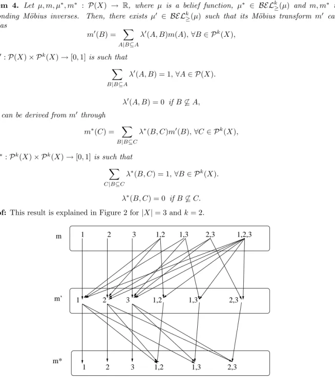
Theorem 4. Let µ, m, µ∗, m∗ : P(X) → R, where µ is a belief function, µ∗ ∈ BELk
≥(µ) and m, m∗ their
corresponding M¨obius inverses. Then, there exists µ′ ∈ BELk
≥(µ) such that its M¨obius transform m′ can be
written as
m′(B) = X
A|B⊆A
λ′(A, B)m(A), ∀B ∈ Pk(X),
where λ′ : P(X) × Pk(X) → [0, 1] is such that
X
B|B⊆A
λ′(A, B) = 1, ∀A ∈ P(X). (5)
λ′(A, B) = 0 if B 6⊆ A, (6) and m∗ can be derived from m′ through
m∗(C) = X
B|B⊆C
λ∗(B, C)m′(B), ∀C ∈ Pk(X), (7)
where λ∗: Pk(X) × Pk(X) → [0, 1] is such that
X
C|B⊆C
λ∗(B, C) = 1, ∀B ∈ Pk(X). (8)
λ∗(B, C) = 0 if B 6⊆ C. (9) Proof: This result is explained in Figure 2 for |X| = 3 and k = 2.
1 2 3 1,2 1,3 2,3 1,2,3 1 2 3 1,2 1,3 2,3 1 2 3 1,2 1,3 2,3 m m’ m*
Figure 2: Example of flow network for n = 3 and k=2. We already know from Theorem 3 that
m∗(C) = X
A|C∩A6=∅
λ(A, C)m(A), λ(A, C) ≥ 0, X
A|A∩C6=∅
λ(A, C) = 1, ∀A ∈ P(X), ∀C ∈ Pk(X).
Let us define a weight function λ′ by
λ′(A, B) := X
C|C∩A=B
Then, we define m′ by
m′(B) := X
A|B⊆A
λ′(A, B)m(A), ∀B ∈ Pk(X). (11)
Let us check that λ′ satisfies the conditions imposed in the theorem.
• λ′(A, B) = X
C|C∩A=B
λ(A, C) ≥ 0, ∀A ∈ P(X), ∀B ∈ Pk(X), as λ(A, C) ≥ 0, ∀A ∈ P(X), ∀C ∈ Pk(X) by
Theorem 3. • X B|B⊆A λ′(A, B) = X B|B⊆A X C|C∩A=B λ(A, C) = X C|C∩A6=∅
λ(A, C) = 1, ∀A ∈ P(X) by Theorem 3, so that Equa-tion (5) holds.
• Equation (6) is satisfied by the construction of λ′.
• Let us now prove that µ′ is a belief function: First,
m′(B) = X
A|B⊆A
λ′(A, B)m(A) ≥ 0, ∀B ∈ Pk(X)
because µ is a belief function (and then m(A) ≥ 0, ∀A ⊆ X by Proposition 2), and λ′(A, B) ≥ 0, ∀A ∈
P(X), ∀B ∈ Pk(X).
Then, it suffices to prove that X
B⊆X
m′(B) = 1, but this holds since
X B∈Pk(X) m′(B) = X B⊆X X A|B⊆A λ′(A, B)m(A) = X A⊆X X B|B⊆A λ′(A, B)m(A) = X A⊆X m(A) = 1. • Besides, µ′ dominates µ: µ′(B) = X D⊆B m′(D) = X D⊆B X A|D⊆A λ′(A, D)m(A).
If A ⊆ B, we have that whenever D ⊆ A, then D ⊆ B, and hence, m(A) is multiplied by X D|D⊆A λ′(A, D) = 1. Consequently, X D⊆B m′(D) = X A⊆B m(A) + X A6⊆B X D|A∩B=D λ′(A, D)m(A).
Finally, as m(A) ≥ 0, ∀A ∈ P(X), λ′(A, B) ≥ 0, ∀A ∈ P(X), ∀B ∈ Pk(X), we obtain that
µ′(B) ≥ X
A⊆B
m(A) = µ(B).
• µ′ generates µ∗ through Equation (7): For each B, C such that B ⊆ C let us define
λ∗(B, C) := X
A|A∩C=B
λ(A, C)m(A) m′(B), if m
′(B) 6= 0.
What happens if m′(B) = 0? In this case, for all A such that B ⊆ A, we have λ′(A, B) = 0 or m(A) = 0
by Equation (11) and thus, λ(A, C) = 0, or m(A) = 0, ∀C such that A ∩ C = B by Equation (10). We can then choose arbitrary values for λ∗(B, C) under the conditions of Equations (8) and (9).
Then, X B⊆C λ∗(B, C)m′(B) = X B⊆C X A|A∩C=B λ(A, C)m(A) m′(B)m ′(B) = X B⊆C X A|A∩C=B λ(A, C)m(A) = X A|A∩C6=∅ λ(A, C)m(A) = m∗(C),
by Theorem 3. Thus, with our definitions of µ′ and λ∗, we have obtained µ∗.
It is clear that λ∗(B, C) ≥ 0, ∀B, C ∈ Pk(X) as λ(A, C) ≥ 0, m(A) ≥ 0, m′(B) ≥ 0, ∀A ∈ P(X), ∀B ∈
Pk(X).
To finish the proof, it suffices to show that for any B ∈ Pk(X), we have X
C|B⊆C λ∗(B, C) = 1. We have X C|B⊆C λ∗(B, C) = X C|B⊆C X A|A∩C=B λ(A, C)m(A) m′(B)= 1 m′(B) X A,C|C∩A=B λ(A, C)m(A) = 1 m′(B) X A⊆X|B⊆A X C∈Pk(X)|C∩A=B λ(A, C)m(A) = 1 m′(B) X A⊆X|B⊆A λ′(A, B)m(A) = 1 m′(B)m ′(B) = 1.
Then, the result holds.
As a final remark, note that we can find some examples where we can ensure λ ≥ 0, even if µ is not a belief function:
Example 5. Consider |X| = 4 and the capacity defined by µ(A) = 1, if A 6= ∅ (this is u∅, which is not a belief
function by Proposition 2). Then, the only n-additive capacity that dominates µ is µ itself. Then, function λ that determines the only capacity dominating µ (i.e. µ) is given by λ(A, A) = 1, λ(A, B) = 0 if A 6= B, and thus λ is a non-negative function, even if µ is not a belief function.
5
Application to decision making
We illustrate in this section several possible applications of the above results, i.e., the construction of the set of k-additive belief functions dominating a given capacity.
A whole set of applications comes from the following situation: suppose that we want to build a decision model from some elicitation procedure with a human decision maker. Most of the time, the decision maker is not able to provide enough information or enough precise answers in order to have a unique possible decision model compatible with the information obtained from the decision maker. In our case, we make the assumption that our decision model is based on capacities, which is known in many fields of decision making to provide versatile models. This means that the parameters of our model are precisely the coefficients of a capacity µ, and that we cannot expect better information than µ(A) belongs to some interval [µ∗(A), µ∗(A)], for all subset A of the
referential set X.
Let us first consider the lower bound µ∗, since in many cases the upper bound may be simply the uninformative
value 1. Depending on the specific domain of application and type of decision problem, one may want to restrict to some particular family of capacities, say F, so that the problem of identification of the decision model writes: find all capacities in F dominating µ∗. The choice of a particular family of capacities is principally based on two
reasons:
• we are looking for capacities satisfying a given set of properties, most often properties linked to decision behaviour (attitude towards risk, etc.). This is related to the axiomatic approach to decision making.
• to limit the number of possible solutions and to limit complexity of the model, we impose some restrictions, typically, k-additivity.
The case of k-additive belief functions appear as a natural choice for F at least in the following cases:
• in social welfare theory, the case of k-additive belief functions has been characterized by the authors [22], following previous works of Ben Porath and Gilboa [23], and Gajdos [7], with axioms which are natural in the context of social welfare since they are closely related to the well-known Gini index. In particular, it is proved that k-additivity can be seen as an aversion to social inequality.
• in decision under uncertainty or risk, the meaning of a belief function, compared to a classical probability measure, is well known. Roughly speaking, belief functions permit to distinguish between ignorance and equiprobability, a feature which is particularly useful for handling missing or ambiguous data. There also exist various axiomatic characterization results of belief functions, see e.g. Jaffray and Wakker [14], and Wakker [29].
For example, assume |X| = 3 and suppose that from the information given by the decision maker, we can only deduce that µ∗(3) ≥ 0.4 and µ∗(A) ∈ [0, 1] for A 6= {3}. Then, the lower measure is a belief function given by
m∗(3) = 0.4, m∗(X) = 0.6, m∗(A) = 0, otherwise.
Then, the set of all 2-additive belief measures compatible with the information is given by the set of dominant belief functions in MΛ2
∩,+(µ) by Theorem 3, and these measures can be generated from MΛ 2
⊆,+(µ) by Theorem 4.
In order to be complete, the upper bound should be considered as well, which motivates a companion study for the set of k-additive belief functions dominated by some capacity.
A second possible application arises in cooperative game theory, where X represents the set of players. The notion of dominating probability measure (in fact additive non normalized capacities since in this context µ(X) represents the total worth of the game, which in general is not equal to 1) is known in this domain under the name of “core of a game”. The existence of the core is closely related to the formation of coalitions, since any additive (non normalized) capacity in the core represents a distribution of some non negative amount to each player. Defining the core as the set of dominating k-additive belief functions generalizes the classical definition in the sense that the distribution will be defined over individual players and all coalitions of at most k players. The fact that we impose belief functions guarantees that the amount will be non negative, since it corresponds to the M¨obius transform.
In all cases, the notion of k-additive belief function appears as the most natural generalization of probability measures, the value of k measuring the complexity of the generalization. In this finite setting, a probability measure is defined by its probability distribution over all singletons, which is a non-negative amount. A 2-additive belief function induces a non negative distribution over singletons and pairs, and so on.
6
Conclusions and open problems
In this paper we have studied the set of k-additive belief functions dominating a given capacity. This set is a middle term between the set of dominating probabilities and the set of dominating k-additive measures.
We have seen that the results for the general k-additive case do not allow a translation of the results derived for probabilities in [1]. This is due to the fact that the conditions are too general, thus leading a too wide set of functions.
We have obtained a result, similar to those for dominating probabilities and k-additive measures, that gives us a family of functions in which the set of dominating k-additive belief functions is included. Our results for belief functions permit a reduction in the set of functions. However, the family obtained in this case is not the natural extension of the corresponding family obtained for probabilities and provides again a too wide set of functions.
Finally, we have proved that it suffices to consider this natural extension in order to derive any other dominating k-additive belief function whenever the initial measure is a belief function, too.
We have proposed several possible applications in decision making, especially in social welfare and decision under risk or uncertainty.
As immediate research, we have the problem of finding the profile of BELk≥(µ) when µ is a 2-monotone measure or a belief function. In this sense, we have already found some results in [21], where Theorem 4 plays an important role.
Another interesting problem is to look for extensions of Theorem 4. Finally, two other questions arise from a theoretical point of view:
1. We have proved that for belief functions, λ ≥ 0. However, this is not a necessary condition (Example 5). Then, we can ask ourselves for necessary and sufficent conditions on µ for λ ≥ 0.
2. The same problem can be considered for the A ⊆ B condition.
7
Acknowledgements
This research has been supported in part by FEDER-MCYT grant number BFM2001-3515.
References
[1] A. Chateauneuf and J.-Y. Jaffray. Some characterizations of lower probabilities and other monotone capacities through the use of M¨obius inversion. Mathematical Social Sciences, (17):263–283, 1989.
[2] G. Choquet. Theory of capacities. Annales de l’Institut Fourier, (5):131–295, 1953.
[3] A. P. Dempster. Upper and lower probabilities induced by a multivalued mapping. The Annals of Mathematical Statististics, (38):325–339, 1967.
[4] D. Denneberg. Non-additive measures and integral. Kluwer Academic, 1994.
[5] D. Denneberg. Non-additive measure and integral, basic concepts and their role for applications. In T. Murofushi M. Grabisch and M. Sugeno, editors, Fuzzy measures and integrals. Theory and applications, volume 40 of Studies in Fuzziness and Soft Computing, pages 42–69. Physica-Verlag, 2000.
[6] D. Dubois and H. Prade. A class of fuzzy measures based on triangular norms. Int. J. General Systems, 8:43–61, 1982.
[7] T. Gajdos. Measuring inequalities without linearity in envy: Choquet integral for symmetric capacities. Journal of Economic Theory, 106:190–200, 2002.
[8] D. Gale. The Theory of Linear Economic Models. Mc Graw Hill, New York, 1960.
[9] M. Grabisch. k-order additive discrete fuzzy measures. In Proceedings of 6th International Conference on Information Processing and Management of Uncertainty in Knowledge-Based Systems (IPMU), pages 1345–1350, Granada (Spain), 1996.
[10] M. Grabisch. k-order additive discrete fuzzy measures and their representation. Fuzzy Sets and Systems, (92):167–189, 1997.
[11] M. Grabisch. Upper approximation of non-additive measures by k-additive measures- The case of belief functions. In Proceedings of 1st International Symposium on Imprecise Probabilities and Their Applications (ISIPTA), Ghent (Belgium), June 1999.
[12] M. Grabisch. The interaction and M¨obius representations of fuzzy measures on finite spaces, k-additive measures: a survey. In M. Grabisch, T. Murofushi, and M. Sugeno, editors, Fuzzy Measures and Integrals- Theory and Applications, number 40 in Studies in Fuzziness and Soft Computing, pages 70–93. Physica–Verlag, 2000.
[13] M. Grabisch. On lower and upper approximation of fuzzy measures by k-order additive measures. In B. Bouchon-Meunier, R. R. Yager, and L. Zadeh, editors, Information, Uncertainty, Fusion, pages 105–118. Kluwer Sci. Publ., 2000. Selected papers from IPMU’98.
[14] J.-Y. Jaffray and P. Wakker. Decision making with belief functions: Compatibility and incompatibility with the sure-thing principle. Journal of Risk and Uncertainty, 7:255–271, 1993.
[15] J.-L. Marichal. k-intolerant capacities and Choquet integrals. European Journal of operational Research, to appear. [16] P. Miranda and M. Grabisch. Optimization issues for fuzzy measures. International Journal of Uncertainty, Fuzziness
[17] P. Miranda and M. Grabisch. Characterizing k-additive fuzzy measures. In Proceedings of Eighth International Conference of Information Processing and Management of Uncertainty in Knowledge-based Systems (IPMU), pages 1063–1070, Madrid (Spain), July 2000.
[18] P. Miranda and M. Grabisch. p-symmetric fuzzy measures. In Proceedings of Ninth International Conference of Information Processing and Management of Uncertainty in Knowledge-based Systems (IPMU), pages 545–552, Annecy (France), July 2002.
[19] P. Miranda, M. Grabisch, and P. Gil. Dominance of fuzzy measures by k-additive belief functions. In Int. Fuzzy Systems Association World Congress (IFSA 2003), pages 143–146, Istanbul, Turkey, June 2003.
[20] P. Miranda, M. Grabisch, and P. Gil. Identification of non-additive measures from sample data. In R. Kruse G. Della Riccia, D. Dubois and H.-J. Lenz, editors, Planning based on Decision Theory, volume 472 of CISM Courses and Lectures, pages 43–63. Springer Verlag, 2003.
[21] P. Miranda, M. Grabisch, and P. Gil. On some results of the set of dominating k-additive belief functions. In Pro-ceedings of Tenth International Conference on Information Processing and Management of Uncertainty in Knowledge-Based Systems, pages 625–632, Perugia (Italy), 2004.
[22] P. Miranda, M. Grabisch, and P. Gil. Axiomatic structure of k-additive capacities. Mathematical Social Sciences, 49:153–178, 2005.
[23] E. Ben Porath and I. Gilboa. Linear measures, the Gini index, and the income-equality trade-off. Journal of Economic Theory, (64):443–467, 1994.
[24] G. C. Rota. On the foundations of combinatorial theory I. Theory of M¨obius functions. Zeitschrift f¨ur Wahrschein-lichkeitstheorie und Verwandte Gebiete, (2):340–368, 1964.
[25] G. Shafer. A Mathematical Theory of Evidence. Princeton University Press, Princeton, New Jersey, (USA), 1976. [26] L. S. Shapley. Cores of convex games. International Journal of Game Theory, 1:11–26, 1971.
[27] M. Sugeno. Theory of fuzzy integrals and its applications. PhD thesis, Tokyo Institute of Technology, 1974. [28] M. Sugeno and T. Terano. A model of learning based on fuzzy information. Kybernetes, (6):157–166, 1977.
[29] P. Wakker. Dempster belief functions are based on the principle of complete ignorance. Int. J. of Uncertainty, Fuzziness and Knowledge-Based Systems, 8:271–284, 2000.
[30] P. Walley. Coherent lower (and upper) probabilities. Technical Report 22, U. of Warwick, Coventry, (UK), 1981. [31] P. Walley and T. L. Fine. Towards a frequentist theory of upper and lower probability. Ann. of Stat., 10:741–761,
1982.
[32] M. Wolfenson and T. L. Fine. Bayes-like decision making with upper and lower probabilities. J. Amer. Statis. Assoc., (77):80–88, 1982.