HAL Id: lirmm-01381088
https://hal-lirmm.ccsd.cnrs.fr/lirmm-01381088
Submitted on 1 Nov 2019
HAL is a multi-disciplinary open access
archive for the deposit and dissemination of
sci-entific research documents, whether they are
pub-lished or not. The documents may come from
teaching and research institutions in France or
abroad, or from public or private research centers.
L’archive ouverte pluridisciplinaire HAL, est
destinée au dépôt et à la diffusion de documents
scientifiques de niveau recherche, publiés ou non,
émanant des établissements d’enseignement et de
recherche français ou étrangers, des laboratoires
publics ou privés.
Mining Epidemiological Dengue Fever Data from Brazil:
A Gradual Pattern Based Geographical Information
System
Yogi Satrya Aryadinata, Yuan Lin, Christovam Barcellos, Anne Laurent,
Thérèse Libourel Rouge
To cite this version:
Yogi Satrya Aryadinata, Yuan Lin, Christovam Barcellos, Anne Laurent, Thérèse Libourel Rouge.
Mining Epidemiological Dengue Fever Data from Brazil: A Gradual Pattern Based Geographical
Information System. 15th International Conference on Information Processing and Management of
Uncertainty in Knowledge-Based Systems (IPMU), LIRMM, Jul 2014, Montpellier, France.
pp.414-423, �10.1007/978-3-319-08855-6_42�. �lirmm-01381088�
Mining epidemiological Dengue Fever Data from Brazil:
a gradual pattern based geographical information
system
Y. Aryadinata∗, Y. Lin∗∗, C. Barcellos∗∗∗, A.Laurent∗, and T.Libourel∗∗ ∗LIRMM, Montpellier, France
{aryadinata,laurent}@lirmm.fr ∗∗UMR ESPACE-DEV (IRD-UM2), Montpellier, France, [email protected],[email protected]
∗∗∗Funda´c˜o Oswaldo Cruz, Rio de Janeiro, Brazil [email protected]
Abstract. Dengue fever is the world’s fastest growing vector-borne disease. Study-ing such data aims at better understandStudy-ing the behaviour of this disease to prevent the dengue propagation. For instance, it may be the case that the number of cases of dengue fever in cities depends on many factors, such as climate conditions, density, sanitary conditions. Experts are interested in using geographical infor-mation systems in order to visualize knowledge on maps. For this purpose, we propose to build maps based on gradual patterns. Such maps provide a solution for visualizing for instance the cities that follow or not gradual patterns. Keywords: Epidemiological Data, Data Mining, Geographic Information Sys-tems, Gradual Patterns.
1
Introduction
There are approximately 50 millions new cases each year, and approximately 2.5 billion people live in endemic countries [1] located in the tropical zone between the lati-tudes of 35◦N and 35◦[2]. The vector for dengue infection is Aedes aegypti, which has a strictly synanthropic lifestyle [3]. The proliferation of these mosquitoes is supported by both weather patterns and the contemporary style of human life in large cities, where large amounts of water are deposited in the environment and become potential breeding grounds for mosquito reproduction [4]. These factors have been shown to influence the occurrence and spread of dengue infection over the last 50 years.
The incidence of dengue infection has a characteristic seasonal movement in al-most all regions of the world, where periods of high transmissibility are experienced during certain months of the year. This phenomenon has been explained by the close relationship between the density variation in winged forms of the vector and climatic conditions [5, 6], such as rainfall, temperature and relative humidity.
Since 1986, Brazil has been affected by dengue epidemics that have reached dra-matic proportions. This country of continental dimensions has a wide territorial range of
tropical and subtropical climates (hot and humid), with an average annual temperature above 20◦C and rainfall exceeding 1,000 mm per year. These characteristics provide suitable abiotic conditions for the survival of Aedes aegypti [7], the main dengue vector present in the Americas.
From 1990 to 2010, 5.98 million cases of dengue were reported, and autochthonous cases have been recorded in 80% of the 5,565 Brazilian municipalities. The period of greatest risk for dengue occurrence has been shown to be during or immediately follow-ing the rainy season [5,6], and there is a reduced incidence durfollow-ing the remainfollow-ing months of the year. However, epidemiological studies on the relationship between dengue infec-tion and climate variables in Brazil are scarce.
Studies in wide (national) geographical scales and considering the interactions be-tween spatial and time are still scarce in dengue literature. [3] revealed rapid travelling waves of DHF crossing Thailand emanating from Bangkok every 3 years. Inversely, in Cambodia seasonal propagation waves are originated in poor rural areas being their propagation conditioned by road traffic [8]. In Peru, dengue spatial and temporal dy-namics was influenced by the different sociodemographic and environmental among eco-regions [9]. The recent spread of dengue in Brazil is equally related to human mo-bility across cities network and leaving remote country regions relatively protected [10]. However, unlike contagious diseases, dengue transmission is constrained the environ-mental substrate on which vector must reproduce and infect people. Thus, the presence and abundance of vector are necessary but not sufficient condition to dengue transmis-sion.
Climate and environmental changes may exacerbate the present distribution of vec-tor borne diseases as well as extend transmission to new niches and populations [11]. Both trends underline the role of health surveillance systems in order to detect and conduct preventive actions in unusual transmission contexts. Climate changes affect populations in different ways and intensities according to the vulnerability of social groups, which is associated to their insertion in place and society. Spatial analysis offers important tools to describe measure and monitor health impact on vulnerable popula-tions under possible scenarios. Brazilian territory presents a wide variety of temperature ranges and rainfall regimes. In addition to climatic variations, unequal urban infrastruc-ture among cities and differential territory occupation patterns increases the complexity of dengue nationwide dynamics.
The important questions arising from experts debate and studies are :
1. Which patterns were more important to explain dengue distribution? What is im-portant? Climate? Sanitary conditions? Human mobility?
2. Which years are typical and regular (the same patterns appear along all years)? And which are abnormal (patterns are different for one atypical year)? For example, extreme climate events, el Ni˜no ?
3. Mapping the patterns. Are patterns concentrated (spatial clusters)? Where are lo-cated the different (and contradictory) patterns?
4. Is this spatial pattern related to other geographical features? (relief, ecosystems, roads, rivers, urban regions, etc.).
In this paper, we propose a method using a gradual pattern mining to analyze and to discover the patterns of behavior in dengue fever cases in Brazil. This method also
Gradual Maps 3 allows us to produce a gradual map that can directly be used to see the behavior of the cases of dengue fever from the geographic approach.
In Section 2, we introduce the method to find the gradual patterns, which can be used to create binary and gradual map that described in Section 3. Section 4 presents the data and indicators in terms of analysis and how to produce the binary map (Section 4.2) and the gradual map (Section 4.3). Section 5 concludes the paper and gives the perspectives of our research.
2
Gradual Patterns
Gradual pattern mining has been recently introduced as the topic addressing the automatic discovery of gradual patterns from large databases. Such databases are struc-tured over several attributes which domains are totally ordered, considering a relation ≤. For instance Table 1 reports an example of such a database.
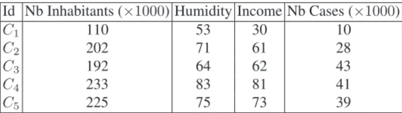
We consider a toy database containing the information about a disease taken on five cities. Each tuple from the table 1 corresponds to a city, and reports the number of cases for this disease (last column) studied by respect with the number of inhabitants from the city (in thousands), the average humidity (in percentage), and the average income (in K euros).
Table 1. Database D describing a toy example for a disease in 5 cities Id Nb Inhabitants (×1000) Humidity Income Nb Cases (×1000)
C1 110 53 30 10
C2 202 71 61 28
C3 192 64 62 43
C4 233 83 81 41
C5 225 75 73 39
An example of gradual patterns is The higher the number of inhabitants, the higher
the degree of Humidity, the higher the number of cases of the disease.
We remind below some concepts of the literature on gradual patterns.
Definition 1. Gradual item. A gradual item is a pair (i, v) where i is an item and v is variation v ∈ {↑, ↓}. ↑ stands for an increasing variation while ↓ stands for a
decreasing variation.
Example 1. (N bInhabitants, ↑) is an item of graduel item.
Definition 2. Gradual Pattern (also known as Gradual Itemset). A gradual pattern is a
set of gradual items, denoted by GP = {(i1, v1), . . . , (in, vn)}. The set of all gradual
patterns that can be defined is denoted by GP.
Example 2. {(N bInhabitants, ↑), (Humidity, ↑), (N bCases, ↑)} is a gradual
Gradual pattern mining aims at extracting the frequent patterns, as in the classical data mining framework for itemsets and association rules.
Definition 3. Given a threshold of a minimum support σ, a gradual pattern GP is said
to be frequent if supp(GP ) ≥ σ.
For describing what frequent means in the context of gradual patterns, several sup-ports have been proposed in the literature. All these materials are based on the idea that it takes the number / proportion of transactions in the database (e.g., the number / proportion of cities in our example) that respect the pattern. For being counted, a trans-action must behave adequately with respect to other cities. For example, in Table 2, we see that the number of cases and the number of inhabitants increase together for cities 1 and 2, as 110 < 202 and 10 < 28. If the variation is decreasing (↓) then the num-bers must follow it. For instance for cities3 and 4, the number of inhabitants increases ((Inhabitants, ↑)) and the number of cases ((cases, ↓)) decreases as 192 < 233 and 43 > 41.
One of the support proposed in the literature [12] is based on the length of the longest path of cities that can be built using this idea.
Definition 4. The support of gradual pattern GP is given by the following formula : support(GP ) =maxL∈l(|L|)
(|R|) .
For determining the longest path, we build the precedence graph for the pattern being considered (Fig. 1). It can be the case that several paths can be built for a pat-tern, as shown below when trying to order the cities with respect with the pattern {(N bInhabitants, ↑), (Humidity, ↑), (N bCases, ↑)}. Two orderings are possible: L1 and L2.
Table 2. Two list obtained of{(N bInhabitants, ↑), (Humidity, ↑), (N bCases, ↑)} : L1 and L2 (from left to right)
Id Nb Inhabitants Humidity Nb Cases
C1 110 53 10
C2 202 71 28
C4 233 83 41
Id Nb Inhabitants Humidity Nb Cases
C1 110 53 10
C2 202 71 28
C5 225 75 39
Precedence graphs can also be represented in the form of binary matrices as shown in Table 3 for the pattern {(N bInhabitants, ↑), (Humidity, ↑), (N bCases, ↑)}. C2
precedes C4and C5(value 1 of the matrix), but not C1and C3(value 0 of the matrix).
We have here: support ({(N bInhabitants, ↑), (Humidity, ↑), (N bCases, ↑)}) =3 5as
P is taken by the maximum list of cities < C1, C2, C4> and < C1, C2, C5> .
For representing a pattern on the whole database, we consider precedence graphs, as shown by Fig. for the pattern{(N bInhabitants, ↑), (Humidity, ↑), (N bCases, ↑ )}. Such a graph can be represented in a binary matrix, which allows to optimize the computations. For instance, there are two longest paths in this example: < C1, C2, C4>
Gradual Maps 5 C1 C2 C4 C3 C5
Fig. 1. Precedence graph associated to the pattern {(N bInhabitants, ↑), (Humidity, ↑ ), (N bCases, ↑)}
Table 3. Binary matrix associated to the pattern {(N bInhabitants, ↑), (Humidity, ↑ ), (N bCases, ↑)} City C1C2C3C4 C5 C1 1 1 1 1 1 C2 0 1 0 1 1 C3 0 0 1 0 0 C4 0 0 0 1 0 C5 0 0 0 0 1
In our work, we aim at displaying such gradual patterns computing from geograph-ical data on maps. For this purpose, we propose to display cities in a form (e.g., color or size) that depends on whether it contributes or not to some gradual pattern. For instance, if the city 1 does not behave the same as all the other cities for pattern (Humidity, ↑), (N bCases, ↑) then it will be pointed out be being displayed in red
why all the other cities will be colored in green.
3
Building Binary and Gradual Maps
In this section, we present novel methods for visualizing gradual patterns on maps. We propose two methods of visualization. Both these methods rely on the calculation of the support with the longest path in the precedence graph
Our idea is to produce maps starting from the extraction of gradual patterns. We will explain this part with a simple example of a region that contains five cities(C1, C2, C3
,-C4, C5). Based on data from these cities, we believe we have an interesting pattern that
we can apply in a map. We then want to know, for each city, how it contributes or not to identify spatial pattern. Then we can represent this information to the user on the maps which he is accustomed. The principle is that each pattern corresponds to a layer in the GIS. Cities are then represented differently depending on their contribution to the cause, i.e., a dichotomous variable.
Table 4. The list of longest paths associated to Fig. 1 List Length
C1, C3 2
C1, C2, C4 3
C1, C2, C5 3
We consider two approaches. The first approach, called ”binary map” is to represent a color (e.g., green) the cities that contribute to maximum path length on the pattern, and within another color (e.g. red) other cities. The second approach is to represent the intensity of the color cities that are in the longest path and less intense color for cities that are in the shortest path. This is called ”gradual map”, i.e., a continuous variable.
3.1 Binary Map
In this binary map, we identify items through its participation in the gradual pattern (between 0 and 1) we use the following steps:
1. Calculating each item of the support in line with the binary matrix 2. Extract lines that have the maximum support
3. Identification (green (1)) cities that are included in the set of itemset length of the maximum path.
4. Identification (red (0)) of the cities that are not in the set of itemset length of the maximum path.
By looking at Figure 1, we know the cities which respect the gradual interesting pattern. For example, Figure 2 shows that the city C5 is red, do not fully respect the
gradual pattern. In contrast, other cities are green because they are in the longest path
Yes No C1 C4 C5 C2 C3
Fig. 2. Binary Map
Minimum Support C1 C3 C4 C5 C2
Gradual Maps 7 3.2 Gradual Map
In order to realize a more detailed maps of the binary map. To do this, we propose a gradual map to visualize the value of the support of each item which corresponds to a proportion of belonging to a support item. To realize this map, we consider the following steps:
1. Calculate the support of each item per line in the binary matrix 2. Take the maximal support size
3. Calculate the intensity of each item in order to identify the importance of which item depends on its intensity value
Intensity(v) = T he length of support of vT he maximum path length
4. From the intensity value make the classification using the color indicator on the map.
With this map, we can identify the cities that are more important than others con-cerning the classification defined in the figure. Thus, the city be more or less illuminated depending on the length of the maximum path in which it appears. For example, in Fig-ure 3, the cities C1, C3 and C4 are the most illuminated because they belong to the
maximum path length.
4
Experimentation
Therefore, in our experimentation we use our methods with the dengue cases in Brazil. Firstly, we analyse the data sources and indicators that described in Section 4.1 and Section 4.2 and 4.3 to build the binary and gradual maps.
4.1 Data sources and Indicators
Dengue fever (DF) notifications from 2001 to 2012 were summarized by year of symptoms upset and municipality of residence. Data were obtained from the Notifi-able Diseases Information System (SINAN acronym in Portuguese), organized by the Brazilian Ministry of Health and freely available in Health Information Department (Datasus). Cases are defined as confirmed Dengue Fever (DF) or Dengue Hemorrhagic Fever (DHF). Cases are confirmed by clinical and laboratory according to standard procedures and submitted to epidemiological investigation by local health surveillance teams. Approximately 30% of the cases of dengue are also laboratory-confirmed.
The socio-demographic data were obtained from the website of the Brazilian Insti-tute of Geography and Statistics (Instituto Brasileiro de Geografia e Estatstica IBGE; http://mapas.ibge.gov.br). Cities were categorized according to the climate classifica-tion map of climate obtained from the Brazilian Institute of Geography and Statistics (IBGE). There are four types of variables on this data: Temperature regime was classi-fied in three categories, Rainfall regime was categorized into four classes, Humidity was categorized into four classes, Sanitary conditions were summarized by the combination of three variables, Mobility was evaluated by means of two variables.
Individual variables were ranked and the result of summing the ranks was used to categorize into four classes: Very high, High, Medium and Low. All indicators were geocoded and mapped using the coordinates of the city as the center of gravity on the common 5506 existing in 2010. This position was used to create maps and assign information from other layers, such as climate, in a geographic information system (GIS).
During the extraction process of gradual patterns, we cleaned the data so that they do not contain any missing values, false values, etc. In Section 2, we introduced methods for research on dengue epidemic. Then, we will apply these methods in order to obtain better results.
For simplicity, we choose 25 towns in the state of Rio de Janeiro, Brazil. The State of Rio de Janeiro (RJ) is located east of the southeast region. The capital is Rio de Janeiro. This state has an area of 43 909 km2with about 14,367,000 mainly concentrated along the coast. We choose the state of Rio de Janeiro because of the high frequency of dengue outbreaks in the region. In addition, this region presents a wide morphological diversity (mountains, beaches, dunes, lagoons, etc..). In general, it is divided into three major geographical subregions: the metropolitan lowlands (often called Baixada Fluminense), coastal elevations and northern lowlands. The climate is tropical and the average annual temperature is 23◦C. With this data, we extract the gradual patterns with the method of extraction of conventional gradual patterns on the Section 2.
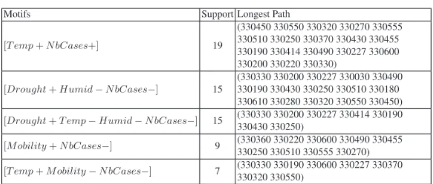
Table 5 displays some of the interesting gradual patterns in the case of epidemic dengue. After looking at the Table 5 and patterns found, we can infer that the climate (the drought, temperature, humidity) plays the most important role in the case of the dengue epidemic, followed by the level of mobility and sanitation state level.
Table 5. Example of extracted gradual patterns (Support = 0.25)
Motifs Support Longest Path
[T emp + N bCases+] 19
(330450 330550 330320 330270 330555 330510 330250 330370 330430 330455 330190 330414 330490 330227 330600 330200 330220 330330)
[Drought + Humid − N bCases−] 15
(330330 330200 330227 330030 330490 330190 330430 330250 330510 330180 330610 330280 330320 330550 330450) [Drought + T emp − Humid − N bCases−] 15 (330330 330200 330227 330414 330190
330430 330250)
[M obility + N bCases−] 9 (330360 330220 330600 330490 330455 330250 330510 330555 330270) [T emp + M obility − N bCases−] 7 (330330 330190 330600 330227 330370
330320 330550)
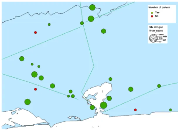
Finally, we can make a binary map and a gradual map that take into account the gradual patterns on the dengue epidemic in Brazil in Fig. 4 and Fig. 5 for the pattern [T emp + M obility − N bCases−].
Gradual Maps 9 4.2 Binary Map
Fig. 4 shows the majority of the cities, following the pattern(T emperature, ↑ ), (M obility, ↓), (N bCases, ↓), displayed in green.
Nb. dengue fever cases Member of pattern
Yes No
Fig. 4. Binary Map (T emperature,↑), (M obility, ↓), (N bCases, ↓)
4.3 Gradual Map
In Fig. 5, we present the support level(0 − 1) of the cities using the intensity color. This map shows more detail information than binary map,Which cities are more related to the pattern(T emperature, ↑), (M obility, ↓), (N bCases, ↓). We can see that impor-tant emerging epidemic dengue fever mostly appeared in cities located around the coast (shown with the green intensity).
The difficulty of this step is the production of maps from found gradual patterns, but it is important to retrieve all the items in each pattern corresponding to the length of maximum path.
5
Conclusion
In this article, we study how gradual patterns can help to produce maps in geograph-ical information systems. We apply our method in the context of dengue epidemics in Brazil.
Our main perspectives are to merge more criteria for building such maps and to study how a large volume of gradual maps can be displayed to end-users in a user-friendly way by using the so-called layers in geographical information system tools.
References
1. Organization, W.H.: [The world health report 2006: working together for health]. (2006) 2. Gubler, D., Ooi, E., Vasudevan, S., Farrar, J.: Dengue and Dengue Hemorrhagic Fever. CABI
(2013)
3. Gubler, D.J.: Dengue, urbanization and globalization: The unholy trinity of the 21st century (2011)
4. Kovats, R., Campbell-Lendrum, D., McMichael, A., Woodward, A., Cox, J.: Early effects of climate change: do they include changes in vector-borne disease? Philos Trans R Soc Lond B Biol Sci 356(1411) (2001) 1057–68
5. Souza-Santos, R.: [the factors associated with the occurrence of immature forms of aedes aegypti in ilha do governador, rio de janeiro, brazil]. Rev Soc Bras Med Trop 32(4) 6. Souza-Santos, R., Carvalho, M.: [spatial analysis of aedes aegypti larval distribution in the
ilha do governador neighborhood of rio de janeiro, brazil]. Cad Saude Publica 16(1) 7. Yang, H.M., Macoris, M.L., Galvani, K.C., Andrighetti, M.T., Wanderley, D.M.: Dinˆamica
da transmissao da dengue com dados entomol´ogicos temperatura-dependentes. Tema–Tend. Mat. Apl. Comput 8(1) (2007) 159
8. Teurlai, M., Huy, R., Cazelles, B., Duboz, R., Baehr, C., Vong, S.: Can human movements explain heterogeneous propagation of dengue fever in cambodia? PLoS Negl Trop Dis 6(12) (12 2012) e1957
9. Chowell, G., Cazelles, B., Broutin, H., Munayco, C.V.: The influence of geographic and climate factors on the timing of dengue epidemics in Peru, 1994-2008. Bmc Infectious Diseases 11 (2011) p. 164
10. Cat˜ao, R.d.C., Guimar˜aes, R.B.: Mapeamento da reemergˆencia do dengue no brasil–1981/82-2008. Hygeia 7(13) (2011)
11. McMichael, A., Lindgren, E.: Climate change: present and future risks to health, and neces-sary responses. J Intern Med 270(5) (2011) 401–13
12. Di-Jorio, L., Laurent, A., Teisseire, M.: Mining frequent gradual itemsets from large databases. In: Proc. of the 8th Int. Symposium on Intelligent Data Analysis