Automatic Self-Calibration of Suspended Under-Actuated Cable-Driven Parallel Robot using Incremental Measurements

HAL Id: hal-02430605

https://hal.inria.fr/hal-02430605

Submitted on 7 Jan 2020

HAL is a multi-disciplinary open access

archive for the deposit and dissemination of

sci-entific research documents, whether they are

pub-lished or not. The documents may come from

teaching and research institutions in France or

abroad, or from public or private research centers.

L’archive ouverte pluridisciplinaire HAL, est

destinée au dépôt et à la diffusion de documents

scientifiques de niveau recherche, publiés ou non,

émanant des établissements d’enseignement et de

recherche français ou étrangers, des laboratoires

publics ou privés.

Automatic Self-Calibration of Suspended

Under-Actuated Cable-Driven Parallel Robot using

Incremental Measurements

Edoardo Idá, Jean-Pierre Merlet, Marco Carricato

To cite this version:

Edoardo Idá, Jean-Pierre Merlet, Marco Carricato. Automatic Self-Calibration of Suspended

Under-Actuated Cable-Driven Parallel Robot using Incremental Measurements. CableCon 2019 - 4th

Inter-national Conference on Cable-Driven Parallel Robots, Jun 2019, Cracow, Poland. �hal-02430605�

Under-Actuated Cable-Driven Parallel Robot using

Incremental Measurements

Edoardo Idá1, Jean-Pierre Merlet2, and Marco Carricato1

1 _{Department of Industrial Engineering (DIN), University of Bologna, Bologna, Italy}

[email protected], [email protected]

2 _{French National Institute for Research in Computer Science and Control (INRIA),}

Sophia-Antipolis, France [email protected]

Abstract. This paper focuses on the problem of the initial-pose estimation by

means of proprioceptive sensors (self-calibration) of suspended under-actuated Cable-Driven Parallel Robots (CDPRs). For this class of manipulators, the initial-pose estimation cannot be carried out by means of forward kinematics only, but mechanical equilibrium conditions must be considered as well. In addi-tion, forward kinematics solution is based on cable-length measurements, but if the robot is equipped with incremental sensors cables’ initial values are un-known. In this paper, the self-calibration problem is formulated as a non-linear least square optimization problem (NLLS), based on the direct geometrico-static problem, where only incremental measurements on cable lengths and on swivel pulley angles are required. In addition, a data acquisition algorithm and an initial value selection procedure for the NLLS are proposed, aiming at automatizing the self-calibration procedure. Simulations and experimental re-sults on a 3-cable 6-degree-of-freedom robot are provided so as to prove the effectiveness of the proposed methodology.

Keywords: Cable-driven parallel robots, Underconstrained robots,

Underac-tuated robots, Homing, Self-calibration

1 Introduction

Cable-driven parallel robots (CDPRs) are a class of parallel manipulators which em-ploys flexible cables instead of rigid links in order to control their end-effector (e-e) pose. A CDPR is completely-constrained when the pose of its e-e can be fully deter-mined if actuators are locked and, thus, all cable lengths are known. On the contrary, a CDPR is under-constrained if the e-e preserves some degrees of freedom (DoFs) when the cable lengths are assigned. This may originate from the e-e being con-strained by a number of cables smaller than its DoFs or from some cables being slack [4]. This paper focuses on suspended CDPRs, in which all cables are located above the e-e, so that their tension state only depends on the action of gravity and inertia forces. These robots are inherently constrained when they are under-actuated, that is, the number of actuators is less than the number of variables needed

to fully describe the manipulator. A growing number of studies are being conducted on under-actuated CDPRs [1, 2, 4, 6, 7, 9, 17].

A major issue in the practical use of under-actuated CDPRs is the estimation of the e-e initial-pose. When the machine is switched on in a generic start-up condi-tion, the e-e pose is generally unknown, but its knowledge is fundamental for any subsequent operation. In order to directly measure the e-e pose, external measure-ment devices such as laser trackers [13] or high-resolution cameras [5] can be em-ployed. On the other hand, an indirect estimation of the pose can be performed by measuring some of the robot’s internal joint variables, followed by the solution of the direct kinematic problem [10, 14]. When this approach is used for pose estima-tion in start-up condiestima-tions, the soluestima-tion to this problem is sometimes referred to as

self-calibration [3] or internal-calibration [8] of the e-e initial-pose.

In [3], a self-calibration procedure for initial-pose estimation of a 2-DoF 4-cable over-constrained robot is proposed, which is based on cable tension and length in-crement measurements. The proposed method relies on the over-constrained nature of the robot. In [12] a two-stage calibration procedure for generic over-constrained

CDPRs is introduced, aiming at both optimizing robot static parameters and

deter-mining the initial-pose of the e-e. Ref. [8] shows how to perform initial-pose estima-tion by means of a manual self-calibraestima-tion procedure for over-constrained robots, only relying on cable length increment measurement.

This paper extends the method introduced in [8] by proposing an automatic pro-cedure to estimate the initial-pose of a generic suspended under-actuated CDPR, e.g. a 6-DoF CDPR actuated by n < 6 cables, that only relies on incremental mea-surements of cable length and orientation. An automatic data acquisition procedure is exploited in order to reliably and autonomously collect the information required for calibration purposes. The initial-pose estimation is formulated as a non-linear least square optimization problem (NLLS), whose initial guess is generated automat-ically according to the data acquisition algorithm. In Section 2, the geometrico-static model of an under-actuated CDPR is developed. In Sections 3 and 4, the NLLS opti-mization problem is formulated and the data acquisition algorithm employed for its solution is discussed. Finally, simulation and experiments are presented.

2 Geometrico-Static Modelling

2.1 Kinematics

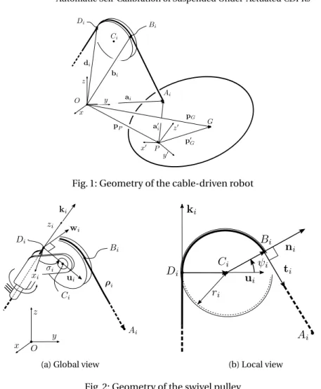
A generic 6-DoF under-actuated CDPR consists in a mobile platform connected to the base by n < 6 cables, which are actuated by motorized winches (Fig. 1). Ox y z is an inertial frame, whereas P x0y0z0is a mobile frame attached to the e-e. The platform pose is described by the position vector p_Pof P , and the rotation matrix R(φ,θ,χ) is parametrized by Tait-Bryant angles² = [φ,θ,χ]T according to the x y z convention. The platform generalized coordinates are thus p = [pP,²]T∈ R6.

Cables are modelled as massless and inextensible, and are guided by swivel pul-leys [15] to their attachment points Ai, i = 1,...,n on the platform (Fig. 2a). G is the

Fig. 1: Geometry of the cable-driven robot

(a) Global view (b) Local view

Fig. 2: Geometry of the swivel pulley

platform center of mass. If the coordinates of G and Ai in the mobile frame are de-scribed by vectorsPp_G0 andPa0_i, their coordinates in the inertial frame are:

p_G= pP+ p0G= pP+ RPpG0, ai= pP+ a0_i= pP+ RPa0_i (1) The i -th swivel pulley has center Ci, radius ri, and is mounted on a hinged sup-port, whose swivel axis ziis tangent to the pulley (Fig. 2a). Vector didefines the fixed position of point Di where the i -th cable enters the pulley’s groove and which is on the zi-axis. Unit vectors ii, ji, ki, associated with an additional fixed reference frame

Dixiyizi attached in Di, describe the orientation of each swivel pulley in Ox y z. The i -th cable exit point from the pulley groove is denoted by Bi and the vector ρi= Ai− Bi is tangent to the pulley.

In static conditions, if friction in the pulley hinges is negligible, vectors ziandρi define the pulley plane, forming the swivel angleσi with the coordinate plane xizi.

If uiand wiare unit vectors orthogonal to ki and to each other:

wi= −sin σiii+ cos σiji, ui= cos σiii+ sin σiji (2) the aforementioned static constraint can be analytically expressed as:

wi· (ai− di) = 0 (3)

which can be solved forσi(p), if the pose is assigned.

We defineψi∈ (−π, π) as the angle between ui and Bi− Ci (Fig. 2b). It is conve-nient to define two more unit vectors, orthogonal to wiand to each other:

ni= cos ψiui+ sin ψiki, ti= sin ψiui− cos ψiki (4) so that the i -th cable vector can be expressed as:

ρi= ai− di− ri(ui+ ni) = kρikti (5) where

kρik = li− ri(π − ψi) (6) is the rectilinear cable length, and li is the i -th total cable length, comprising the rectilinear part and the wrapped partBÚiDi. The tangency constraint betweenρiand the pulley can be expressed as:

ni· ρi= 0 (7)

which can be solved forψi(p), if the pose (and thus the swivel angle) are known. Onceψi(p) andσi(p) are determined, li(p) can be found from the geometrical constraint that the i -th cable imposes on the platform:

ρT

i ρi− kρik2= 0 (8)

whereρ_iis evaluated as in Eq. (5) and kρik as in Eq. (6).

2.2 Statics

For the purpose of this work, we will consider that the e-e is acted upon by a constant force only, e.g. gravity, which is parallel to the z axis and applied at point G. Thus, if the e-e mass is m, the gravitational acceleration is g , and ˜p_G0 is the skew-symmetric representation of the vector product, namely p0

G× = ˜pG0, the external wrench applied to the reference point P is W = −mg [k; ˜p0

Gk].

If all cables are taut, the static equilibrium equations of the e-e is:

JTT − W = 0 (9)

where T = [T1, ··· ,Tn]T, Ti is the cable tension, and J ∈ Rn×6is the Jacobian matrix of the constraints in Eq. (8), whose i -th row is Ji = [tT_i − tT_i ˜a0_i]. It is convenient to

partition J in a n × n matrix Ja and a n × (6 − n) matrix Ju, namely J = [JaJu], and vector W as W = [Wa; Wu], so that Eq. (9) can be rewritten as:

JT_aT − Wa=0 (10)

JT_uT − Wu=0 (11) The first part can be solved for T, thus yielding:

T = J−Ta Wa (12)

and the result can be substituted in the second part, thus obtaining the static equi-librium constraint of the platform:

JT_uJ−T_a Wa− Wu= 0 (13)

2.3 Forward Geometrico-Static Problem

The aim of the forward geometrico-static problem is to find the e-e pose, once the value of a suitable set of the robot’s internal joint variables is known. In the case that only cable length measurements are available, it is possible to formulate such a prob-lem by considering the n constraints in Eq. (8) and the 6 −n equations in Eq. (13) [1]. The resulting system of nonlinear equations is completely determined and, thus, can be numerically solved by using nonlinear solvers. Alternatively, if redundant mea-surements are available, one can (possibly) neglect the static constraint equations and replace them with additional kinematic constraint equations that are explicitly dependent on the measured variables [10]. This approach leads to a system of equa-tions that, depending on the number and the type of redundant measurements, can be completely determined or overdetermined (the system is never underdetermined, because static equilibrium constraints can always be accounted for).

In this paper, we assume that both cable lengths and swivel pulley angles can be measured. For the sake of generality, we formulate the forward geometrico-static problem by considering both 2n kinematic constraints, derived from Eqs. (3) and (8), and the 6−n static equilibrium constraints of Eq. (13), thus leading to an overde-termined system of 6 + n equations in 6 unknowns (namely, the generalized pose coordinates in p). By letting: F1(p) =    σ1(p) − σ∗1 .. . σn(p) − σ∗n   , F2(p) =    l1(p) − l1∗ .. . ln(p) − ln∗   , F3(p) = J T uJ−Ta Wa− Wu (14) whereσi(p) and li(p) can be easily calculated from Eqs. (3) and (8), andσ∗_i and l_i∗ are the corresponding measured values, the forward geometrico-static problem can be formulated as: F(p) =   F1(p) F2(p) F3(p)  = 0 (15)

This formulation leads to a fairly simple analytical formulation of the first-order dif-ferentiation of Eq. (15), as described in Section 3.

3 Initial-Pose Estimation Problem

In this section, the initial-pose estimation problem will be formulated by extending the work presented in [8]. If the under-actuated CDPR is equipped with incremental measurement devices on motors and swivel axes, i.e. incremental encoders, cable lengths and swivel angles at a generic pose pican be measured relatively to the initial valuesσ0_i and l_i0at pose p0, namely:

σ∗

i = σ

0

i+ ∆σ∗i (16)

l_i∗_{= li}0_{+ ∆li}∗ (17)

While∆σ∗_i and∆l_i∗are measures provided by the encoders,σ0_i and l_i0are generally unknown and are the objective of the self-calibration procedure. The direct geometrico-static problem in Eq. (15) can thus be expressed as:

F(σ0, l0, p) = 0 (18)

whereσ0= [σ01, ··· ,σ0n]T and l0= [l10, ··· ,ln0]T. This problem has 6 + n equations and 6 + 2n unknowns (σ0, l0, p), and it has generally an infinite number of solutions.

However, by assuming thatλ different measurement sets are available, that is:

σ∗

i ,k= σ

0

i+ ∆σ∗i ,k

l_{i ,k}∗ _{= li}0_{+ ∆li ,k}∗ k = 1,··· ,λ (19)

the following system of equations is obtained:

G(X) = G(σ0, l0, p1, ··· ,pλ) = [F(σ0, l0, p1); ··· ;F(σ0, l0, pλ)] = 0 (20) where X = [σ0; l0; p1; ··· ;pλ] ∈ R6λ+2n.

The system (20) has a total ofλ(6 + n) equations and 6λ + 2n unknowns. Thus, if

λ > 2, the initial-pose estimation problem is overdetermined and can be formulated

as a non-linear least-square optimization:

Xopt= arg min

X kG(X)k

2 ₍₂₁₎

This problem can be solved by employing numerical techniques, such as the Levenberg-Marquardt algorithm. The efficient solution of Eq. (21) relies on a reasonable initial solution guess Xg uess(see Section 4), and an analytical formulation of the Jacobian matrix in Eq.(20). While the former is fundamental for both the solution accuracy and the algorithm rapidity, the latter is critical only in terms of computational time.

∂G ∂X =                    −In×n 0n×n ∂σ(p1)/∂p 0n×6 · · · 0n×6 0n×n −In×n ∂l(p1)/∂p 0n×6 · · · 0n×6 0(6−n)×n 0(6−n)×n ∂F3(p1)/∂p 0(6−n)×6 · · · 0(6−n)×6 −In×n 0n×n 0n×6 ∂σ(p2)/∂p ··· 0n×6 0_{n×n −In×n} 0_{n×6 ∂l(p}2)/∂p ··· 0n×6 0_(6−n)×n 0_(6−n)×n 0_(6−n)×6 ∂F3(p2)/∂p ··· 0(6−n)×6 .. . ... ... ... . .. ... −In×n 0_n×n 0_n×6 0_{n×6 · · · ∂σ(pλ})/∂p 0_{n×n −In×n} 0_n×6 0_{n×6 · · · ∂l(pλ})/∂p 0_(6−n)×n 0_(6−n)×n 0_(6−n)×6 0_{(6−n)×6 · · · ∂F}3(pλ)/∂p                    (22)

where I_n×nand 0_n×nare the n×n identity and zero matrices, σ(pk) = [σ1(pk); ··· ;σn(pk)] and l(pk) = [l1(pk); ··· ;ln(pk)]. Manipulating Eqs. (3),(7) and (8) yields:

∂σi ∂p = · _wT i uT_i (ai− di) − wT_i ˜a0_iH uT_i (ai− di) ¸ , ∂li ∂p =£tTi −tTi ˜a0iH ¤ (23) where, respectively denoting cos x and sin x by cxand sx:

H =   1 0 s_θ 0 c_φ−sφc_θ 0 s_φ c_φc_θ   (24)

Finally, by considering that:

∂JT i ∂p = · ∂ti/∂p ˜a0 i(∂ti/∂p) −˜ti(∂a0i/∂p) ¸ , ∂W ∂p = −mg · 0_3×1 ˜ k˜r0_H ¸ (25) and: ∂ti ∂p= wisinψi∂σi ∂p + ni ∂ψi ∂p, ∂a0 i ∂p =£03×3 −˜a0iH ¤ (26) ∂ψi ∂p = · nT_i kρik − nT_i ˜a0_iH kρik ¸ (27)

∂F3/∂p can be evaluated according to the partition defined in Section 2.2 as:

∂F3 ∂p = ³∂JT u ∂p − J T uJ−Ta ∂JT a ∂p ´ J−T_a Wa+ JTuJ−Ta ∂Wa ∂p − ∂Wu ∂p (28)

4 Data Acquisition Algorithm

It is beyond the scope of this work to determine an optimal data acquisition algo-rithm. However, a practical one, which enables autonomous and safe operation of the CDPR during calibration, is provided hereafter. For this aim, cable tensions or alternatively motor torques are assumed to be measurable or at least estimated, and actively controlled by a suitable feedback system.

In the instant the robot is switched on, its pose is generally unknown. It is possibly unsafe to start the self-calibration process in this configuration. Then, it is useful to pre-determine a safe start configuration, in which every cable is taut and sufficiently long, so that it can be coiled and uncoiled, and the e-e may attain different poses. By assigning a start cable tension vector T0, the static problem (9) can be solved for p as

a non-linear system of six equations in six unknowns. Because of the non-linearity of the problem, a finite set of real solutions can be determined: this calculation may be done off-line and just once, i.e. during robot parameter calibration. Only stable solutions [4] among the possibly many available should be considered. Additionally,

T0may be selected so that only one stable solution exist.

In the following, we will consider a start cable tension vector leading to a unique stable solution of problem (9). Accordingly, a (computed) start pose p0,compis

unam-biguously determined, as well as start cable lengths l0_comp and swivel anglesσ0_comp. The real start pose p0attained by the CDPR can be fairly different from the ideal one

p0,comp, and its determination is the aim of the self-calibration procedure. A

maxi-mum cable tension vector Tmshould be set as well. The data acquisition algorithm objective is to ensure that every DoF of the e-e is varied during measurements, so that problem (21) is always well conditioned. The procedure workflow can be sum-marized as follows.

1. Start phase: command the CDPR so that cable tensions (or motor torques) quasi-statically reach the assigned value T0. When T0is reached and static conditions

are attained3, the j -th actuator is assigned an incremental cable tension (or mo-tor mo-torque) point, starting from j = 1. The change in a single actuamo-tor set-point ensures that the pose of the end-effector is different at any iteration, thus being effective, as well as practical and easy to implement;

2. Tensioning phase: quasi-statically move the CDPR by assigningλ/(2n) positive increments of magnitude∆T = 2n(Tj ,m− Tj ,0)/λ to the tension set-point of the

j -th actuator, namely T_{j ,k = Tj ,k−1+ ∆T , where T}j ,0is the j -th component of

T0. After each assignment k, the CDPR e-e could possibly oscillate during the

transition. When static conditions are attained, record measurements_∆σ∗

i ,kand ∆l∗

i ,k, for i = 1,··· ,n;

3. Detensioning phase: assignλ/(2n) negative increments of magnitude ∆T to the tension set-point of the j -th actuator, namely Tj ,k= Tj ,k−1− ∆T . When static conditions are attained, record measurements∆σ∗

i ,k and∆li ,k∗ , for i = 1,··· ,n. During the detensioning phase, the robot follows exactly the same cable tension (motor torques) set-points as in the tensioning phase: on a real machine, due to repeatability errors, this could lead to different cable lengths and swivel an-gles, which are possibly useful in the calibration procedure in order to minimize the repeatability error of the robot.λ/n measurement sets are thus obtained by varying a single actuator set-point;

3_{Notice that cable tensions are only used to lead the platform to poses where the robot is}

stable and kinematic measures can be accurately performed. They have no role in the op-timization problem solution, since they do not appear as variables in Eq. (21). They may be affected by appreciable errors without compromising the procedure, whereas platform stability plays a key role in the data acquisition process.

Table 1: Actuation unit properties i di[m] ri[m] Pa0_i[m] xi yi zi 1 h −2.030 −0.170 0.806 iT 0.025 h 0.020 −0.287 0.250 iT ey −ez −ex 2 h0.066 0.920 0.757 iT 0.025 h0.251 0.153 0.250 iT

−ex −ez −ey 3 h−2.043 2.241 0.738]

iT

0.025 h0.211 0.153 0.250 iT

−ey ez −ex

4. Increment phase: j = j + 1; if j ≤ n then go to point 2, otherwise the algorithm is finished becauseλ measurement sets have been recorded.

The initial guess for the solution of problem (21) is computed as:

Xg uess= £

σ0

comp; l0comp; p1,comp; ··· ; pλ,comp¤ (29) where pk,comp, k = 1,...,λ, can be evaluated by solving the static problem (9) with assigned tension Tk. Finally, by employing Xg uess,∆σ∗_k= [∆σ∗_1,k· · · ∆σ∗_n,k]T and ∆l∗

k= [∆l1,k∗ · · · ∆l∗n,k]

T _{for k = 1,··· ,λ, it is possible to determine Xoptas a solution of} (21). Ideally,_σ0_opt and l0_optshould converge to_σ0and l0, respectively.

5 Simulations and Experimental Results

A simulation example, developed in MATLAB®, aims at testing the efficiency of the optimization routine as a function ofλ and the different formulations of the Jaco-bian. Experimentation on a prototype shows the application of the method in a real-word scenario. The geometrical properties of a 3-cable 6-DoF under-actuated CDPR used for both simulation and experimentation are summarized in Table 1, where

ex= [1 0 0]]T, ey = [0 1 0]T and ez= [0 0 1]T are elements of the canonical basis of

SO(3). The platform mass is m = 8Kg, andPp0_G=£0 0 0.182¤Tm.

5.1 Simulation results

If the start tension vector T0=£40 40 40¤

T

N is assigned, the only stable solution of the static problem (9) is p0=£−1.363 0.963 −0.460 −0.056 −0.069 −0.557¤Tm, l0=

£1.470 1.509 1.543¤Tm, andσ0=£0.738 0.607 −0.799¤Trad. Since the simulation is based on a perfect data acquisition process, the above (theoretical) values of p0, l0

andσ0are the expected output of the optimization algorithm.

According to the procedure proposed in Section 4, several simulations were performed with different values of λ, i.e. λ = 12 ÷ 372. The initial guess Xg uess for the optimization solver was generated by considering a perturbed start ten-sion T0,per t = £46.9 23.9 32.6¤

T

N. In this case, the only stable solution of the static problem (9) yields p0,comp =£−1.648 0.740 −0.732 −0.246 0.179 −0.523¤

T m,

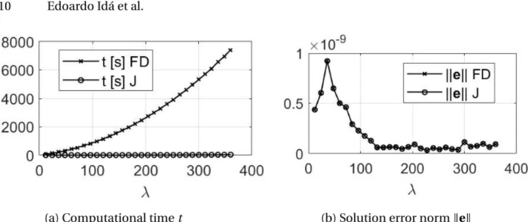
(a) Computational time t (b) Solution error norm kek Fig. 3: Simulation results comparing FD and J formulations

l0_comp =£1.468 1.914 1.802¤Tm, and σ0_comp = £0.926 0.684 −0.849¤Trad. Further-more, Tm=£80.0 80.0 80.0¤

T

N was set. Complete numerical data regarding Xg uess, for k = 1,··· ,λ, are omitted due to space limitations.

In the case of ideal measurements, a solution Xop tto the problem (21) is always found that is not only a minimum, but a real numerical zero. Solutions were com-puted in Matlab by using the lsqnonlin solver. Figure 3 shows the computational time and the norm of the error e = p0−p0,op tfor a variable numberλ of measurement sets,

in the case a finite-difference estimation (FD) or an analytical formulation (J) of the Jacobian. It is clear that the analytical formulation is crucial for the algorithm time-performance, whereas there is no noticeable difference in the numerical precision achieved by the two numerical formulations. Simulations also show that there are no advantages in acquiring an increasing number of data points for the initial-pose estimation. The norm of error e is consistent with the numerical tolerance.

5.2 Experimental results

The proposed data acquisition strategy and calibration method was tested on a pro-totype. Swivel angles were measured by 16-bit incremental encoders, mounted di-rectly on the swivel axes of pulleys, whereas cable lengths were estimated by using 20-bit incremental encoders on each motor axis and a kinematic model of the winch. Swivel pulleys were manufactured by FDM technology, thus limited, but not negli-gible, errors in their geometry and elasticity exist. Cables were coiled on IPAnema winches [16]. Clearance and elasticity in the winch components, as well as cable elas-ticity itself, are possible sources of error in the estimation of cable lengths.

In order to measure the real pose of the platform during experiments, 8 VICON Motion Capture Systems cameras were employed to track the position of 4 markers mounted on the robot platform.The accuracy of the measure is ±0.2mm for each di-mension of the marker (x, y, z), according to manufacturer specifications. In the end, the position of the reference point and the platform orientation were reconstructed from the recorded position of each marker.

Table 2: Experiments results i p0[mm,◦] p0,op t[mm,◦] kepk [mm] ke²k [◦] 1 h −1314 900 −355 −5.0 −4.8 −32.0 iT h −1324 906 −361 −4.5 −4.9 − 32.1 iT 13.4 0.5 2 h −1345 922 −322 −4.0 −3.6 −31.9 iT h −1347 913 −325 −4.2 −4.0 − 32.0 iT 9.9 0.4 3 h−1348 917 310 −4.1 −3.4 −32.1 iT h −1357 895 −310 −5.0 −3.6 −32.0 iT 23.4 0.9 4h−1349 917 −310 −4.1 −3.4 −32.0 iT h −1359 914 −307 −4.2 −3.5 −31.9 iT 11.5 0.2 5h_{−1344 913 −314 −4.2 −3.6 −32.0}iT h_{−1348 918 −315 −4.0 −3.9 −31.9}iT 5.7 0.4

Because of the lack of force sensors in the robot set-up, motor torques were em-ployed instead of cable tensions for the implementation of the algorithm presented in Section 4. The start tension vector and maximum cable tensions were set to T0=

£40.0 40.0 40.0¤TN and Tm=£80.0 80.0 80.0¤ T

N, respectively, and converted in mo-tor mo-torques according to static equilibrium of the cable transmissions. In the end,

λ = 60 was chosen as a trade-off between accuracy of the initial-pose estimation and

data-acquisition speed.

The results of five experiments are reported in Table 2, where p0is the real

start-ing pose, as measured by the motion trackstart-ing system, p0,op t is the estimated

start-ing pose resultstart-ing from the solution of the problem (21), kepk = kp0− p0,op tk is the

reference position error norm and ke²k = k²0− ²0,op tk is the norm of the error of the

orientation parameters. Positions are expressed in millimeters and angles in degrees. The execution of the calibration procedure required, on average, 4 min for the data acquisition procedure, and 2.5 s for the initial-pose estimation by using the analytical formulation of the Jacobian (16 min by using a finite-difference estimation).

During experiments, it was observed that the orientation of the swivel pulley axes plays a crucial role for the conditioning of problem (21). Pulley orientations were set in order to achieve the best possible results with the robot architecture at hand, but are not optimal. Nonetheless, the results are satisfactory by considering the mod-elling simplification and the hardware at hand.

6 Conclusions

This paper presented an automatic self-calibration method for suspended under-actuated CDPRs, extending the method proposed in [8]. An analytical formulation of the problem was developed and an autonomous procedure to calibrate the initial-pose of the CDPR by means of incremental measurements of cable lengths and swivel angles was shown. Experimental results on a prototype show that the applica-tion of the proposed method is promising, but it needs refining in order to achieve a higher accuracy. In particular, the optimal orientation of the swivel pulleys and the effect of uncertainties in the measurements will be investigated in the future.

References

1. Abbasnejad, G., Carricato, M.: Direct geometrico-static problem of underconstrained cable-driven parallel robots with n cables, IEEE Transactions on Robotics, vol. 31, no. 2, pp. 468-478 (2015).

2. Berti, A., Merlet, J.P., Carricato, M.: Solving the direct geometrico-static problem of under-constrained cable-driven parallel robots by interval analysis, The International Journal of Robotics Research, vol. 35, no. 6, pp. 723-739 (2016).

3. Borgstrom, P.H., Jordan, B.L., Borgstrom, B.J., Stealey, M.J., Sukhatme, G.S., Batalin, M.A., Kaiser, W.J.: Nims-pl: A cable-driven robot with self-calibration capabilities, IEEE Trans-actions on Robotics, vol. 25, no. 5, pp. 1005-1015 (2009).

4. Carricato, M., Merlet, J.P.: Stability Analysis of Underconstrained Cable-Driven Parallel Robots, IEEE Transactions on Robotics, vol. 29, no. 1, pp. 288-296 (2013).

5. Daney, D., Andreff, N., Chabert, G., Papegay, Y.: Interval method for calibration of parallel robots: Vision-based experiments, Mechanism and Machine Theory, vol. 41, no. 8, pp. 929-944, (2006).

6. Hwang, S.W., Bak, J.H., Yoon, J., Park, J.H., Park, J.O.: Trajectory generation to suppress oscillations in under-constrained cable-driven parallel robots, Journal of Mechanical Sci-ence and Technology, vol. 30, no. 12, pp. 5689-5697 (2016).

7. Idá, E., Berti, A., Bruckmann, T., Carricato, M.: Rest-to-rest trajectory planning for planar underactuated cable-driven parallel robots, in Cable-Driven Parallel Robots, C. Gosselin, P. Cardou, T. Bruckmann, and A. Pott, Springer, pp. 207-218 (2018).

8. Lau, D.: Initial length and pose calibration for cable-driven parallel robots with relative length feedback, in Cable-Driven Parallel Robots, C. Gosselin, P. Cardou, T. Bruckmann, and A. Pott, Springer, pp. 140-151 (2018).

9. Lin, J., Liao, G.: Design and oscillation suppression control for cable-suspended robot, in 2016 American Control Conference, pp. 3014-3019 (2016).

10. Merlet, J.P.: Direct kinematics of cdpr with extra cable orientation sensors: The 2 and 3 cables case with perfect measurement and ideal or elastic cables, in Cable-Driven Parallel Robots, C. Gosselin, P. Cardou, T. Bruckmann, and A. Pott, Springer , pp. 180-191 (2018). 11. Miermeister, P., Pott, A.: Auto calibration method for cable-driven parallel robots using

force sensors, in Latest Advances in Robot Kinematics, J. Lenarcic and M. Husty, Springer, pp. 269-276 (2012).

12. Miermeister, P., Pott, A., Verl, A.: Auto-calibration method for overconstrained cable-driven parallel robots, in ROBOTIK 2012; 7th German Conference on Robotics, pp. 1-6 (2012).

13. Nubiola, A., Slamani, M., Joubair, A., Bonev, I.A.: Comparison of two calibration methods for a small industrial robot based on an optical CMM and a laser tracker, Robotica, vol. 32, no. 3, pp. 447-466 (2014).

14. Pott, A.: An algorithm for real-time forward kinematics of cable-driven parallel robots, in Advances in Robot Kinematics: Motion in Man and Machine, J. Lenarcic and M. M. Stanisic, Springer, pp. 529-538 (2010).

15. Pott, A.: Influence of pulley kinematics on cable-driven parallel robots, in Latest Advances in Robot Kinematics, J. Lenarcic and M. Husty, Springer, pp. 197-204 (2012).

16. Pott, A., Mütherich, H., Kraus, W., Schmidt, V., Miermeister, P., Verl, A.: IPAnema: A fam-ily of Cable-Driven Parallel Robots for Industrial Applications,in Cable-Driven Parallel Robots, T. Bruckmann and A. Pott, Springer, pp. 119-134 (2013).

17. Zarei, M., Aflakian, A., Kalhor, A., Masouleh, M.T.: Oscillation damping of nonlinear con-trol systems based on the phase trajectory length concept: An experimental case study on a cable-driven parallel robot, Mechanism and Machine Theory, vol. 126, pp. 377-396, (2018).