Comparisons of an aerosol transport model with a 4-year analysis of summer aerosol optical depth retrievals over the Canadian Arctic

(1)

Faculté des lettres et sciences humaines Département de géomatique appliquée

Université de Sherbrooke

Comparisons of an aerosol transport model with a 4-year

analysis of summer aerosol optical depth retrievals over the

Canadian Arctic

« Comparaisons d'un modèle de transport d'aérosols avec une

analyse de 4 ans de mesures estivales d’épaisseur optique

d'aérosols dans l'Arctique canadien »

Sareh Hesaraki

Mémoire présenté pour l’obtention du grade de Maître en sciences géographiques (M. Sc.), cheminement télédétection

(2)

Composition du jury

Ce mémoire a été évalué par un jury composé des personnes suivantes :

Prof. Norman T. O’Neill

Dép.de géomatique appliquée, Université de Sherbrooke Directeur de recherche

Prof. Alain Royer

Dép.de géomatique appliquée, Université de Sherbrooke Examinateur

Prof. Martin Aubé

Dép. de physique, Cegep de Sherbrooke Physics department of Bishop's University Dép.de géomatique appliquée, Université de Sherbrooke

(3)

i

Abstract

This is a study concerning comparisons between the Dubovik Aerosol optical depth (AOD) retrievals from AEROCAN (ARONET) stations and AOD estimates from simulations provided by a chemical transport model (GEOS-Chem : Goddard Earth Observing System Chemistry). The AOD products associated with the Dubovik product are divided into total, fine and coarse mode components. The retrieval period is from January 2009 to January 2013 for 5 Arctic stations (Barrow, Alaska; Resolute Bay, Nunavut; 0PAL and PEARL (Eureka), Nunavut; and Thule, Greenland). We also employed AOD retrievals from 10 other mid-latitude Canadian stations for comparisons with the Arctic stations.

The results of our investigation were submitted to Atmosphere-Ocean. To briefly summarize those results, the model generally but not always tended to underestimate the (monthly) averaged AOD and its components. We found that the subdivision into fine and coarse mode components could provide unique signatures of particular events (Asian dust) and that the means of characterizing the statistics (log-normal frequency distributions versus normal distributions) was an attribute that was common to both the retrievals and the model.

Keywords : Aerosol, Aerosol Optical Depth (AOD), GEOS-Chem, AEROCAN, Dubovik inversion

(4)

ii

Résumé

Cette étude compare des épaisseurs optiques d’aérosols (AOD) à 5 stations arctiques d’AEROCAN (AERONET), obtenues d’une part à l’aide de l’algorithme d'inversion de Dubovik appliqué à des mesures in situ, et d’autre part du modèle de transport chimique (GEOS-Chem : Goddard Earth Observing Système Chemistry). Les produits d’AOD associés à l’algorithme d’inversion sont divisés en composantes totales, fines et grossières. Pour chacune des 5 stations (Barrow, Alaska, Resolute Bay, au Nunavut, 0PAL et PEARL (Eureka), Nunavut, et Thulé, au Groenland), la période de récupération est de janvier 2009 à janvier 2013. Nous avons également utilisé les mesureurs d’AOD de dix autres stations canadiennes de latitudes moyennes, à des fins de comparaison.

Les résultats de l’étude ont été soumis à la revue Atmosphere-Ocean. Pour résumer brièvement ces résultats, le modèle a généralement, mais pas toujours, eu tendance à sous-estimer l'AOD moyenne et de ses composantes. Nous avons constaté que la subdivision en composantes fine et grossière pourrait fournir des signatures uniques d'événements particuliers (poussière asiatique) et que les moyens de caractériser des statistiques (les distributions de fréquence log-normale versus les distributions normales) était un attribut qui était commun aux deux les mesureurs et le modèle.

(5)

iii

List of Figures

Figure 1. Map showing the five Arctic stations whose data was used in this study as well as the 10 southern stations whose data was employed for purposes of comparison with the Arctic data. ... 13 Figure 2. Normal and log-normal fit comparisons for AERONET and GC AOD histograms (a) Linear and lognormal histograms (left and right-hand graphs, respectively) for AERONET at λ = 500 nm and GC at λ = 550 nm (top and bottom rows respectively), (b) An example of how to employ the traditional means of reporting sun photometry AOD statistics (linear mean and standard deviation) to extract parameters that are representative of the lognormal distribution. In this illustration the linear mean and standard deviation are used to estimate the geometric mean of the histogram by calculating the latter from the lognormal parameterization (equations (2) and (3))... 20 Figure 3. Comparison between various types of monthly averages (black and purple) and the monthly averages (green) of Tomasi et al. (2015). The Tomasi AOD averages represent Level 2.0 extinction data. The purple curve shows the averages for the MYSP. The error bars are standard deviations. ... 23 Figure 4. 〈 τa 〉 (averaged over the 2009 to 2112 MYSP) as a function of month for the Arctic stations compared with the analogous averages for the 10 southern stations. The error bars are standard deviations ... 25 Figure 5. 〈τf 〉, 〈τc 〉 and 〈τa 〉 (monthly averages over the 2009 to 2112 MYSP) and modelled values (〈τf,GC〉,〈τc,GC〉 and 〈τa,GC 〉) as a function of month. The error bars are standard deviations. ... 26 Figure 6. Coefficient of determination between modelled and retrieved daily AOD means for the ensemble of all sites ("all") and for individual sites. The error bars are the standard deviations corresponding to one standard deviation of Fisher's z transformation distribution (see Siegel, 1961, for example). ... 28 Figure 7. 〈τf 〉 Fine mode monthly averages over the MYSP for all 5 Arctic sites. The error bars are the standard deviations. ... 30 Figure 8. 〈τc〉 Coarse mode monthly averages over the MYSP for all 5 Arctic sites. The error bars are the standard deviations. ... 32 Figure 9. Scattergrams in log-log space of the model versus AERONET retrievals (a for file mode, b for coarse mode and c for total AOD) based on a linear regression (bold line) and logarithmic regression (thicker dashed line) for the ensemble of all sites. The very short dashed line is the y=x line. ... 45 Figure 10. Intra-annual variation of fine AODs over the MYSP ... 46 Figure 11. Intra-annual variation of coarse AODs over the MYSP ... 47

(8)

vi

List of Tables

Table 1. AEROCAN/AERONET sites employed in this study. ... 14 Table 2. Ensemble monthly means of Level 1.5 and Level 2.0 AOD components and the

(9)

vii

Preface

This document presents the results of a Master's thesis carried out at l’Université de Sherbrooke at the Department of Applied Geomatics under the supervision of Professor Norm O’Neill. This thesis is based on an article entitled ‘Polar summer comparisons of a chemical transport model with a 4-year analysis of fine and coarse mode aerosol optical depth retrievals over the Canadian Arctic’ that was submitted to a peer reviewed journal, Atmosphere-Ocean on August.29, 2016. Sareh Hesaraki is the first author with Norman T. O'Neill, Glen Lesins, Auromeet Saha, Randall V. Martin, Vitali E. Fioletov, Konstantin Baibakov, and Ihab Abboud being the co-authors.

(10)

viii

Acknowledgements

My deepest gratitude is to my director, Professor Norm O’Neill. I have been amazingly fortunate to have an advisor who gave me the freedom to explore on my own and at the same time the guidance to recover when my steps faltered.

I am also indebted to Professor Glen Lesins as well as Professor Randall Martin and his research group at Dalhousie University : this work would not have been possible without their help. I would like to acknowledge the principal investigators of the AERONET sites whose data I used in my Master's project.

The results of this study are part of a larger NSERC – CCAR (National Sciences and Engineering Research Council - Climate Change and Atmospheric Research) funded project called NETCARE (NETwork on Climate and Aerosols : addressing key uncertainties in Remote Canadian Environments).

(11)

CHAPTER 1. General introduction

1.1 Atmospheric aerosols

Atmospheric aerosols are small particles whose size (radius) varies from ~ 0.001 μm to 100 μm and which are in solid, liquid or mixed phase (see Hinds, 1998 for fundamental text on the nature of aerosols and their measurement). These particles have impacts on human health inasmuch as they are commonly associated with pollution as well as important impacts on climate change. According to the authors of the IPCC, working group I report, aerosols represent the largest uncertainty in radiative forcing calculations (IPCC, 2013). This uncertainty manifests itself as the uncertainty in describing the direct and indirect effect of aerosols. The former effect, which is largely a cooling phenomenon, results from aerosol backscattering of solar radiation into space. The latter effect is the consequence of aerosols acting as condensation or ice forming nuclei for cloud particles and the fact that the properties of those cloud particles are dependent on the properties of the aerosol nuclei.

The aerosol parameters considered in this study, are of two different types (see the introduction section of the submitted paper in the next chapter for more details). These parameters can be extensive in nature inasmuch as they vary with the number (amount) of aerosols : typically such properties are rather localized in space and time and are subject to high frequency variations in both those dimensions. Alternatively, they can be intensive in nature (per particle properties) : intensive properties tend to be more regional in space inasmuch as they are associated with the type (source) of the aerosol or hence with the type of air mass. The most important extensive parameter in our research is AOD (Aerosol Optical Depth) while the important intensive aerosol parameters are particle size and particle nature (nature being represented by refractive index in an optical sense and composition in a microphysical sense).

The research carried out for this thesis was associated with a sub-project of NETCARE (Abbatt, 2012). NETCARE is a collaborative project involving academic participants from a number of Canadian universities as well as government participants from Environment Canada (EC) and The Department of Fisheries and Oceans Canada (DFO).

(12)

2

1.2 Different types of aerosols and their sources

According to Hinds (1998), aerosols can be divided into different size categories: nucleation mode (0.001 μm – 0.01μm radius), Aitken mode (0.01μm – 0.1μm), accumulation mode (0.1μm - 1μm) and coarse mode (>1μm). Aerosols come from natural and anthropogenic sources. In terms of significant optical effects in the visible and near infra-red region these four modes essentially reduce to the accumulation (fine) mode and the coarse mode (O'Neill et al., 2001). Natural aerosols have diverse origins, including, for example volcanic eruptions, wild fires, wind impacted mineral dust over deserts, and sea salt from sea spray. Anthropogenic aerosols such as sulphates, nitrates and carbonaceous aerosols come mainly from combustion processes (Jacob, 1999).

Both natural and anthropogenic aerosols can be grouped into two categories : primary and secondary aerosols. Primary aerosols are mostly coarse mode particles emitted directly into the atmosphere by disintegration and / or dispersion of plant, and animal matter (or the microbes from different living or non-living surfaces). Fine mode secondary aerosols, however, begin as gases which subsequently form aerosols after gas to particle conversion processes (see Seinfeld & Pandis, 2006 for a general reference on aerosol types). In general, the subdivision into fine and coarse mode components is important for understanding the dynamics of aerosols since the separate modes generally represent independent types of aerosols

1.3 Aerosol spatio-temporal simulation using chemical transport models

Concentrations of aerosol (and other atmospheric constituents) can be estimated from models without, in the first instance, the direct use of observations. Chemical Transport Models (CTMs) simulate the temporal and spatial evolution of aerosol and gaseous compounds using meteorological data sets, emission inventories, as well as the physical and chemical laws that govern the behaviour of atmospheric constituents (Van Donkelaar et al., 2012). GEOS–Chem (the global CTM that we employed in our paper) has proven to be useful in analyzing atmospheric observations and to achieve a better understanding of aerosol dynamics on global and regional scales. The NETCARE strategy, with respect to the GEOS-Chem model, is to test various approaches and algorithms, and subsequently

(13)

3

recommend mature algorithms to be implemented in the models that simulate aerosol dynamics across the Canadian domain (Abbatt, 2012).

1.4 Objectives and hypothesis of the mémoire

Model simulations are widely used to achieve a more universal understanding of the dynamics of aerosols and their impact on climate change and air quality (Martin et al., 2010). These simulations involve complex inputs, processes, scaling considerations, etc. that, at one level or another must be compromised by the limitations of available computational resources as well as the limitations in our understanding of the basic mechanisms that influence the spatio-temporal evolution of aerosol properties. They therefore must be compared with aerosol measurements and adapted to the reality defined by those measurements. The information obtained from local, regional or global scale remote sensing of aerosols is arguably the most important model comparison source for measurements of aerosol models.

The present work falls within Activity 4 of the NETCARE program ("Implications of Measurements on Simulations of Atmospheric Processes and Climate.). Verifying the aerosol predictive capabilities of the GEOS-Chem model in comparisons with AERONET/AEROCAN retrievals of total, fine and coarse mode AODs was our objective within the larger context of Activity 4).

The GEOS-Chem capability of predicting the important (and robust) aerosol optical parameter of AOD, within the error uncertainty of the measurements, is the basis of the hypothesis that we sought to validate within the context of this study. Realistically we hoped to employ monthly means and the associated (natural) standard deviation of the measurements and the models as significance constraints on the intercomparability of total, fine and coarse mode AODs (where to total AOD is simply the sum of the fine and coarse mode AODs).

1.5 Overview of the article submitted as part of this mémoire

The climate behaviour of aerosols and their pollution effects in high latitude regions like the Arctic are not well known. Understanding the behaviour of aerosols in remote regions is important for modellers who wish to adequately characterize the meteorological scale

(14)

4

pollution impacts of aerosols as well as the longer term climate impacts in a region where such impacts are known to be magnified (IPCC technical summary of working group 2). The article that follows (Chapter 2) addresses certain elements of NETCARE Activity 4 ("Implications of measurements on simulations of atmospheric processes and climate" as defined in Abbatt, 2012). Future modifications of the paper during the revisions phase of the journal review will take into account some points to improve that were noted by the members of the mémoire jury.

The principal objective of the paper is to compare the polar summer simulations of a chemical transport model (GEOS-Chem) with a climatology of total, fine and coarse mode AOD retrievals over five Canadian Arctic stations. These retrievals depend on measurements of spectral AOD and sky radiance acquired by CIMEL instruments of the AEROCAN / AERONET network and the fundamental concept that much of aerosol optical behaviour can be understood in terms of fine / coarse bimodal size distributions (O’Neill et al., 2001). Comparisons with the model exploit its ability to subdivide aerosol types into fine and coarse mode components and, in turn, their fine and coarse mode AODs. The most important contribution of the paper relates to the fact that the coarse mode retrievals, even though their relative errors are very large, are a fairly unique indicator of what is likely Asian dust because (a) the timing is right (April), (b) GEOS-Chem says the same thing (and says that the coarse mode AODs are dominated by dust), (c) the separation into fine and coarse mode allows a very weak signal (c from the retrievals <~ 0.01) to be discriminated from the background in spite of the fact the expected errors of the retrieval method (something bigger than the typical CIMEL AOD errors of 0.01 to 0.02) are competitive if not larger than the nominal c values, (d) that GEOS-Chem coarse mode AODs are significantly correlated with coarse mode retrievals (the correlations were marginal for total AODs, so division into coarse and fine modes was a significant step), (e) that people generally don’t think of this nuanced means of verifying a model and that there is little in the literature related to an evaluation of that nature that we are aware of. It was also demonstrated that both the measurements and the model were characterized by frequency distributions that were lognormal and that this characteristic led to better model vs retrieval correlations in log-log space.

(15)

5

CHAPTER 2. Comparisons of an aerosol transport

model with the analysis of aerosol optical depth

retrievals over the Canadian Arctic

Paper title:

Polar summer comparisons of a chemical transport model with a 4-year

analysis of fine and coarse mode aerosol optical depth retrievals over the

Canadian Arctic

(Les comparaisons d'été polaires d'un modèle de transport chimique avec

une analyse de 4 ans des mesureurs d’épaisseur optique des aérosols en

composantes fines et grossières dans l'Arctique canadien)

Paper submitted to the journal of Atmosphere-Ocean on August 29, 2016

Sareh Hesaraki

1*

_{, Norman T. O'Neill}

1

_{, Glen Lesins}

2

_{, Auromeet Saha}

1

_,

Randall V. Martin

2,3

_{, Vitali E. Fioletov}

4

_{, Konstantin Baibakov}

5

_{, Ihab}

Abboud

4

1. Centre d’Applications et de Recherches en Télédétection, Université de Sherbrooke, Sherbrooke, QC, Canada.

2. Department of Physics and Atmospheric Science, Dalhousie University, Halifax, N.S. Canada.

3. Also at Harvard-Smithsonian Canter for Astrophysics, Cambridge, Massachusetts, United States.

4. Environment and Climate Change Canada (ECCC), Toronto, ON, Canada. 5. National Research Council Canada, Flight Research Laboratory, Ottawa, Canada.

(16)

6

Abstract

We compared AERONET retrievals of total, fine-mode (sub-micron), and coarse-mode (super-micron) aerosol optical depth (AOD) with simulations from a chemical transport model (GEOS-Chem) across five Arctic stations and a four year, Polar summer, sampling period. It was determined that the AOD histograms of both the retrievals and the simulations were better represented by a lognormal distribution and that the successful simulation of this empirical feature as well as its consequences (including a better model versus retrieval coefficient of determination in log-log AOD space) represented a general indicator of model evaluation success. Seasonal (monthly averaged) AOD retrievals were sensitive to how the averaging was performed: this was ascribed to the presence of highly variable fine mode smoke. The retrieved and modelled station-by-station fine mode AOD averages showed a peak in April / May which decreased across the summer period while the model underestimated the fine mode AOD by an average of about 0.01. Both the retrievals and simulations showed seasonal coarse mode AOD variations with a peak in April / May that was attributed to Asian dust. The success in capturing such weak seasonal events helps to confirm the relevance of the fine / coarse mode separation and the validity of model estimates in the Arctic.

Keywords: AERONET, Aerosol Optical Depth, Arctic, Chemical Transport Model, GEOS-Chem

(17)

7

2.1. Introduction

The IPCC (2013) affirmation concerning the importance of understanding aerosol contributions to the direct and indirect effect is of particular significance over the Arctic where climate change impacts are known to be magnified. In order to properly analyse aerosol processes and emission modelling in chemical transport models (CTMs) one needs to develop a reliable and varied measurement program to exercise as many of the aerosol functionalities as possible. Ground-based sun photometry measurements of aerosol optical depth (AOD) and sky radiance measurements represent key components of such a measuring program since they provide vertically averaged, robust parameters that define the macroscale, 1st order comparative constraints that models must satisfactorily simulate.

A climatological-scale analysis of AOD and its derivative products represents a basis of model comparison that gives perspective to more spatially and temporally demanding (event scale) comparisons. Such analyses can permit one to effectively filter out information about the most robust and fundamental mechanisms that control aerosol behaviour. Also, the AOD contamination impact of clouds and other sources of sun photometry error as well as the AOD computation impact of model limitations such as spatial resolution and time-step resolution are often dampened by carrying out comparisons at climatological scales.

The aerosol optical properties derived from sun photometry are predominantly constrained by a simple concept of bimodality : the detectable optical effects are largely driven by a bimodal (volume) particle size distribution (PSD) consisting of a fine mode or submicron component and a coarse mode or super micron component (see, for example, Whitby et al., 1972 for an earlier statement on the microphysical bimodality of the volume PSD and O'Neill et al., 2001 for a discussion of the optical bimodality). This concept represents a higher order but (still) robust approach relative to the classical Angstrom approximation for which the aerosol model is a simple, monotonically decreasing PSD (a Junge distribution for which the volume PSD, varying as 𝑟−å_{yields an}

AOD spectrum that varies as −å : å being the classical Angstrom exponent determined from a multi-band, log(AOD) versus log (λ regression)).

(18)

8

The bimodality concept means that one can divide aerosol optics into total, fine and coarse mode AODs, Angstrom exponents and their derivative (𝜏_𝑎, 𝛼, 𝛼′; 𝜏_𝑓, 𝛼_𝑓, 𝛼_𝑓′; 𝜏_𝑐, 𝛼𝑐, and 𝛼𝑐′ respectively, c.f. O'Neill et al., 2001). This presents an alternative, and

arguably more natural means, of evaluating columnar CTM outputs whose microphysics packages are (appropriately) based on fine and coarse mode aerosol species. Bi-modality represents a purer apportionment into extensive (quantity dependant) and intensive (per particle) optical properties (𝜏𝑎, 𝜏𝑓, 𝜏𝑐 and 𝛼, 𝛼𝑓, 𝛼𝑐, etc respectively).

Model evaluation and comparison in the literature is largely based on comparisons of AOD and å as well as speciated surface concentrations. In the Arctic, Hardenberg et al., (2012) compared AODs and regression Angstrom exponents simulated by two global models (ECHAM-HAM and TM5) with AODs extracted from the Polar AOD network & MODIS data over 6 Arctic stations for a sampling period extending from 2001 to 2006. They found that the models reproduced good estimates of Angstrom exponent but significantly underestimated the measured AODs. Breider et al. (2014) compared seasonal GEOS-Chem estimations of Arctic AOD with AODs measured at 8 Arctic stations for a sampling period of 1999 -2011. They observed that the model had succeeded in simulating AERONET AODs and provided model-based, speciation insight into how the constituent components would have contributed to the total AOD (including a general apportionment into natural and anthropenic aerosols). Shindell et al. (2008) and Eckhardt et al. (2015) carried out multi-model comparisons with surface aerosol concentrations measured in the Arctic. A notable feature of Shindell's comparisons was the large amount of variation in seasonal concentration between the estimates of different models (attributed to differences in aerosol and chemical physical processing, including removal). Eckhardt et al. (2015) noted large model variation (for sulfates) over the Arctic and observed that the models appeared to capture BC and sulfate concentrations while struggling to capture the extremes of the seasonal variation of the surface concentrations (notably the higher concentrations of the Arctic Haze in the springtime and the lower concentrations characteristic of the summertime).

In this paper we performed seasonal (monthly resolution) comparisons between the species dependent AODs simulated by a community CTM (GEOS-Chem) and AERONET sun photometry / radiometry retrievals of total, fine and coarse mode optical

(19)

9

depths over sites in or near the Canadian Arctic. The comparisons were carried out across a multi-year sampling period (MYSP) of 4 years (2009 – 2012). One of our major goals was to demonstrate the advantages of such an approach within a context of more traditional comparisons with generic AODs and Angstrom exponents. The investigation also includes an analysis of the most relevant means of presenting statistical results for both retrievals and simulations.

2.2. Background

2.2.1 Sun photometry and sky radiometry

The sun photometry / sky radiometry capabilities of the AERONET network provide classical measurements of spectral AOD in the solar extinction mode and angular measurements of sky radiance in the almucantar mode (Holben et al., 2001). The spectral AOD mode provides robust microphysical and / or optical retrievals with limited degrees of freedom while the combination of spectral AOD and sky radiance measurements provides microphysical and/or optical retrievals of multiple degrees of freedom (see Twomey & Howell, 1967 for a general discussion on, respectively, the number of degrees of freedom in "transmission" and "forward scattering" mode). In the extinction mode one can employ an algorithm such as the (Spectral Deconvolution Algorithm) SDA (O'Neill et al., 2003) to extract 𝜏𝑎, 𝜏𝑓, and 𝜏𝑐 at a reference wavelength of 500 nm (the

AERONET standard). In extinction / sky radiance mode one can extract particle size distribution and refractive index (Dubovik et al., 2000) and employ these results to compute 4-channel spectra of 𝜏𝑎, 𝜏𝑓, 𝜏𝑐which can be interpolated to a reference

wavelength such as 500 nm. The two sets of quantities are very similar but the SDA represents a spectral retrieval approach while the Dubovik retrieval literally divides the retrieved particle size distribution at a specific radius (c.f. O’Neill et al., 2003).

2.2.2 Averaging and standard deviation statistics

― Averaging nomenclature

In general, we will let < 𝜏_𝑥 > and 𝜎_𝑥 represent the arithmetic average and standard deviation across any averaging bin. These statistical parameters clearly depend on

(20)

10

conditions such as site, year, etc. Rather than overload the nomenclature with more subscripts, we will explain the context depending on the case being considered. Similarly, we will represent the geometric mean and standard deviation (that result from averages and standard deviations of log (𝜏_𝑥) by 𝜏_𝑔,𝑥 and 𝜇_𝑥. In the following section we discuss some implications of the averaging scheme (for this particular section only, we used a more elaborate subscripting scheme to help clarify the details of successive averaging).

― Averaging procedure and the interpretation of successive averaging

At any statistical level in this work we calculated an average or a standard deviation by employing all individual retrievals in any "averaging bin" (days, months, years, stations etc.). While one can debate the merits of any given averaging approach (see Levy et al., 2009, for example), the approach of employing individual measurements does have the distinct advantage of providing a clear point of reference for the averaging chain. Given this statistical protocol, it behoves one to be clear on how the relationship between successive averages across different averaging bins can be interpreted (simply because it is an inevitable question which arises as one statistically processes the data).

It is easy to demonstrate that requiring averages that employ all original measurements for a given averaging bin equates to a higher level average (monthly average, for example) being the weighted average of lower level averages (daily averages, for example) where the weights are the normalized number of measurements that contributed to the lower level averages (normalized number of measurements per day for our particular example). Thus the monthly AOD average of daily averages across month "k" would be: 𝜏_𝑥,𝑘 = ∑ 𝜔_𝑘,𝑗 𝜏_{𝑥,𝑘,𝑗} 𝐽𝑘 𝑗=1 where 𝜔_𝑘,𝑗 = 𝑁𝑘,𝑗 𝑁_𝑘 (1)

where 𝜏_{𝑥,𝑘,𝑗} and 𝑁_𝑘,𝑗 represent respectively the measurement and the number of measurements acquired on day "j" of month "k" and 𝑁_𝑘 is the total number of measurements during month "k" (we could have also proceeded by considering the means of 𝑙𝑜𝑔 (𝜏_𝑥,𝑘) as per the section below on lognormal distributions). An analogous relation

(21)

11

would be then employed to proceed up another level of successive averaging (which could be, for example, averaging across all stations for a given month "k"). It is also easy to show that the average obtained for a given set of averaging bins is independent of the order of the averaging (for example, monthly averages for a given year and station to yearly averages for a given station to station averages across the total ensemble (total MYSP data set) of retrievals can be performed as monthly averages to station averages to yearly averages and the result would be the same). This commutativity property applies only to the measurement-frequency weighting scheme as defined in equation (1) and not the general-purpose type of weighting schemes discussed in Levy et al. (2009).

― Lognormal versus normal representations

Various investigations in the literature have led to the observation that AOD histograms are better represented by a lognormal distribution as opposed to a normal distribution (which means that the AOD histogram is more realistically represented by a normal or Gaussian curve in logarithmic space and a long-tailed, positively skewed curve in linear space). These investigations include those of O’Neill et al. (2000), Knobelspiesse et al. (2004) and Perrone et al. (2005) for sun photometric data, Matthias et al. (2004) for lidar-retrieved AODs and Ignatov and Stowe (2002) for satellite-lidar-retrieved AODs. In terms of Arctic AOD multi-year analyses, the long-tailed, positively skewed asymmetry typical of a lognormal distribution appears in the histograms of Tomasi et al. (2015). In spite of this evidence for lognormality, the persistent if understandable inertia of historical reporting means that the AOD community, including some, if not all, of the co-authors of this paper, continue to report arithmetic statistics rather than geometric statistics. Basically this amounts, respectively, to reporting AOD statistics as the arithmetic mean and standard deviation1_{< 𝜏}

𝑥> ± 𝜎( 𝜏𝑥 ) rather than as the geometric mean and standard

deviation, 𝜏_𝑥,𝑔 × 𝜇_𝑥±1_{(or some related form depending on the desired probability}

metric). The latter expression is almost invariably a better representation of the AOD histogram (as well as derived parameters such as the median and peak values). This fact has non-trivial consequences: a climate modeller, for example, who wanted to report the

(22)

12

most probable AOD of a future AOD distribution would be distinctly incorrect in tying the objective analysis to an assumption that < 𝜏_𝑥 > was the most probable value.

The inertia of traditional reporting protocols aside, the geometric mean and standard deviation approach is rarely used because people are generally not as comfortable with logarithmic statistics as they are with linear statistics (and / or because they are not aware of the simple formulation above). In any event, the more relevant geometric statistics can be retrieved from the arithmetic statistics. It is easy to show (from Table 1 of O'Neill et al., 2000) that the former can be related to the latter:

𝜏_𝑔,𝑥 = < 𝜏_𝑥> exp (− ln2_(𝜇 𝑥⁄2)) where, (2) 𝜇𝑥 = exp [√ln (1 + ( 𝜎(𝜏_𝑥) < 𝜏𝑥>) 2 )] (3)

Limpert et al. (2001) make essentially the same argument (on the reporting of arithmetic statistics for data distributions that are clearly lognormal) in their general treatise on lognormal distributions in the sciences.

The arithmetic and geometric statistics of measured and GC-simulated AODs will be compared below. Within the context of the model comparison goals of this paper, we seek to demonstrate that GC AODs generally subscribe to the same lognormal properties as retrieved AODs.

2.3. Methodology

2.3.1 AEROCAN / AERONET sites employed in this study

Figure 1 shows the AEROCAN / AERONET sites which were employed for our GC comparisons (AEROCAN is the Canadian federated subnetwork of AERONET) while Table 1 gives the location and instrumental details for all sites.

(23)

13

Figure 1. Map showing the five Arctic stations whose data was used in this study as well as the 10 southern stations whose data was employed for purposes of comparison with the

Arctic data.

Our study was focussed on three sites in the Canadian Arctic (the 0PAL, PEARL AEROCAN sites at Eureka and Resolute Bay) and two other Arctic AERONET sites at the boundaries of the Canadian Arctic (Barrow, AK and Thule, Greenland). 0PAL and PEARL are located at Eureka, Nunavut with the 0PAL site being at a near sea-level elevation while the PEARL site is on a ridge about 15 km away at an elevation of 610 meters. These two sites provide a degree of data redundancy which we often exploit to verify the robustness of retrievals. A series of 9 southern Canadian AEROCAN sites were employed to present comparative statistics with the Arctic retrievals.

(24)

14

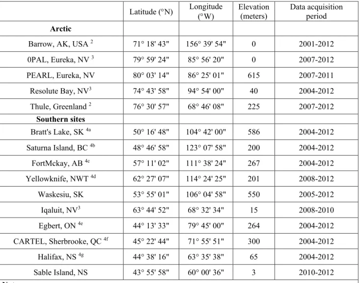
Table 1. AEROCAN/AERONET sites employed in this study. Latitude (N) Longitude (W) Elevation (meters) Data acquisition period Arctic

Barrow, AK, USA 2 _{71° 18' 43"} _{156° 39' 54"} ₀ _2001-2012

0PAL, Eureka, NV 3 _{79° 59' 24"} _{85° 56' 20"} ₀ _2007-2012 PEARL, Eureka, NV 80° 03' 14" 86° 25' 01" 615 2007-2011 Resolute Bay, NV3 _{74° 43' 58"} _{94° 54' 00"} ₄₀ _2004-2012 Thule, Greenland 2 _{76° 30' 57"} _{68° 46' 08"} ₂₂₅ _2007-2012 Southern sites Bratt's Lake, SK 4a _{50° 16' 48"} _{104° 42' 00"} ₅₈₆ _2004-2012 Saturna Island, BC 4b _{48° 46' 58"} _{123° 07' 58"} ₂₀₀ _2004-2012 FortMckay, AB 4c _{57° 11' 02"} _{111° 38' 24"} ₂₆₇ _2004-2012 Yellowknife, NWT 4d _{62° 27' 07"} _{114° 24' 25"} ₂₀₁ _2008-2012 Waskesiu, SK 53° 55' 01" 106° 04' 58" 550 2005-2012 Iqaluit, NV3 _{63° 44' 52"} _{68° 32' 34"} ₁₅ _2008-2010 Egbert, ON 4e _{44° 13' 33"} _{79° 45' 00"} ₂₆₄ _2004-2012 CARTEL, Sherbrooke, QC 4f _{45° 22' 44"} _{71° 55' 51"} ₃₀₀ _2004-2012 Halifax, NS 4g _{44° 38' 16"} _{63° 35' 38"} ₆₅ _2004-2012 Sable Island, NS 43° 55' 58" 60° 00' 36" 3 2010-2012 Notes

1. Sites have a nominal AOD sampling rate of 3 minutes (except for Barrow whose nominal rate is 15 minutes)

2. AERONET sites that are close to the AEROCAN regions 3. Nunavut, Canada. There was no data in 2005

4. "a" to "g"; the Canadian provinces of Saskatchewan, British Columbia, Alberta, North West Territories, Ontario, Québec, Nova Scotia

2.3.2 Ground-based retrievals of AOD

The basic AERONET instrument is the CIMEL sun photometer / sky radiometer manufactured by CIMEL Éléctronique. Different versions of the CIMEL exist (most notably the version that incorporates two additional NIR / SWIR channels at 1020 nm and 1640 nm and a version that permits nominal AOD sampling time intervals of 3

(25)

15

minutes as opposed to the older standard of 15 minutes). Except for Barrow with a nominal sampling time of 15 minutes, all instruments used in this study were versions incorporating the NIR/SWIR and 3-minute sample time capabilities. Solar extinction measurements acquired by the CIMEL instruments permit the retrieval of AOD spectra across eight channels (340, 380, 440, 550, 670, 870, 1020 and 1640 nm). The SDA is employed by AERONET to produce 𝜏_𝑓 and 𝜏_𝑐 estimates at a reference wavelength of 500 nm.

Combined solar extinction and sky radiance measurements are acquired at a significantly lesser (nominal) sampling frequency of once an hour and are employed in an AERONET inversion algorithm to extract columnar estimates of particle size distribution (PSD) and refractive index (Dubovik and King, 2000). The size distribution and refractive index can then be reprocessed to extract estimates of 𝜏_𝑓 and 𝜏_𝑐 across the 4 retrieval wavelengths (which can then be extrapolated to, for example, the standard SDA wavelength of 500 nm). The partitioning into 𝜏_𝑓 and 𝜏_𝑐 is accomplished by defining a cut-off bin size corresponding to the minimum of the retrieved volume PSD (i.e. a variable cut-off radius). The cut-off radius, the retrieved PSD and the refractive indices are then employed to extract 𝜏_𝑓 and 𝜏_𝑐.

The sampling rate is the key to the usage made of the different types of available retrievals: high frequency event-level studies and comparisons with lidar data are performed using 3-minute AOD spectra separated into 𝜏_𝑓 and 𝜏_𝑐 (see for example, Saha et al., 2010) while low frequency, climatological-scale analyses are carried out using the more comprehensive Dubovik inversions to extract 𝜏𝑓 and 𝜏𝑐. While some comparisons

have been made between the SDA and Dubovik retrievals of 𝜏𝑓 and 𝜏𝑐 (see O'Neill et al.,

2003) the Dubovik retrievals are much more of a climatological-scale standard than the SDA retrievals. We accordingly chose to use the Dubovik retrievals of 𝜏_𝑓 and 𝜏_𝑐 for the climatological-scale comparisons employed in this paper. The SDA retrievals were employed to investigate / identify specific events that were suspected of being artifactual in nature (statistical outlier events).

(26)

16

2.3.3 Level 1.5 versus Level 2.0 retrievals

Dubovik retrievals are available at Level 1.5 and Level 2 processing levels. The quality assurance criteria that define each level are given in Holben et al. (2006). In general, Level 1.5 retrievals are subject to certain QA protocols such as scan symmetry checks and requirements that (Level 2.0 extinction mode) AODs be acquired near the time of the almucantar scan (Level 2.0 extinction – mode AODs are defined at http://aeronet.gsfc.nasa.gov/new_web/data_description_AOD_V2.html ). The scan symmetry criteria along with the requirement for nearby Level 2.0 extinction-mode AODs amount to a form of cloud screening that is arguably more demanding than the extinction-mode AOD cloud-screening criteria that is incorporated in the Level 2.0 extinction-mode product. Level 2.0 retrievals are subject to additional QA criteria such as a maximum allowable sky radiance retrieval error (i.e. error residuals between the computed and measured almucantar sky radiance) and a minimal solar zenith angle. Table 2 compares Level 1.5 and Level 2.0 statistics for the three AOD components (𝜏_𝑎, 𝜏_𝑓, 𝜏_𝑐 at 500 nm) and the ensemble of all five Arctic sites across the 2009 - 2012 MYSP employed in this paper. In terms of total numbers, there are about a factor of 3 ½ times more Level 1.5 measurements than Level 2.0 measurements (5739 versus 1670). While Level 2.0 retrievals are the recommended option for users of AERONET retrieval products, we chose to use Level 1.5 retrievals because of the significantly greater number of points and the expected benefit of greater statistical robustness. At the same time, we monitored the Level 1.5 and Level 2.0 products at every averaging level in order to better understand any significant differences.

(27)

17

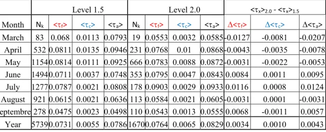
Table 2. Ensemble monthly means of Level 1.5 and Level 2.0 AOD components and the differences of two levels for 5 Arctic stations over the period of 2009-2012. Level 1.5 Level 2.0 <x>2.0 - <x>1.5 Month Nk <f> <c> <a> Nk <f> <c> <a> <f> <c> <a> March 83 0.068 0.0113 0.0793 19 0.0553 0.0032 0.0585 -0.0127 -0.0081 -0.0207 April 532 0.0811 0.0135 0.0946 231 0.0768 0.01 0.0868 -0.0043 -0.0035 -0.0078 May 1154 0.0814 0.0111 0.0925 666 0.0783 0.0088 0.0872 -0.0031 -0.0022 -0.0053 June 1494 0.0711 0.0037 0.0748 353 0.0795 0.0047 0.0843 0.0084 0.0011 0.0095 July 1277 0.0787 0.0021 0.0808 178 0.0903 0.0029 0.0933 0.0116 0.0008 0.0124 August 921 0.0615 0.0021 0.0636 113 0.0584 0.0021 0.0605 -0.0031 0.0001 -0.0031 Septembre 278 0.0475 0.0023 0.0498 110 0.0543 0.0013 0.0555 0.0068 -0.0011 0.0057 Year 5739 0.0731 0.0055 0.0786 1670 0.0764 0.0065 0.0829 0.0034 0.0010 0.0043

With respect to Table 2, the most notable differences occur in the months of March, June and July with values of < 𝜏𝑎,2.0 > − < 𝜏𝑎,1.5 > = −.021, 0.010 and 0.012

respectively and an average of − 0.003 for the rest of the months (numbers that can be contextualized by corresponding Level 1.5 standard deviations of 0.041, 0.065, and 0.059). The month of March has only 83 and 19 measurements respectively across the Level 1.5 and 2.0 ensembles: in such cases of near marginal statistics associated with very low numbers of retrievals (always problematic during the Polar dusk months of March and September), our feeling is that Level 2.0 measurements are much more likely to be subject to the vagaries of unrepresentative measurements than Level 1.5 data. The ensemble statistics for the months of June and July are subject to large 𝜏𝑓 variations (the

standard deviations are large for both Level 1.5 and Level 2.0 data): this is likely due to seasonal smoke events (see the station by station fine mode discussion below).

2.3.4 GEOS-Chem simulations

The model that we employed for our comparisons was Version 9-01-03 of the GEOS-Chem global chemical transport model (GC). It is driven by GEOS-5 assimilated meteorological ﬁelds from the NASA Goddard Modelling and Assimilation Ofﬁce (GMAO). We used a 15-minute time step for transport and a 60-minute time step for chemistry and emissions, a latitude / longitude grid size of 2 by 2.5 (approximately 220 km x 50 km at the high Arctic latitude of 0PAL and PEARL and 220 km x 90 km at

(28)

18

Barrow) 47 vertical levels up to 0.01 hPa. The temporal resolution of the GC AODs which we employed in our analysis was 6 hours.

An overview of AOD physics and chemistry in GC is given in Park et al., (2004). We divided the simulated AODs into their fine and coarse mode components (𝜏_{𝑓,𝐺𝐶} and 𝜏_{𝑐,𝐺𝐶}) using the species by species segregation provided by GC. The species are fine mode organic carbon (OC), sulfate (SO4) and black carbon (BC) along with fine and coarse mode sea-salt (SS) as well as fine and coarse mode mineral dust). Accordingly;

𝜏_{𝑐,𝐺𝐶} = 𝜏_{𝑐,𝐺𝐶,𝑆𝑆} + 𝜏_{𝑐,𝐺𝐶,𝑑𝑢𝑠𝑡} (4𝑎)

𝜏_{𝑓,𝐺𝐶} = 𝜏_{𝑓,𝐺𝐶,𝑆𝑂4} + 𝜏_{𝑓,𝐺𝐶,𝐵𝐶} + 𝜏_{𝑓,𝐺𝐶,𝑂𝐶} + 𝜏_{𝑓,𝐺𝐶,𝑆𝑆} + 𝜏_{𝑓,𝐺𝐶,𝑑𝑢𝑠𝑡} (4𝑏) All AODs are calculated at 550 nm using RH-dependent aerosol optical properties (see Martin et al., 2003 for an overview of the optical processing employed for GC aerosols). The dry-mass particle size distributions of all components except dust are represented by lognormal distributions implicitly partitioned into fine and coarse mode components according to their effective radius (http://wiki.seas.harvard.edu/geos-chem/index.php/Aerosol_optical_properties). Dust is represented by a gamma distribution divided into 7 size bins (ibid): in this paper, we defined the fine and coarse mode cut-off radius for dust to be at 1.0 µm (meaning 4 fine-mode bins and 3 coarse-mode bins).

Emission sources in GEOS-Chem are generally dynamic with ties to temporally varying empirical indictors of emission strength (see "Aerosol emissions" on the GEOS-Chem Wiki site at http://wiki.seas.harvard.edu/geos-chem/index.php/Aerosol_emissions). Biomass burning emissions, for example, employ GFED3 emission estimates which are, in turn, based on MODIS-Terra and MODIS-Aqua fire counts acquired over sampling intervals of 3 hours. As another relevant example, dust emissions are driven dynamically by mobilization schemes that employ analysed wind fields.

2.3.5 AOD differences due to small changes in the reference

wavelength: GC versus AERONET retrievals

(29)

19

past calculations and those of others, we chose a reference wavelength of 500 nm for the AERONET retrievals. The expected negative bias of the 550 nm AODs relative to 500 nm AODs is generally small compared to the retrieval standard deviations (<~ 20% of the ensemble monthly standard deviations for the fine, coarse and total components)

2.4. Results and discussions for the Canadian Arctic

2.4.1 Analysis of lognormal versus normal representations

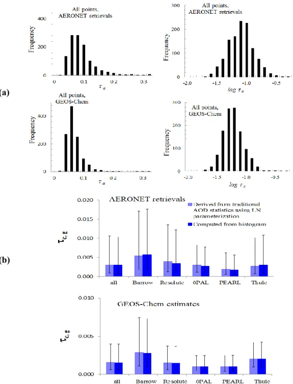
Figure 2 (a) shows normal and lognormal histogram representations of the total AOD (𝜏_𝑎) for both the AERONET retrievals (Level 1.5) and GEOS-Chem simulations respectively (for all points of the MYSP). In keeping with the conclusions of O’Neill et al. (2000) the top two AERONET histograms confirm that a lognormal representation is more appropriate for Arctic data (the histogram on the logarithmic scale looks more like a normal distribution, while the histogram on the linear scale shows a typical asymmetric, positively skewed, form). The bottom two histograms of Figure 2 (a) illustrate that the GC modelled histograms show the same general characteristics as their measured analogues. This general agreement in the form of measured and modelled histograms (also a characteristic of the fine and coarse modes) is a verification of the real-world simulation capability of the model: an element of model evaluation that we have not noted in the literature.

(30)

20

Figure 2. Normal and log-normal fit comparisons for AERONET and GC AOD histograms (a) Linear and lognormal histograms (left and right-hand graphs, respectively)

for AERONET at λ = 500 nm and GC at λ = 550 nm (top and bottom rows respectively), (b) An example of how to employ the traditional means of reporting sun photometry

AOD statistics (linear mean and standard deviation) to extract parameters that are representative of the lognormal distribution. In this illustration the linear mean and

standard deviation are used to estimate the geometric mean of the histogram by calculating the latter from the lognormal parameterization (equations (2) and (3)).

(a)

(31)

21

Figure 2 (b) illustrates the estimation of the geometric mean of an AOD histogram, given the lognormal parameterization and the arithmetic mean statistics (given equation (3)). For this particular coarse mode example (as a function of station for all points during the MYSP) we compare the computed geometric mean from equation (2) with the actual geometric mean of the data histogram for both the AERONET retrievals and GC simulations (the disparity between the optical depth amplitudes of the measured and modelled results will be discussed below). The results show that the geometric mean values from equation (2) are close to the geometric means from the data histograms for both the AERONET retrievals and the GC simulations (less than 20% and 5% difference for measurements and models respectively): this is really just an illustrative confirmation that measured and modelled AOD histograms are better represented by a lognormal distribution. In terms of the overwhelmingly common tendency to report AOD statistics in terms of arithmetic statistics, this result indicates that geometric statistics can be readily retrieved by future analysts and modellers from the arithmetic statistics (providing the arithmetic statistics include at least the arithmetic mean and standard deviation).

2.4.2 General AOD statistics for the retrievals

― General considerations

For various reasons, we chose the climatological sampling period (MYSP) of 2009 - 2012 for the analyses presented in this paper. At the same time, we regularly monitored the robustness of the 2009-2012 statistics compared to the statistics of a longer, 2007 - 2012 MYSP. All months with 10 or fewer retrievals for any given station across our MYSP were excluded from the analyses in order to maintain a rudimentary degree of statistical significance and robustness in the worst cases of sparse data (this eliminated the month of March for PEARL, April for 0PAL and all of the October retrievals).

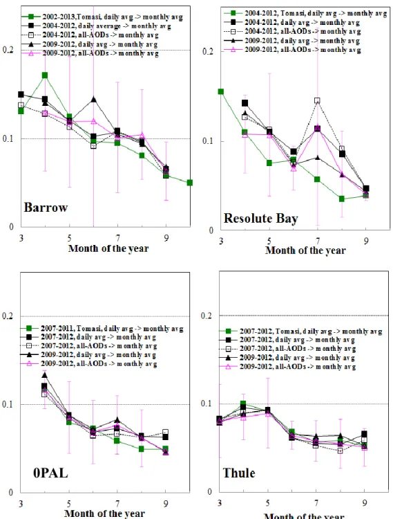
Figure 3 shows a sensitivity study that includes a variety of types of 500 nm AOD monthly averages referenced to the (green colored) monthly averages of Tomasi et al. (2015) for the four sites that were in common between our two studies (the Tomasi study is the only recent sun photometry multi-year analysis that includes AERONET stations common to our own). The solid symbols represent monthly averages of daily averaged

(32)

22

retrievals while the open symbols represent monthly averages employing all individual retrievals (without pre-averaging). The open-symbolled curve in purple (and its standard deviation error bars) represents our monthly averaging scheme over our selected MYSP. The comparisons with Tomasi are not identical even when the MYSP and the averaging scheme are identical because they employed AOD retrievals (solar extinction data) for their statistical analysis while our analysis comes from AODs processed through the AERONET Dubovik retrieval. This brings up an interesting predicament: their analysis nominally employs about a factor of five more AODs (and thus is nominally more statistically sound) than our analysis while one could argue, that the retrievals are better filtered than the AODs (both in terms of cloud screening and in terms of the physical soundness of the derived products; see Holben et al., 2006 for a general discussion of Dubovik retrieval filtering).

(33)

23

Figure 3. Comparison between various types of monthly averages (black and purple) and the monthly averages (green) of Tomasi et al. (2015). The Tomasi AOD averages represent Level 2.0 extinction data. The purple curve shows the averages for the MYSP.

The error bars are standard deviations.

As can be seen in Figure 3, the agreement (of any of the curves) with the station by station, multi-year Arctic AOD analysis of Tomasi (2015) is rather marginal for the two western stations of Barrow and Resolute Bay, affected as they are by intermittent,

(34)

24

amplitude smoke events (see the fine mode station by station analysis below for further discussions). Indeed, the results can be rather precarious with large changes between the various types of averaging schemes and with variances that are considerably larger than the eastern station variances (as represented by the standard deviations of our chosen averaging scheme). In one particularly egregious example, the removal of two super-unity 𝜏_𝑓 days of data from Barrow's "daily avg -> monthly avg" scheme for June (black triangles in Figure 3) yielded a reduction in < 𝜏_𝑓 > and 𝜎(𝜏_𝑓) of 0.046 and 0.187 respectively for the month of June (in effect the process of daily averaging before monthly averaging enhanced the statistical weight of those two days2_{). This level of} precariousness appears to be damped down by averaging over a longer MYSP of 2004 to 2012. However, such was not the case for the highly variable month of July in the Resolute Bay results: the same increase in the MYSP duration produced even greater departures from the Tomasi results. If we leave aside the case of July in Resolute Bay the RMSD values relative to the Tomasi results for our chosen MYSP and all 4 stations (the purple vs the green curves) vary from <~ 0.02 for the western stations to <~ 0.01 for the eastern stations (values that are all <~ the standard deviations of our chosen MYSP).

― Seasonal variations of the total AOD

Figure 4 shows the 〈𝜏_𝑎〉 monthly mean variation for the total MYSP data ensembles of the 5 Arctic and 10 southern stations (the error bars represent the standard deviations as defined in the section on averaging and standard deviation statistics). In general, one can note the larger (if not always significantly larger) southern AODs and a peaking of the Arctic AODs in April (~ 0.10) with a decrease in the summer to fall period (~ 0.05 in September) while the southern station ensemble shows AOD (500 nm) peaking during the late summer (c.f. Holben et al., 2000, for general multi-year statistics of southern stations). The 8-station, (1999 - 2011) Arctic (AERONET) averages of Breider et al. (2014) and the (2004 - 2006) Alert results of Hardenberg et al. (2012) show a broadly similar type of (550 nm AOD) behaviour as do the 500 nm results of Tomasi et al.

2_{June 12, 13, 2010 for which only 3 Level 1.5 retrievals were actually archived. The "all-AODs->monthly} averaging" (pink) case placed  a factor of 3 less weight on those 3 measurements for the month of June 2010 (this is reflected in the lower pink triangle in the June, Barrow case of Figure 3.

(35)

25

(2015). Eck et al. (2009) show a similar (500 nm) AOD trend at Barrow for a 1999 - 2008 MYSP (with infrequent, large amplitude excursions due to smoke) while the interior (Boreal forest) Alaskan site of Bonanza Creek showed a smoke dominated peak in August for seasonal statistics across a MYSP of 1994 to 2008.

Figure 4. 〈 τa 〉 (averaged over the 2009 to 2112 MYSP) as a function of month for the Arctic stations compared with the analogous averages for the 10 southern stations. The

error bars are standard deviations

2.4.3 Comparisons with GC

― Component AODs averaged over all stations

Retrieved and modelled seasonal plots of monthly averaged component AODs (〈𝜏_𝑓〉, 〈𝜏_𝑐〉 and 〈𝜏_𝑎〉 for all the Arctic stations across our chosen MYSP of 2009 to 2012 are shown in Fig. 5. Both retrieved and modelled plots of 〈𝜏_𝑓〉 indicate a peak in the April/May period and in July (the latter peaking being not unrelated to the above comparisons with the Tomasi reference). The GC estimations are systematically less than the retrievals but the differences of <~ 0.03 are usually within the retrieval standard deviations.

Peaking of 〈𝜏_𝑐〉 in April / May can be observed for both the retrievals and GC, with a significant amplitude disparity. GC results are relatively independent of the MYSP while retrieved 〈𝜏𝑓〉 and 〈𝜏𝑐〉 values are also fairly robust: the RMSD values of 〈𝜏𝑓〉2007−2012−

(36)

26

〈𝜏_𝑓〉_2009−2012 and 〈𝜏_𝑐〉_2007−2012− 〈𝜏_𝑐〉_2009−2012 for the 2007 - 2012 MYSP relative to the 2009 - 2012 MYSP were computed to be 0.0035 and 0.0032 respectively (values that are respectively much smaller than and less than or of the order of the standard deviation error bars seen in Figure 5).

Figure 5. 〈 τf 〉 , 〈 τc 〉 and 〈 τa 〉 (monthly averages over the 2009 to 2112 MYSP) and modelled values (〈 τf,GC〉 ,〈 τc,GC〉 and 〈 τa,GC 〉 ) as a function of month. The error

(37)

27

― Individual stations

 Linear and logarithmic regressions of modelled AOD versus AERONET AODs

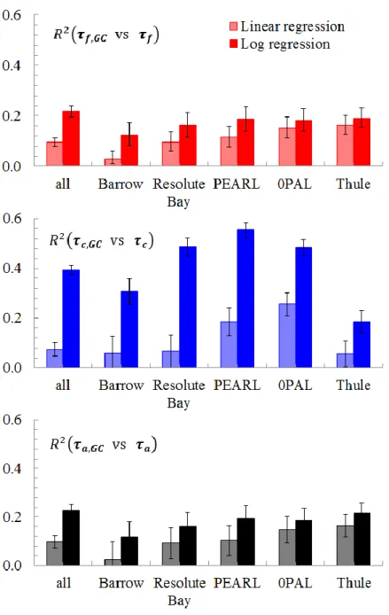
Figure 6 shows the GC versus AERONET coefficient of determination (R2_{) computations} for daily averaged 𝜏𝑎, 𝜏𝑓, and 𝜏𝑐 values as a function of the measurement station (as

well as the combination of all station data) over the total MYSP. The plot includes a comparison of R2_{for linear regressions (both modelled and AERONET AODs in linear} space) as well as logarithmic regressions (both modelled and AERONET AODs in log space). The error bars correspond to one standard deviation of the Fisher's z transformation distribution (see, for example, Siegel, 1961). One can observe that the logarithmic regression is always characterized by a higher R2_{value but that the value is} not always significantly higher in the case of 𝜏𝑓 𝑎𝑛𝑑 𝜏𝑎 (notably for the eastern Arctic

stations). In the case of 𝜏𝑐, the values show a significant improvement over the linear

regressions for the "all" (stations) case and for each individual station. A superiority of R2 values in log-space compared to R2_{values in linear space, for lognormally distributed} data frequencies has been noted, for example, by Zerovnik et al. (2013)3 _{where the degree} of superiority was shown to vary with the strength of correlation between the independent and dependent variables and the COV (coefficient of variation) of the two variables , The results of Figure 6 are, in fact, further confirmation that both the retrieved and modelled AOD distributions are lognormal.

3_{Specifically, their Figure 3 where their lognormal coefficient C}(ln)_{is the coefficient of correlation for the} linear space where the data probability distribution appears as lognormal while C(n)_{is the coefficient of} correlation for the log space where the data probability distribution appears as normal.

(38)

28

Figure 6. Coefficient of determination between modelled and retrieved daily AOD means for the ensemble of all sites ("all") and for individual sites. The error bars are the standard deviations corresponding to one standard deviation of Fisher's z transformation

distribution (see Siegel, 1961, for example).

The superiority of R2_{values in log-space should be at its greatest when the COV is} largest (ibid): this is the case for (retrieved and simulated) coarse-mode COVs which were >~ 1 while fine and coarse-mode COVs where <~ 1. The significant logarithmic

(39)

29

correlation is likely an indication that even though 〈𝜏_𝑐〉 and 〈𝜏_{𝑐,𝐺𝐶}〉 are <~ the standard sunphotometer AOD error4_{, their estimation / retrieval significance can be well below} that nominal error. This means that the GC estimates can still be physically significant even though, for example, the simulated source strengths might be substantially underestimated. On the retrieval side this means that the estimation of 𝜏_𝑐 is essentially a small fraction of 𝜏𝑎 that depends (mostly) on the spectral shape of the latter: the influence

of this spectral shape scales down to the small values of 𝜏_𝑐 that result from the retrievals.  Fine mode seasonal variations

Figure 7 shows 〈𝜏_𝑓〉 and 〈𝜏_{𝑓,𝐺𝐶}〉 monthly average values for our chosen 2009-2012 MYSP in terms of the individual stations. The first thing we would note is the coherency of the PEARL and 0PAL retrievals. The simple average of the monthly average differences (< 𝜏_𝑓>_{0𝑃𝐴𝐿} − < 𝜏_𝑓 >_{𝑃𝐸𝐴𝑅𝐿}) for the 0PAL and PEARL bar graphs of Figure 7 is 0.0013: that this is a very small positive number5_{well below the expected errors of CIMEL} AODs is fortuitous. However, the fact that it is small in general does permit us to exploit the very useful redundancy afforded by the near co-location of the two instruments.

4_{for newly calibrated instruments these are typically < 0.01 for λ > 440nm and < 0.02 for shorter} wavelengths (Holben et al., 1998).

5_{As expected for an 0PAL CIMEL instrument which sees a moderately thicker atmosphere from its} sea-level location.

(40)

30

Figure 7. 〈τf 〉 Fine mode monthly averages over the MYSP for all 5 Arctic sites. The error bars

are the standard deviations.

Resolute Bay, as well as 0PAL and PEARL to a moderate degree, show 〈𝜏_𝑓〉 peaking in July while the Resolute Bay standard deviation is very large (COV ~ 1.5) in keeping with the general averaging comments made above about the variability of AODs during this month (the fact that both 0PAL and PEARL show a weak peak is an example of the

(41)

31

potential values of the redundancy mentioned in the previous paragraph). That this AOD variability is largely in the fine mode and that it is likely smoke, is in keeping with our SDA investigations using individual events during the MYSP and, in general with our SDA / lidar experience that smoke is a common fine mode phenomenon in the Arctic (see Saha et al., 2010 for example). Barrow displays June peaking with a large standard deviation (also in keeping with general averaging comments made above). The fine mode contribution of Resolute Bay is largely responsible for the July peaking seen in Figure 3. That peaking is, at best, marginally evident in the GC simulations and the OC contribution to that marginal peaking is roughly shared between fine mode sea-salt and fine mode sulphates (in other words there is no GC evidence for strong seasonal smoke influence at Resolute Bay during the month of July).

Excluding the peaking of the retrievals in July and the Barrow peak in June (as we did for the Tomasi comparison above and as we noted for the all-station case), one can generally observe a broad and decreasing, spring to fall 〈𝜏𝑓〉 trend displayed by all the stations with

a peak in April / May. The 〈𝜏_{𝑓,𝐺𝐶}〉 curves show a broad and weak peak in April / May with a moderate July inflection: this behaviour results from a combination of a strong biomass-burning OC peak in May and a decreasing sulphate trend from an Arctic haze peak in February, both of which decrease until June where they tend to flatten out. The average GC underestimate relative to the retrievals, for all the sites is 0.0132 (a general figure, without excluding any months).

 Coarse mode seasonal variations

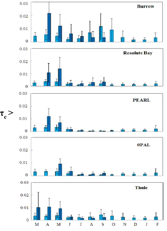
Coarse mode, 〈𝜏𝑐〉 and 〈𝜏𝑐,𝐺𝐶〉 monthly average results are shown in Figure 8 for each

station. We found infrequent but strong 𝜏_𝑐 outlier excursions in the individual retrieval results with a significant effect on the monthly means and standard deviations (<~ 1 to 10 outlier excursions for ~ 20 to 400 retrievals in a given monthly bin over the MYSP). A 3σ outlier exclusion filter was accordingly applied to the coarse mode, individual station retrievals and these are the results seen in Figure 8. Investigations of a few trial cases using the SDA applied to high-frequency solar extinction data suggested that these strong 𝜏_𝑐 excursions were due to temporally and spatially homogeneous clouds whose 𝜏_𝑐 contributions had not been eliminated by the cloud screening impacts of the Level 1.5

(42)

32

retrieval QA protocols defined in Holben et al. (2006). We note that no appeal could be made to Level 2.0 retrievals since the number of retrievals in a given monthly bin was, more often than not, <~ 10.

Figure 8. 〈τc〉 Coarse mode monthly averages over the MYSP for all 5 Arctic sites. The error bars are the standard deviations.

The AERONET retrievals of Figure 8 indicate < 𝜏𝑐 > peaking in April / May for all

stations while a degree of weak < 𝜏_𝑐 > peaking can be observed in the August /

Comparisons of an aerosol transport model with a 4-year analysis of summer aerosol optical depth retrievals over the Canadian Arctic