Public bus transport demand elasticities in India

Public bus transport demand elasticities in India

Kaushik Deb, TERI University, New Delhi, India Massimo Filippini, ETH, Zurich, Switzerland

Address for Correspondence

Kaushik Deb is an Associate Professor at TERI University, Plot No. 10 Institutional Area, Vasant Kunj, New Delhi - 110 070, India (kdeb@teriuniversity.ac.in)

Massimo Filippini is a Professor of Economics at the Department of Management, Technology, and Economics, ETH, Zurich, Switzerland and at the Università della Svizzera Italiana, Lugano, Switzerland.

Abstract

A number of static and dynamic specifications of a log linear demand function for public transport are estimated using aggregate panel data for 22 Indian states over the period 1990 to 2001. Demand has been defined as total passenger kilometers to capture actual market transactions, while the regressors include public transit fare, per capita income, service

quality, and other demographic and social variables. In all cases, transit demand is significant and inelastic with respect to the fare. Service quality, approximated by the density of the coverage of the transport service, seems to be an important variable that affects demand. Although this is an important explanatory variable, service quality improvements should be preceded by a cost benefit analysis. Finally, social and demographic variables highlight the complex nature of public bus transit demand in India.

Keywords

Demand Elasticities, Dynamic Panel Data, Bus Transport, India

JEL Classification

1.0 Introduction

Rapid economic development exerts pressure on all infrastructure services vital for economic efficiency and social sustainability, particularly transport infrastructure. In India, sustaining this increase in economic productivity is contingent on meeting the mobility demand that such economic growth creates, and hence on optimally utilizing existing

infrastructure (Justus (1998); Gowda (1999)). In addition, transport accounts for a substantial and growing proportion of air pollution in Indian cities, contributes significantly to

greenhouse gas emissions, and is a major consumer of energy (Ramanathan and Parikh (1999)). Transport is also the largest contributor to noise pollution, and has substantial safety and waste management concerns (Singh (2000)). Finally, access to transport services is considered critical for addressing equity concerns by facilitating access to primary education and employment generation facilities. Transport infrastructure is also important for integrating rural communities in the socioeconomic structure of the nation.

This calls for a greater share of public transport in meeting mobility needs. Not only is an efficient public bus system important for meeting the mobility needs in this rapidly

growing economy, but a higher share of bus transport would also reduce pollution, both local and global, and energy demand. Hence, it is incumbent on governments in developing

countries to institute appropriate policy initiatives to increase the share of public transport. Such interventions must be informed by research that identifies factors influencing the demand for public transport. The most common method for characterizing the influence of such variables is by estimating the elasticity of demand with respect to each of these variables. To this end, this paper estimates the elasticity of demand at the state level with respect to price, income, and service quality. All states with public bus transport in India are included in this study.

There are two major types of empirical transit demand studies, namely, those derived from the Random Utility Theory that analyze the choice of a transport mode (Winston (1983); Oum (1989)), and those derived from consumer utility maximization that analyze continuous consumption patterns. Demand analysis in the case of a continuous variable, in turn, follows one of two approaches. The first approach estimates a system of equations simultaneously for several commodities or commodity groups. The second focuses only on one commodity, or a commodity group, and hence essentially estimates the demand in a single market. In either case, with a complete systems approach that is theoretically more consistent, a more comprehensive dataset is required that includes demand for, or expenditures on, all

commodity groups. In the absence of such an extensive dataset, equations are specified in a more ad hoc manner including cross–commodity influences from only close substitutes and complements (Thomas (1987)).

This research uses an unbalanced aggregate panel dataset between 1990/91 and 2000/01 for 22 large states in India to assess the price and income effects on public bus transport demand. Here, direct price elasticities can be obtained after estimating an ad hoc aggregate single equation demand model. The current research is possibly one of few studies that use panel data for the estimation of the Indian bus transport demand.

The paper is organized as follows. The next section briefly describes the public road transport sector in India. Section 3.0 discusses the relevant literature on number, timing, and spatial distribution of trips by mode in estimating travel demand, all of which are infinitely faceted and hence can result in a large variety of alternatives for each consumer, making travel demand modeling complex (Jovicic and Hansen (2003)). The specification used in this research is given in section 4.0. The estimation process and the data used are given in section 5.0. Section 6.0 presents the results of the analysis and discusses the implications therein, and finally, section 7.0 concludes.

2.0 Public bus transport in India

Public bus transport in India is overwhelmingly provided by government owned bus companies. Even though the private sector owns more buses than the government, privately owned buses are rarely allowed to operate as public transport and are generally put to use in servicing schools and other educational institutions, tourists, etc. on contract basis. The participation of the government in road transport commenced in 1950 and since then government owned bus companies have been formed in every state (Gandhi (1999)). These firms are called State Road Transport Undertakings. At present, there are 52 government owned bus companies in the country. Out of the 52 firms, 14 operate exclusively in the urban areas, 8 only in rural areas, and the remaining 30 provide services in both urban and rural areas. All bus companies are regulated as per the Road Transport Corporations Act (1950) and the Motor Vehicles Act (1988) by the state government (Deb (2003)).

In the road transport sector in India, liberalization of the automobile industry in parallel to a rapid increase in per capita incomes has led to a shift towards personal vehicles. The share of public transport, on the other hand, has declined over time. The economy is now being constrained by the increasing number of vehicles causing congestion, and thus slower speeds on roads. Transport infrastructure is recognized as being the critical constraint here (Ramanathan and Parikh (1999)). Efficient and optimal utilization of the available transport infrastructure would require meeting mobility needs through a greater share of public

transport (Planning Commission (2002)). More importantly, since most passenger transport in India is road based, the share of public bus transport should be increased (Ramanathan and Parikh (1999)). This calls for an increase in the capacity of the government owned public bus companies in India (Singh (2005)). In addition, given that access to public transport is not universal in India, an improvement in access to public transport is an important attribute of service quality.

3.0 Literature review

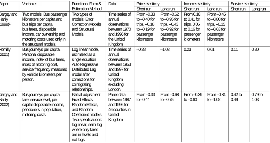
The literature has been reviewed in the context of the framework suggested by Berechman (1993) assessing the impact that different specifications and estimation approaches have on demand elasticities. The focus in this review is on aggregate demand estimations as attempted in this paper, ignoring the extensive literature estimating discrete modal choices. A summary of recent studies using either panel data or those estimating aggregate demand functions is presented in Table 1.

Most travel demand models use the number of trips or passengers as the dependent variable (Hanly and Dargay (1999); Romilly (2001); Dargay and Hanly (2002)). Dargay and Hanly (1999) is the only study in the literature review undertaken that uses passenger

kilometers as the measure of demand for their aggregate national analysis of travel demand. However, using only the number of trips or passengers as a measure of travel demand ignores an important characteristic of demand, the length of each trip. This is clearly an important parameter that also reflects the motivation for the supply and pricing of public transit services. The objective of this research is to identify factors that influence public bus transit demand from the perspective of the bus transport industry. Hence, the definition of demand needs to reflect actual market transactions. Using passenger kilometers as a demand measure allows transit demand to be related to a supply measure and can then be used to analyze public transit markets, as is the objective of this research. The two measures of transit demand, the number of passengers and passenger kilometers, are highly correlated in the dataset used in this analysis, with a correlation of over 90%. Hence, passenger kilometers are taken as the output measure. Moreover, a measure of the extent of operation, proxied by the population of the state that the firm is based in, could be suitably used as an indicator of market size.

In terms of independent variables, studies cited in the literature review have included monetary variables such as the price of the service, prices of available alternatives, and wealth

or income levels as well as non–monetary variables such as quality and demographic or cultural attributes such as occupation, lifestyle, age, and gender (Wabe (1969); Kemp (1973)). Matas (2004) uses the level of suburbanization and employment levels to explain demand changes in Madrid during 1979–2001. The empirical estimation of the effect of these variables on transit demand is not always straightforward since many of them are highly correlated with income or other socioeconomic variables.

A public transit demand model should include some variables representing the quality of the service. Some studies use output measures such as vehicle kilometers as service quality measures (Goodwin and Williams (1985); Fitzroy and Smith (1993); Balcombe, Mackett et al. (2004)). Such measures, however, result in an identification problem between the variable defining demand, and the variable defining service quality. In addition, service quality changes due to changes in capacity, such as larger buses resulting in more seat kilometers, would be ignored in such a measure (Balcombe, Mackett et al. (2004)). Other aggregate service quality measures use the ratio of network length to area size or population as a proxy of access to transit services to avoid such identification issues (Romilly (2001); Dargay and Hanly (2002)). Bresson, Dargay et al. (2003) estimate a log linear specification with income, price, and network density as variables for quality. FitzRoy and Smith (1997) argue that journey time is an important quality parameter and use average frequency and route density as proxies. In the context of a developing country such as India, Maunder (1986) and Palmner, Astrop et al. (1996) highlight the importance of access to public transport routes as a measure of public transport quality.

There are various functional forms that have been used in the literature to estimate aggregate transit demand, namely, linear functions, semi–log or log linear, and generalized non–linear models (de Rus (1990); Appelbaum and Berechman (1991)). The most common functional form used is the log linear (Romilly (2001)). Only a handful studies have estimated

a semi–log functional form where only transit price is included in levels and all other explanatory variables are in logs (Dargay and Hanly (2002); Bresson, Dargay et al. (2003)). Another advantage of the log-linear functional form is that the coefficients can be readily interpreted as elasticities. Finally, the log linear form also allows for non–linear interactions between demand and the various parameters, hence capturing more complex relationships than simple linear effects (Oum (1989); Clements and Selvanathan (1994)).

A small number of studies have used panel data that combine cross sectional and time series data. The current research is possibly one of the few studies estimating a static and dynamic travel demand specification using aggregate data for developing countries. Unlike other studies that estimate demand functions for India using datasets comprising a limited number of firms or cities, this study uses panel data from almost all states in India, including both urban and rural areas, and hence provides a comprehensive analysis of public transit demand in India. In terms of methodology, this research compares the results from several econometric approaches for static and dynamic demand models detailed in section 4.

4.0 Model specification

The model specification presented in this section is based on the review of the literature presented above and the issues discussed therein. Since the study assesses public bus transit price elasticities in the context of actual market transactions, passenger kilometers have been taken as the demand measure (pkm). Several variables have been selected as explanatory variables. Public bus transit fares (Public transit fare) and per capita income (

Per capita income) are the monetary variables. Service quality is characterized by the density of coverage (Densiy of coverage). The total population (population) of the state is included to isolate the effect of size of the market. The demographic and socioeconomic variables in the model are the proportion of population in the labour force (Labor force participation) and

literacy rate (literacy)1. Unfortunately, data on the prices of substitutes and complements are not available in this study. The only significant transport service here is personal vehicle usage. The impact of changes in personal vehicle usage can be approximated using another socioeconomic variable, per capita private vehicle ownership (Vehicles per person).

From the studies reviewed in Table 1, the functional forms most commonly used in the literature are log linear and semi–log. Since the log linear form is easily interpretable, and simple for computing elasticities, the log linear function has been estimated2. The

demographic variables are already in percentages. These have not been converted into logs and are included as reported. In this case, the coefficients can be readily interpreted as elasticities. Thus, the static model is the following,





























Vehicles per person population

Public transit fare Per capita income Densiy of erage Labor force participation

literacy                  (1) The dynamic structure of demand has been captured using a partial adjustment model.

This implies that given an optimum, but unobservable, level of transit demand,pkm , demand *

only gradually converges towards the optimum level between any two periods. Hence,

*

, 1 , 1

Lnpkm_it Lnpkm_{i t} (Lnpkm Lnpkm_{i t} ) _it (2)

1

The proportion of population living in urban areas and the sex ratio were also included in early specifications on the model. However, these variables did not significantly improve the goodness of fit. In addition, in terms of the elasticities obtained for the key variables of interest, these were not found to have any significant influence.

2

The elasticities obtained from using the log linear and the semi–log functional forms were compared and found to be similar.

where





 is random disturbance (Kmenta (1978)). Substitutingpkm in the dynamic adjustment *

equation gives:





























Vehicles per person population

pkm Public transit fare Per capita income Densiy of erage Labor force participation

literacy pkm                           _1 _it (3)

where_i _i and_it _it  . This dynamic specification is estimated. _it This is possibly one of the few studies estimating public bus transit demand in developing countries. The specification being used also attempts to capture actual market transactions to relate these with firm behaviour using passenger kilometers as a measure of demand. In addition, using density of coverage provides a proxy indicator of service quality in terms of access to the transit network, and hence avoids simultaneity with the measure of demand and output. Finally, the use of demographic and social characteristics is expected to reveal the import of such non–monetary variables in the context of a developing country.

5.0 Data and econometric approaches

An unbalanced panel of 22 states in India between 1990/91 and 2000/01 has been used in the analysis with 206 observations. The panel ranges from 21 states in 1993/94 to 16 in 1997/98. This data set is characterized by a relatively small number of cross-sectional units and a relatively long time period. Data on public bus transit demand for the entire state, including both urban and rural areas, has been taken from CIRT (Various years)3. Public bus transit fares have been estimated as the ratio between traffic revenue and total demand, with

3

For the six states with more than one operator, data has been summed across all the operators to obtain state level aggregates.

the information obtained from CIRT (Various years). Thus, non–traffic revenue, such as advertising revenue or interest accrued, has been excluded from the definition of public transit fares. Unfortunately, user costs and external costs are not available for this study and hence only public bus transit fares are included. Hence, the price elasticities obtained are only for public bus transit fares and not generalized transportation costs for the public bus users as in Mohring (1970).

Density of coverage has been estimated as the ratio between vehicle kilometers

reported in CIRT (Various years) and the area of each state. Demographic and social variables have been obtained from Census of India 2001 (2001). The per capita income series is based on total State Domestic Product reported in EPWRF (2003) and population totals from Census of India 2001 (2001). Private vehicles in the analysis have been defined as cars, two–

wheelers, and jeeps, with the data from MTS (Various Issues). This has been divided by the population of each state to obtain the per capita private vehicle ownership. The two monetary variables, namely public bus transit fares and per capita incomes, have both been deflated to 1989/91 prices using the Wholesale Price Index for All Commodities reported by the

Government of India (2005) to carry out the estimations in terms of real values4.

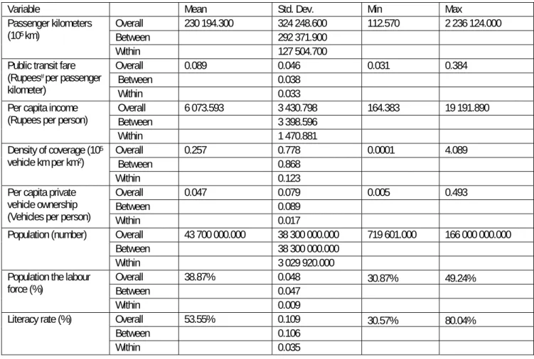
Table 2 describes the dataset and the variables used in the analysis. Each observation

of each variable, x ,has also been decomposed into two separate series of between _it

observations it i _t x x T  _   





x x x

I

 _{ } 

 





4

The price index data in India is available in the form of a Wholesale Price Index and four Consumer Price Index series. The only aggregate price index available in India is the Wholesale Price Index since it is not possible to aggregate the four Consumer Price Indices into one composite index. However, it may be noted that tests show that the trend-level CPI lags is strongly correlated with the WPI.

(STATA (2005)). For most variables, the overall variation in the dataset comes from the Between Variation. In addition, there is a large variation in the dataset for most variables as can be observed from the minimum and maximum values. Hence, it is important to include a variable that reflects the size differences between states. This size effect is captured by using the total population of each state.

With regard to the choice of econometric technique, it should be noted that in the econometric literature there are various panel data models that take into account unobserved heterogeneity across units. Moreover, we can distinguish between static and dynamic econometric approaches5. In this paper we estimated the static version of the demand model (1) using the two classical panel data estimators, the Fixed effects (FE) and the Random effects estimators (RE). Moreover, to account for possible endogeneity of the price and quality variables, we estimate the static models using the lag variable for price and quality6.

In estimating the dynamic panel data model (3), FE or a RE is not appropriate because the inclusion of a lagged dependent variable in the explanatory variables violates the strict exogeneity assumption. In fact, the lagged demand variable is correlated with the error term, and thus leads to biased and inconsistent estimates of FE and RE. The commonly used technique to estimate dynamic panel data models with unobserved heterogeneity is to transform the model into first differences and then use sequential moment conditions to estimate parameters using Generalized Method of Moments. Arellano and Bond (1991) present a Generalized Method of Moments estimator for panels with a dynamic specification that removes individual effects by carrying out estimation in differences. This is estimation

5

For a detailed presentation of the econometric methods that have been used to analyze panel data, see Greene (2003) and Baltagi (1995).

6

We are aware that this approach to deal with an endogeneity problem is relatively simple. However, due to limited available data and the small data set, it was not possible to use a 2SLS estimator.

with the instruments in levels while the regressors are in differences. While the lagged variable is still endogenous, deeper lags are assumed orthogonal to the error term and hence are used as instruments. The prerequisite for this model is that the number of periods should be larger than the number of regressors in the model, and the number of instruments should be less than the number of cross sectional units. As an alternative to the approach suggested by Arellano and Bond (1991), Blundell and Bond (1998) propose a system GMM estimator, which uses lagged first differences as instruments for equations in level as well as the lag variable in first-difference equations.

Baltagi (2002) and Roodman (2009), in estimation of dynamic models using small samples, point out that with an increase in the number of explanatory variables, moment conditions get close to the number of observations. In such a situation, too many instruments can produce over-fitting of the instrumented variable, and the resulting estimates from GMM estimators such as those proposed by Arellano and Bond (1991) and Blundell and Bond (1998) are biased toward those of the OLS7. Another problem of these two estimators is that their properties hold for large N, so the estimation results can be biased in panel data with a small number of cross-sectional units. An alternative approach proposed by Kiviet (1995), which is based on the correction of the bias of LSDV, has recently been used in several studies. Kiviet (1995) and Judson and Owen (1999) have shown in a Monte Carlo analysis that in typical aggregate dynamic small panels characterized byT 20andN 50, as in our case, the Anderson-Hsiao and the Kiviet Corrected LSDV estimators are better than the GMM estimator proposed by Arellano and Bond (1991). Abrate, Piacenza et al. (2007) is one

application of this approach to public transit demand.

7

From the literature it is known that in a dynamic specification the coefficient for the lagged variable obtained using OLS is biased upwards, whereas the coefficient obtained from the LSDV is biased downwards as in this case the lagged endogenous variable correlates negatively with the transformed error term. See Nickell (1981) for a discussion.

6.0 Analysis and results

The data have been analyzed and the estimations carried out in STATA Intercooled Version 10.0.Two models each for both the static and dynamic specifications have been estimated. A comparison of the dynamic models with the static models demonstrates the importance of persistence in demand, , at least in one model, and the difference between the short run and long run equilibrium behaviour. In the static specification, the first type of models are the conventional static one way panel data models, namely, Fixed Effects and Random Effects. For the estimation of the dynamic specification, we used the Arellano–Bond and the Corrected LSDV estimators8.

6.1 Comparing the models

The static and dynamic specifications cannot be directly compared in terms of statistical performance except in terms of general goodness of fit and significance of key variables. The empirical results are presented in Table 3.

The estimated coefficients of the Fixed and Random Effects models can be directly compared and are relatively similar. The Hausman test comparing the coefficients on the regressors in the Fixed Effects and Random Effects rejects the null hypothesis that the

Random Effects Coefficients are consistent (₍₇₎2 152.27). However, as pointed out by Cameron and Trivedi (2005), the low Within Variation for several of the regressors could

8

Estimates were also obtained using the Blundell–Bond model for the dynamic specification. However, the Sargan test for over–identifying restrictions is not satisfied even if only the last lag of only one variable is used as an instrument. This problem probably arises from the small dataset that is available (Bun and

Windmeijer (2007)). Further, Kiviet (1995) derives the approximation for the bias of the LSDV estimator when the errors are serially uncorrelated and the regressors are exogenous. As discussed previously, in order to avoid a possible endogeneity problem related to the price and quality variables, we use their lagged values.

result in imprecise coefficients in the Fixed Effects model since it relies on Within Variation to carry out the estimation. For this reason, we calculate the price, income and quality elasticities also using the results obtained with the Random Effects model.

Within the dynamic models, the null hypothesis in the Sargan test that the over– identifying restrictions are valid is not rejected in the Arellano–Bond model (Table 3). The p-values of the test statistics for autocorrelation show that in both models the errors exhibit no second order serial correlation. Hence, the estimates in the Arellano–Bond model are consistent.

The Corrected LSDV has been estimated with coefficients from the Arellano–Bond estimation as the starting values since these were the only consistent and statistically

significant dynamic estimates available. In addition, the estimates are not very sensitive to the initial values assumed and initial values from the Blundell–Bond estimates result in

coefficient values comparable to the Arellano–Bond initial values. The bootstrapped errors have been estimated based on 300 replications. In this case, the estimates are robust to the number of replications.

In comparing the static and the dynamic specifications, the parameter of interest is the coefficient on lagged demand variable, since this denotes the importance of the dynamic component in the model. Observing the estimated value in Table 3, the coefficient of adjustment is significant in the Corrected LSDV model, though it is not significant in the Arellano–Bond model. Hence, the benefits from using a dynamic specification are not completely evident. As mentioned earlier, in the estimation of dynamic models using panels data set characterized by T 20andN 50, the Corrected LSDV estimators are better than the GMM estimator proposed by Arellano and Bond (1991). Therefore, in this study the short run and long run elasticity results are presented for the Corrected LSDV estimators. Thus,

including the results obtained with the static model, the elasticity results are presented and discussed for FE, RE, and Corrected LSDV.

6.2 Regression results

The regression results from all the models are presented in Table 3. The coefficient of transit price has the correct sign and is significant in all the models. The coefficient of per capita income is negative but not significant in any of the models. As reported in some of the literature, the negative sign indicates that public bus transit is an inferior good. Even with the distinction between the direct income effect on demand and the indirect effect through higher per capita vehicle ownership, a negative income effect is obtained. However, since the coefficient is not significant in any of the models, a negative income effect is not definite. Related to wealth, private vehicle ownership is negatively correlated with demand and is significant. (Table 3).

Service quality, defined as the density of public transport routes, has the highest elasticity values. As expected from the literature (Cervero (1990)), including literature from India (Maunder (1986); Palmner, Astrop et al. (1996)), this variable is important in explaining public bus transport demand. Following Lago and Mayworm (1981), this likely reflects the low coverage of public transit services in India. However, increasing the density of public transport routes probably lead to an increase in cost of service delivery and hence put an upward pressure on tariffs.

While the main goal of this paper is not to perform an economic analysis of the impact of an increase of the density of public transport routes, given the importance of this effect in terms of the policy directions, an explorative analysis of such an increase has been carried out. In order to assess the welfare impact of an increase of the density of public transport routes, the change in consumer surplus needs to be compared with the change in cost of service delivery. The welfare considerations are then described by equating the prices to marginal

costs, and evaluating the impact on consumer surplus, and profits. It is important to note that, in our case, an increase in the density of public transport network will on one hand shift the demand function to the right and therefore, increase the consumer surplus, on the other side, this increase in network density will increase the total cost. Concerning the cost, the net change in average cost will depend on the presence or absence of economies of scale. In order to perform this explorative welfare analysis, we collected some data on a relatively small sample of Indian bus companies in order to estimate a simple cost function described in the appendix. While this is a relatively simple analysis, it does provide some initial directions and policy implications. Prima facie, as presented in the appendix, the preliminary estimates show that an increase in service quality would have a net positive welfare impact. Moreover, we also compared the welfare effects of a reduction of the price to achieve the same increase in demand. The results show that in the latter case the increase in consumer surplus and in profits is lower than that achieved from an increase in quality of service.

Literacy rate is negatively correlated with demand. Since literacy is positively correlated with income (Stroup and Hargrove (1969); Matteo (1997)), this could indicate a negative wealth effect. A higher literacy rate could also indicate a more equitable income distribution or a lower poverty rate. The impact of a large working population is positive and significant. Thus, with a larger proportion of population in the workforce, travel demand is higher and resulting in a larger demand for public transit. In general, the significance of social variables such as the proportion of working population and literacy rates indicated the

importance of non–monetary factors in determining travel demand.

6.3 Price, Income, and Service Quality Elasticities

Given the model specification as log linear in transit price, income, and service quality, the coefficients on these variables can be interpreted as elasticities. However, arising from the log linear specification, elasticity values do not vary with the level of demand. The

long run elasticities have been approximated around their mean values using the Delta method (Oehlert (1992)) to obtain significance levels as well. The estimated price and income

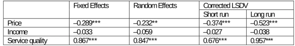
elasticities are reported in Table 4.

The reported price elasticity is significant in all models and less than unity in absolute value. The estimates lie between –0.232 and –0.523 in equilibrium or the long run. In all cases, transit demand is inelastic to fare changes. Also, as predicted by Doel van den and Kiviet (1995), the static panel models report lower price elasticity values than the long run estimates using dynamic models, though the difference is not large. The price elasticity values are very much in consonance with the literature reported in section 3.0. The lower long run values compared to the literature could be perhaps explained by the fact that, most demand elasticity estimates in the literature have been obtained using datasets from developed countries, while this study is based in India. The low elasticity values, therefore, may

represent the state of economic development in India vis–à–vis estimates in other studies. The inelastic demand may also arise from the fact that only public transit fares are included in this analysis since estimates for user costs and external costs are not available for this study. As a result, these estimates do not reflect the elasticity of demand with respect to the generalized transportation costs for the public bus users.

The literature reports negative income elasticities and characterizes public transit as an inferior good. Even though the estimates presented about report negative income elasticity, since the coefficients are not significant, public transit cannot be characterized as an inferior good in India. These results are similar to Maunder (1984) where again income effects are reported to be insignificant in India above a minimum threshold of income. Dargay and Hanly (1999) report that the negative income elasticity during the period of analysis in their study of the United Kingdom between 1970 and 1998 coincided with a rapid increase in personal vehicle ownership. This may be the case in this study as well, given the rapid increase in

personal vehicle population in India during the period under consideration and the significant negative coefficient obtained for personal vehicle ownership in most models.

Service quality is an important variable for influencing transit demand. Again, this is as expected since the constraining factor for most infrastructure services in India, including public bus transit, is availability (Lago and Mayworm (1981)). Fouracre and Maunder (1987) also report in their limited analysis of three Indian cities that a higher level of service results in a higher demand for public transit. However, as noted earlier, increasing the share of public transport through a denser network of routes would call for a cost–benefit analysis of using service quality as a policy tool to increase demand for public transport.

7.0 Conclusions

The economic growth that India has witnessed over the last few years has resulted in rapidly rising transport needs. Simultaneously, concerns are being raised about the

sustainability of the transport sector in the country given a significant and rising share in emissions, both global and local. A well–developed transport system has positive implications for access to healthcare, education, and other basic needs. In the case of passenger road transport, meeting mobility requirements efficiently and addressing environmental and developmental concerns requires a greater share of bus transport in aggregate travel demand. Public transport operators and governments, therefore, need to focus much more on factors influencing demand.

There are two key policy implications that arise from the above analysis. First, the role of pricing is limited with public bus transit demand being price inelastic. Second, factors such as demographic changes and social variables have a larger influence on demand. Access to a public bus transport network has a much larger impact on aggregate demand. If the policy objective is to raise public transit ridership to meet environmental or energy goals, service quality is an important factor affecting demand. However, it is noted that service quality also

depends on revenues to finance quality improvements, which in turn would lead to higher costs and hence fares (Cervero (1990)). Therefore, before investing in the creation of a denser public network of routes, a cost–benefit analysis may be required. Moreover, other parameters affecting transit demand, including other measures of service quality such as travel time, safety, security, and comfort may need to be considered.

Annex. Economic impact of decreasing price compared to

increasing density of coverage

From the log linear demand function specified in section 4 and the RE estimation results in Table 3, and using median values to characterize a representative consumer, the demand function can be expressed as the following:





 

o w q s pop work lit

d pop

p pkm e

w q work lit x median x

                 

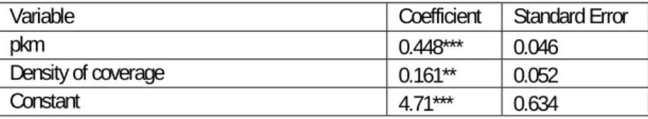
On the cost side, a very small unbalanced panel of 25 public bus companies operating in India between 1990/91 and 2003/04 public bus transit firms is available and a simple log – log Random Effects Cost function has been estimated. In total, 300 observations were available. Output elasticity is 0.448 while the cost elasticity of the density of coverage is 0.161. In addition, this industry is characterized by declining average costs and hence is a natural monopoly.

Table 5 presents the parameter estimates and standard errors of the cost function. Both parameter estimates are statistically significant and carry the expected sign.

The equilibrium price and quantity is then solution of the following system:





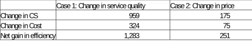
To assess the impact of a change in firm profits and consumer surpluses, simulation results of a service quality increase by 10% are presented in Table 6. The results are presented in terms of equilibrium prices in rupees per passenger kilometers, quantities in terms of

million passenger kilometers, profits of a representative monopoly firm, and consumer surplus of a representative consumer.

As expected, a 10% increase in density of coverage from its mean value results in an increase in consumer surplus (Table 6). In addition, given the results from the cost estimation that this industry is characterized by declining average costs, an increase in density of

coverage leads to a decrease of the average cost and therefore to a fall in loss levels. This counter-intuitive result can be explained by the fact that despite density of coverage (q) having a positive coefficient in the cost function, the increase in equilibrium quantity due to increase in demand from the change in service quality leads to a larger fall in loss levels.

Case 2: Decrease in price

The 10% increase in demand achieved in case 1, can also be achieved by reducing price. Using the price elasticity reported in Table 4, one can then estimate the change in consumer surplus. Similarly, given the estimation results in Table 5, the change in cost levels can be estimated. These are reported in Table 6. As with the earlier case, an increase in output leads to a fall in average costs due.

8.0 References

Abrate, G., M. Piacenza, et al. (2007). The Impact of Integrated Tariff Systems on Public Transport Demand: Evidence from Italy. XIX Riunione scientifica SIEP, Pavia. Appelbaum, E. and J. Berechman (1991). "Demand conditions, regulation, and the

measurement of productivity." Journal of Econometrics 47(2–3): 379–400.

Arellano, M. and S. Bond (1991). "Some Tests of Specification for Panel Data: Monte Carlo Evidence and an Application to Employment Equations." The Review of Economic Studies 58(2): 277-297.

Balcombe, R., R. Mackett, et al. (2004). The demand for public transport: a practical guide. Transportation Research Laboratory Report. London, Transportation Research Laboratory: 246.

Baltagi, B. H. (1986). "Pooling under Misspecification: Some Monte Carlo Evidence on the Kmenta and the Error Components Techniques." Econometric Theory 2(3): 429-440. Baltagi, B. H. (2002). Econometric Analysis of Panel Data. New York, John Wiley.

Beck, N. and J. N. Katz (1995). "What to do (and not to do) with Time-Series Cross-Section Data." The American Political Science Review 89(3): 634-647.

Berechman, J. (1993). Public Transit Economics and Deregulation Policy. Amsterdam, North–Holland.

Blundell, R. and S. Bond (1998). "Initial conditions and moment restrictions in dynamic panel data models." Journal of Econometrics 87(1): 115-143.

Bresson, G., J. Dargay, et al. (2003). "The main determinants of the demand for public transport: a comparative analysis of England and France using shrinkage estimators." Transportation Research Part A: Policy and Practice 37(7): 605–627.

Bun, M. J. G. and F. Windmeijer (2007). The Weak Instrument Problem of the System GMM Estimator in Dynamic Panel Data Models. London, The Institute for Fiscal Studies, Department Of Economics, University College London: 32.

Cameron, A. C. and P. K. Trivedi (2005). Microeconometrics: Methods and Applications. New York, Cambridge University Press.

Census of India 2001 (2001). Census of India 2001, Office of the Registrar General India, Government of India.

Cervero, R. (1990). "Transit pricing research: A review and synthesis." Transportation 17(2): 117-139.

CIRT (Various years). State Transport Undertakings: Profile and Performance. Pune, Central Institute of Road Transport.

Clements, K. W. and S. Selvanathan (1994). "Understanding consumption patterns." Empirical Economics 19(1): 69-110.

Dargay, J. and M. Hanly (1999). Bus Fare Elasticities. Report to the UK Department of the Environment, Transport and the Regions. London, ESRC Transport Studies Unit, University College London: 132.

Dargay, J. M. and M. Hanly (2002). "The Demand for Local Bus Services in England." Journal of Transport Economics and Policy 36(1): 73-91.

de Rus, G. (1990). "Public transport demand in Spain." Journal of Transport Economics and Policy 24(2): 189–201.

Deb, K. (2003). "Restructuring Urban Public Transport in India." Journal of Public Transportation 5(3): 85-102.

Doel van den, I. T. and J. F. Kiviet (1995). "Neglected Dynamics in Panel Data Models: Consequences and Detection in Finite Samples." Statistica Neerlandica 49: 343-361. EPWRF (2003). Domestic Product of States of India: 1960-61 to 2000-01. Mumbai,

Economic and Political Weekly Research Foundation.

Fitzroy, F. R. and I. Smith (1993). The Demand for Public Transport: Some Estimates from Zurich. Fife, Centre for Research into Industry, Enterprise, Finance and the Firm. FitzRoy, F. R. and I. Smith (1997). Passenger Rail Transport: Demand and Quality in a

European Panel. Fife, Centre for Research into Industry, Enterprise, Finance and the Firm.

Fouracre, P. R. and D. A. C. Maunder (1987). Travel demand characteristics in three medium-sized Indian cities. Transport and Road Research Laboratory Research Report 121. Crowthorne, Transport and Road Research Laboratory: 22.

Gandhi, P. J. (1999). "Bus Nationalisation in India: Retrospective-cum-Prospective Reflections." Indian Journal of Transport Management: 181-189.

Goodwin, P. B. and H. C. W. L. Williams (1985). "Public transport demand models and elasticity measures: An overview of recent British experience." Transportation Research Part B: Methodological 19(3): 253-259.

Government of India (2005). Economic Survey 2004/2005. New Delhi, Ministry of Finance, Government of India.

Gowda, J. M. (1999). "Implications of Concessional Travel Facility on the Commercial Viability of SRTCs in India." Indian Journal of Transport Management: 149-157. Hanly, M. and J. Dargay. (1999). "Bus Fare Elasticities: A Literature Review. Report to the

UK Department of the Environment, Transport and the Regions." Retrieved 17 July 2006, from www.cts.ucl.ac.uk/tsu/papers/BusElasticitiesLiteratureReview.pdf. Jovicic, G. and C. O. Hansen (2003). "A passenger travel demand model for Copenhagen."

Transportation Research Part A: Policy and Practice 37(4): 333–349.

Judson, R. A. and A. L. Owen (1999). "Estimating dynamic panel data models: a guide for macroeconomists." Economics Letters 65(1): 9-15.

Justus, E. R. (1998). "Operational Efficiency in Public Passenger Road Transport-A Criteria Analysis." Indian Journal of Transport Management: 573-577.

Kemp, M. A. (1973). "Some evidence of transit demand elasticities." Transportation 2(1): 25-52.

Kiviet, J. F. (1995). "On bias, inconsistency, and efficiency of various estimators in dynamic panel data models." Journal of Econometrics 68(1): 53-78.

Kmenta, J. (1978). Some Problems of Inference from Economic Survey Data. Survey

Sampling and Measurement. N. K. Namboodiri. New York, Academic Press: Chapter 8: 107-120.

Lago, A. and P. Mayworm (1981). "Transit service elasticities." Journal of Transport Economics and Policy 15(2): 99-119.

Matas, A. (2004). "Demand and Revenue Implications of an Integrated Public Transport Policy: The Case of Madrid." Transport Reviews 24(2): 195-217.

Matteo, L. D. (1997). "The Determinants of Wealth and Asset Holding in Nineteenth-Century Canada: Evidence from Microdata." The Journal of Economic History 57(4): 907-934. Maunder, D. A. C. (1984). Trip rates and travel patterns in Delhi, India. Transport and Road

Research Laboratory Research Report 1. Crowthorne, Transport and Road Research Laboratory: 24.

Maunder, D. A. C. (1986). Public transport needs of the urban poor in Delhi. CODATU III, Cairo, International Union of Railways.

Mohring, H. (1970). "The Peak Load Problem with Increasing Returns and Pricing Constraints." The American Economic Review 60(4): 693–705.

MTS. (Various Issues). "Motor Transport Statistics." Retrieved 24 August 2005, 2005, from

http://morth.nic.in/mts.htm.

Nickell, S. (1981). "Biases in Dynamic Models with Fixed Effects." Econometrica 49(6): 1417-1426.

Nickell, S. (1981). "Biases in Dynamic Models with Fixed Effects." Econometrica 49: 1417-1426.

Oehlert, G. W. (1992). "A Note on the Delta Method." The American Statistician 46(1): 27-29.

Oum, T. H. (1989). "Alternative Demand Models and their Elasticity Estimates." Journal of Transport Economics and Policy 23(2): 163-187.

Palmner, C., A. Astrop, et al. (1996). The urban travel behaviour and constraints of low income households and females in Pune, India. National Conference on Women's Travel Issues. Baltimore, Maryland. PA 3206/96: 23 - 26.

Planning Commission (2002). 10th Five Year Plan (2002-2007) -Volume II: Sectoral Policies and Programmes. New Delhi, Planning Commission, Government of India.

Ramanathan, R. and J. K. Parikh (1999). "Transport sector in India: an analysis in the context of sustainable development." Transport Policy 6(1): 35-46.

Romilly, P. (2001). "Subsidy and Local Bus Service Deregulation in Britain: A Re-evaluation." Journal of Transport Economics and Policy 35(2): 161-193.

Roodman, D. (2009). "A note on the theme of too many instruments." Oxford Bulletin of Economics and Statistics 71: 135-158.

Sevestre, P. and A. Trognon (1985). "A note on autoregressive error components models." Journal of Econometrics 28(2): 231-245.

Singh, S. K. (2000). "Estimating the Level of Rail- and Road-based Passenger Mobility in India." Indian Journal of Transport Management 24(12): 771-781.

Singh, S. K. (2005). "Review of Urban Transportation in India." Journal of Public Transportation 8(1): 79-96.

STATA (2005). Longitudinal/Panel Data Reference Manual. College Station, Texas, Stata Press.

Stroup, R. H. and M. B. Hargrove (1969). "Earnings and Education in Rural South Vietnam." The Journal of Human Resources 4(2): 215-225.

Thomas, R. L. (1987). Applied Demand Analysis. London and New York, Longman. Wabe, J. S. (1969). "Labour Force Participation Rates in the London Metropolitan Region."

Journal of the Royal Statistical Society. Series A (General) 132(2): 245-264. Winston, C. (1983). "The demand for freight transportation: models and applications."

Table 1. Recent studies estimating demand functions

Paper Variables Functional Form &

Estimation Method Data Price Short run elasticity Income Long run Short run elasticity Service Long run Short run elasticity Long run

Dargay and Hanly

(1999)1

Two models: Bus passenger kilometers per capita and bus trips per capita bus fares, disposable income, car ownership and motoring costs used only in the structural models.

Two types of models: Error Correction Models and Structural Models. Time series of annual observations between 1970 and 1996 for the United Kingdom. From –0.33 to –0.40 for trips. –0.18 to –0.19 for passenger kilometers From –0.62 to –0.95 for trips. –0.43 to –0.92 for passenger kilometers From 0.18 to 0.41 for trips. 0.05 to 0.16 for passenger kilometers From –0.45 to –0.80 for trips. –0.15 to –0.63 for passenger kilometers Romilly

(2001) Bus journeys per capita. Personal disposable income, index of bus fares, index of motoring cost, service frequency measured by vehicle kilometers per person.

Log linear model, estimated as a single equation Auto Regressive Distributed Lag model after corrections for cointigrating relationships. Time series of annual observations between 1953 and 1997 for United Kingdom excluding London. –0.38 –1.03 0.23 0.61 0.11 0.30 Dargay and Hanly (2002)

Bus journeys per capita fare, service level, per capital disposable income, pensioners in population, motoring costs. Partial adjustment Fixed Effects, Random Effects, and Random Coefficient models. Two specifications: log linear, semi log where only fares are in levels and not logs. Panel data between 1987 and 1996 for 46 counties in United Kingdom. From –0.33

Paper Variables Functional Form &

Estimation Method Data Price Short run elasticity Income Long run Short run elasticity Service Long run Short run elasticity Long run

Bresson, Dargay et

al. (2003) 2

Journeys per capita. Mean fare defined as revenue per trip, service measured by vehicle kilometers per capita, disposable income per capita

Two specifications: Semi log with only fares being in levels, and log linear. Estimated as Arellano and Bond fixed coefficients and random coefficient models Panel data of 46 county annual observations in United Kingdom and 62 urban areas in France during 1987 and 1996. –0.53 for England and –0.40 for France –0.73 for England and –0.70 for France –0.48 for England and –0.01 for France –0.66 for England and –0.02 for France –0.71 for England. –0.19 for France –0.97 for England. –0.33 for France 1

Only national level results reported.

2

Table 2. Descriptive Statistics of variables included in the analysis.

Variable Mean Std. Dev. Min Max

Passenger kilometers (105 _km)

Overall 230 194.300 324 248.600 112.570 2 236 124.000

Between 292 371.900

Within 127 504.700

Public transit fare (Rupees# _{per passenger}

kilometer)

Overall 0.089 0.046 0.031 0.384

Between 0.038

Within 0.033

Per capita income

(Rupees per person) Overall _Between 6 073.593 3 430.798 _{3 398.596} 164.383 19 191.890

Within 1 470.881 Density of coverage (105 vehicle km per km2₎ Overall 0.257 0.778 0.0001 4.089 Between 0.868 Within 0.123

Per capita private vehicle ownership (Vehicles per person)

Overall 0.047 0.079 0.005 0.493

Between 0.089

Within 0.017

Population (number) Overall 43 700 000.000 38 300 000.000 719 601.000 166 000 000.000

Between 38 300 000.000

Within 3 029 920.000

Population the labour

force (%) Overall 38.87% _Between 0.048 _0.047 30.87% 49.24%

Within 0.009

Literacy rate (%) Overall 53.55% 0.109 30.57% 80.04%

Between 0.106

Table 3. Regression results

Fixed Effects& _{Random Effects}& _{Arellano–Bond Corrected–LSDV}

Coefficient Standard

Error Coefficient Standard Error Coefficient Standard Error Coefficient Standard Error

Ln(Public transit fare) -0.289*** 0.062 -0.232*** 0.070 -0.428*** 0.057 -0.374*** 0.044 Ln(Per capita income) -0.033 0.040 -0.059 0.046 -0.026 0.025 -0.027 0.024 Ln(Density of coverage) 0.867*** 0.051 0.847*** 0.043 0.717*** 0.134 0.676*** 0.052 Ln(Per capita private vehicle ownership) 0.053 0.076 -0.084 0.078 0.059 0.048 0.037 0.054 Ln(population) -0.856** 0.312 0.927*** 0.074 -0.893** 0.291 -0.500** 0.248 Labour force participation rate 3.615** 1.650 5.557*** 1.476 3.728* 1.830 2.449** 1.085 Literacy rate -2.423** 0.751 -3.736*** 0.676 -2.057*** 0.481 -1.974*** 0.506 Ln(lagged demand) 0.126 0.091 0.294*** 0.056 o  28.440*** 5.149 -2.227 1.425 26.476*** 4.680 F statistic 135.29*** R2 _0.8949 Sargan (p value) 0.21 AR (1) (p value) 0.06 AR (2) (p value) 0.82 &

price and quality variables in these regressions are in the first lags

*Variables significant at 95% confidence level **Variables significant at 99% confidence level ***Variables significant at 99.9% confidence level

Table 4. Price, Income, and Service Quality Elasticity estimates

Fixed Effects Random Effects Corrected LSDV

Short run Long run Price –0.289*** –0.232** –0.374*** –0.523***

Income –0.033 –0.059 –0.027 –0.038

Service quality 0.867*** 0.847*** 0.676*** 0.957*** **Significant at 99% confidence level, *** Significant at 99.9% confidence level

Table 5. Random Effects regression results for a simple cost function

Variable Coefficient Standard Error

pkm 0.448*** 0.046

Density of coverage 0.161** 0.052

Table 6. Impact on firm profit and consumer surplus of an increase in density of coverage and decrease in price to achieve 10% increase in demand.

Case 1: Change in service quality Case 2: Change in price Change in CS 959 175 Change in Cost 324 75 Net gain in efficiency 1,283 251