HAL Id: hal-00295785
https://hal.archives-ouvertes.fr/hal-00295785
Submitted on 16 Nov 2005
HAL is a multi-disciplinary open access
archive for the deposit and dissemination of
sci-entific research documents, whether they are
pub-lished or not. The documents may come from
teaching and research institutions in France or
abroad, or from public or private research centers.
L’archive ouverte pluridisciplinaire HAL, est
destinée au dépôt et à la diffusion de documents
scientifiques de niveau recherche, publiés ou non,
émanant des établissements d’enseignement et de
recherche français ou étrangers, des laboratoires
publics ou privés.
Detection and mapping of polar stratospheric clouds
using limb scattering observations
C. von Savigny, E. P. Ulasi, K.-U. Eichmann, H. Bovensmann, J. P. Burrows
To cite this version:
C. von Savigny, E. P. Ulasi, K.-U. Eichmann, H. Bovensmann, J. P. Burrows. Detection and mapping
of polar stratospheric clouds using limb scattering observations. Atmospheric Chemistry and Physics,
European Geosciences Union, 2005, 5 (11), pp.3071-3079. �hal-00295785�
www.atmos-chem-phys.org/acp/5/3071/ SRef-ID: 1680-7324/acp/2005-5-3071 European Geosciences Union
Chemistry
and Physics
Detection and mapping of polar stratospheric clouds using limb
scattering observations
C. von Savigny, E. P. Ulasi, K.-U. Eichmann, H. Bovensmann, and J. P. Burrows
Institute of Environmental Physics and Remote Sensing (IUP/IFE), University of Bremen, Otto-Hahn-Allee 1, 28 334 Bremen, Germany
Received: 8 April 2005 – Published in Atmos. Chem. Phys. Discuss.: 22 August 2005 Revised: 20 October 2005 – Accepted: 3 November 2005 – Published: 16 November 2005
Abstract. Satellite-based measurements of Visible/NIR limb-scattered solar radiation are well suited for the detec-tion and mapping of polar stratospheric clouds (PSCs). This publication describes a method to detect PCSs from limb scattering observations with the Scanning Imaging Absorp-tion spectroMeter for Atmospheric CartograpHY (SCIA-MACHY) on the European Space Agency’s Envisat space-craft. The method is based on a color-index approach and requires a priori knowledge of the stratospheric background aerosol loading in order to avoid false PSC identifications by stratospheric background aerosol. The method is applied to a sample data set including the 2003 PSC season in the Southern Hemisphere. The PSCs are correlated with coin-cident UKMO model temperature data, and with very few exceptions, the detected PSCs occur at temperatures below 195–198 K. Monthly averaged PSC descent rates are about 1.5 km/month for the −50◦S to −75◦S latitude range and
assume a maximum between August and September with a value of about 2.5 km/month. The main cause of the PSC descent is the slow descent of the lower stratospheric tem-perature minimum.
1 Introduction
Polar stratospheric clouds are of fundamental importance for the formation of the Antarctic ozone hole (Farman et al., 1985) that occurs every year since the early 1980s in South-ern Hemisphere spring. PSCs act as hosts for heterogeneous reactions that transfer chlorine from the reservoir compounds HCl and ClONO2 to Cl2 (Molina et al., 1987). This
pro-cess occurs throughout the polar night. When solar radia-tion reaches the polar lower stratosphere again, Cl2is
pho-tolyzed to active Cl that participates in a series of catalytic
Correspondence to: C. von Savigny
ozone destruction cycles (e.g. Solomon, 1999). The forma-tion of PSCs requires temperatures of less than about 195 K for PSC types Ia (NAT, nitric acid tri-hydrate; crystalline) and Ib (ternary solution of HNO3, H2SO4and H2O; liquid),
and less than about 188 K for PSC type II (H2O ice).
Several different techniques were applied in the past to re-motely sense PSCs. In terms of ground-based methods there are passive spectrometers measuring scattered solar radiation (e.g. Sarkissian et al., 1994; Enell et al., 1999), as well as active LIDAR systems (e.g. Santacesaria et al., 2001). Satel-lite remote sensing techniques to detect PSCs include solar occultation (McCormick et al., 1989; Fromm et al., 1997; Nedoluha et al., 2003), stellar occultation (Vanhellemont et al., 2005), limb scattering (von Savigny et al., 2005a), and IR emission spectroscopy (Spang et al., 2005). Ground-based measurements can provide continuous observations with high temporal resolution, but are limited to a certain location. The spatial coverage of satellite observations de-pends on the method used, but it is a common feature of most satellite methods, that a certain air volume may only be sam-pled once every several days/weeks. The solar occultation measurements generally provide PSC extinction profiles at different wavelengths with high vertical resolution, but can only be performed during orbital sunsets/sunrises. The ge-ographical coverage of solar occultation measurements on a given day is therefore rather limited. Limb scattering obser-vations are limited to the sunlit part of the Earth, whereas stellar occultation and IR emission can in principle by ap-plied both on the sunlit and the dark side of the Earth.
First results on PSC measurements with SCIAMACHY limb scattering observations were already presented in von Savigny et al. (2005a). In this paper we present a more com-prehensive description of the PSC detection method and its performance using the 2003 Southern Hemisphere (SH) PSC season as a sample data set. The paper is structured as fol-lows: in Sect. 2 a brief description of the SCIAMACHY in-strument and the limb scattering geometry is given, followed
3072 C. von Savigny et al.: PSC mapping by limb scattering
2 von Savigny et al.: PSC mapping by limb scattering
are presented in section 4.
2 SCIAMACHY on Envisat
SCIAMACHY, the Scanning Imaging Absorption spectroM-eter for Atmospheric CartograpHY (Bovensmann et al., 1999) is one of ten scientific instruments on board the Euro-pean Space Agency’s (ESA) environmental satellite Envisat. Since its successful launch on March 1, 2002 Envisat orbits the Earth in a polar, sun-synchronous orbit with a 10:00 LST (local solar time) descending node. SCIAMACHY performs spectroscopic observations of scattered, reflected and trans-mitted solar radiation in three different observation geome-tries: Nadir, occultation and limb scattering. In this study only SCIAMACHY limb scattering observations are used. In limb viewing mode, the tangent height range from 0 km to about 100 km is covered in tangent height steps of 3.3 km. At each tangent height step an azimuthal, i.e., horizontal scan is performed corresponding to 960 km at the tangent point. The instantaneous field of view in limb mode is 2.6 km vertically and 110 km horizontally at the tangent point. The spectral range from about 220 nm up to 2380 nm is covered with a wavelength-dependent spectral resolution of 0.2 – 1.5 nm. On the sunlit side of the Earth limb and nadir measurements are performed alternately, leading to about 25 limb measure-ments per orbit. The spatial extent of the limb ground pixels is about 1000 km perpendicular to the flight (and viewing) direction and 500 km parallel to the flight direction.
It has to be mentioned that the SCIAMACHY limb mea-surements during 2003 were affected by pointing errors of up to 3 km caused by inaccurate knowledge of the spacecraft’s attitude and/or position. As a first order pointing correction 1.5 km were subtracted from the tangent heights provided in the Level 1 data files. More information on the pointing problem can be found in von Savigny et al. (2005b).
3 Methodology
PSC particles act as scatterers of solar radiation and there-fore affect the measured limb radiance profiles. Since the PSC particle sizes are not small compared to the wavelength of the solar radiation in the UV/Visible/NIR spectral range, the spectral dependence of their scattering coefficient differs from the Rayleigh λ−4spectral dependence. Hence, the ra-tio (i.e., color rara-tio or color index) of limb radiances at two wavelengths will provide a sensitive indicator for the pres-ence of PSCs. The following aspects have to be considered when selecting a pair of wavelengths suitable for detecting PSCs with a color index approach using limb scattering ob-servations: (a) the wavelengths should not be affected by molecular absorption, or at least as little as possible; (b) the wavelengths must not be shorter than about 400 nm, since the atmosphere becomes optically thick at UV wavelengths for lower stratospheric tangent heights. This is because of the λ−4wavelength dependence of Rayleigh scattering and below 320 nm also because of the absorption in the Huggins
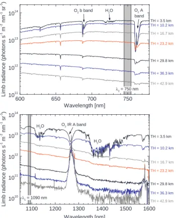
600 650 700 750 1011 1012 1013 1014 O2 b band H2O O2 A band TH = 42.9 km TH = 36.3 km TH = 29.8 km TH = 23.2 km TH = 16.7 km TH = 10.2 km TH = 3.5 km L im b r a d ia n c e ( p h o to n s s -1 m -2 n m -1 s r -1 ) Wavelength [nm] 1100 1200 1300 1400 1500 1600 1010 1011 1012 1013 1014 λ1 = 1090 nm λ2 = 750 nm O2 IR A band H2O H2O TH = 42.9 km TH = 36.3 km TH = 29.8 km TH = 23.2 km TH = 16.7 km TH = 10.2 km TH = 3.5 km L im b r a d ia n c e ( p h o to n s s -1 m -2 n m -1 s r -1 ) Wavelength [nm]
Fig. 1. Limb radiance spectra for SCIAMACHY channels 4 (upper
panel) and 6 (lower panel) for a sample limb observation. Large radiances correspond to low tangent heights and vice versa. The most prominent feature in channel 4 is the O2 A band at 760 nm,
that appears as an absorption feature at low tangent heights and as an emission at higher tangent heights (not shown here). A more detailed description of the spectral features appearing in the spectra can be found in Kaiser et al. (2004a).
and Hartley bands of O3. Please note that 400 nm is only an approximate threshold. The longer the wavelength, the larger is the altitude range where the atmosphere between the tan-gent point and the instrument is optically thin in terms of Rayleigh extinction.
The following wavelengths were chosen: λ1 = 1090 nm (SCIAMACHY channel 6) which is just short of a H2O ab-sorption band ranging from about 1100 nm to 1170 nm; λ2= 750 nm (SCIAMACHY channel 4) between a H2O absorp-tion band centered at 725 nm and the O2A-band (b1Σ+g →
X3Σ−
g) band at around 760 nm. In order to improve the sig-nal to noise ratio we used radiances integrated over ± 5 nm intervals around λ1and λ2. Fig. 1 shows sample limb radi-ance spectra for channels 4 and 6.
In a first step the color index of the limb radiances I(λ,TH) at λ1and λ2is simply determined by
Rc(TH) = I(λ1, TH)
I(λ2, TH) (1)
with TH denoting the tangent height. This approach is
Fig. 1. Limb radiance spectra for SCIAMACHY channels 4 (upper
panel) and 6 (lower panel) for a sample limb observation. Large radiances correspond to low tangent heights and vice versa. The most prominent feature in channel 4 is the O2A band at 760 nm,
that appears as an absorption feature at low tangent heights and as an emission at higher tangent heights (not shown here). A more detailed description of the spectral features appearing in the spectra can be found in Kaiser et al. (2004).
by a summary of the PSC detection technique in Sect. 3. Re-sults on the SH PSC season of 2003, the temporal change of PSC altitudes, and temperatures at PSC altitudes are pre-sented in Sect. 4.
2 SCIAMACHY on Envisat
SCIAMACHY, the Scanning Imaging Absorption spectroM-eter for Atmospheric CartograpHY (Bovensmann et al., 1999) is one of ten scientific instruments on board the Eu-ropean Space Agency’s (ESA) environmental satellite visat. Since its successful launch on 1 March, 2002 En-visat orbits the Earth in a polar, sun-synchronous orbit with a 10:00 LST (local solar time) descending node. SCIA-MACHY performs spectroscopic observations of scattered, reflected and transmitted solar radiation in three different ob-servation geometries: Nadir, occultation and limb scattering. In this study only SCIAMACHY limb scattering observa-tions are used. In limb viewing mode, the tangent height
range from 0 km to about 100 km is covered in tangent height steps of 3.3 km. At each tangent height step an azimuthal, i.e., horizontal scan is performed corresponding to 960 km at the tangent point. The instantaneous field of view in limb mode is about 2.6 km vertically and 110 km horizontally at the tangent point. The spectral range from about 220 nm up to 2380 nm is covered with a wavelength-dependent spectral resolution of 0.2–1.5 nm. On the sunlit side of the Earth limb and nadir measurements are performed alternately, leading to about 25 limb measurements per orbit. The spatial extent of the limb ground pixels is about 1000 km perpendicular to the flight (and viewing) direction and 500 km parallel to the flight direction.
It has to be mentioned that the SCIAMACHY limb mea-surements during 2003 were affected by pointing errors of up to 3 km caused by inaccurate knowledge of the spacecraft’s attitude and/or position. As a first order pointing correction 1.5 km were subtracted from the tangent heights provided in the Level 1 data files. More information on the pointing prob-lem can be found in von Savigny et al. (2005b).
3 Methodology
PSC particles act as scatterers of solar radiation and there-fore affect the measured limb radiance profiles. Since the PSC particle sizes are not small compared to the wavelength of the solar radiation in the UV/Visible/NIR spectral range, the spectral dependence of their scattering coefficient differs from the Rayleigh λ−4spectral dependence. Hence, the ra-tio (i.e., color rara-tio or color index) of limb radiances at two wavelengths will provide a sensitive indicator for the pres-ence of PSCs. The following aspects have to be considered when selecting a pair of wavelengths suitable for detecting PSCs with a color index approach using limb scattering ob-servations: (a) the wavelengths should not be affected by molecular absorption, or at least as little as possible; (b) the wavelengths must not be shorter than about 400 nm, since the atmosphere becomes optically thick at UV wavelengths for lower stratospheric tangent heights. This is because of the λ−4 wavelength dependence of Rayleigh scattering and below 320 nm also because of the absorption in the Huggins and Hartley bands of O3. Please note that 400 nm is only an
approximate threshold. The longer the wavelength, the larger is the altitude range where the atmosphere between the tan-gent point and the instrument is optically thin in terms of Rayleigh extinction.
The following wavelengths were chosen: λ1=1090 nm
(SCIAMACHY channel 6) which is just short of a H2O
absorption band ranging from about 1100 nm to 1170 nm; λ2=750 nm (SCIAMACHY channel 4) between a H2O
ab-sorption band centered at 725 nm and the O2 A-band
(b16g+ → X36g−) band at around 760 nm. In order to im-prove the signal to noise ratio we used radiances integrated
over ±5 nm intervals around λ1and λ2. Figure 1 shows
sam-ple limb radiance spectra for channels 4 and 6.
In a first step the color index of the limb radiances I(λ,TH) at λ1and λ2is simply determined by
Rc(TH) =
I (λ1,TH)
I (λ2,TH)
(1) with TH denoting the tangent height. This approach is sim-ilar to the one used for PSC detection with ground-based UV/Visible spectrometers (e.g. Sarkissian et al., 1994).
In a second step a color index ratio 2(TH) between two adjacent tangent heights is determined from the color index profiles:
2(TH) = Rc(TH)/Rc(TH + 1TH) (2)
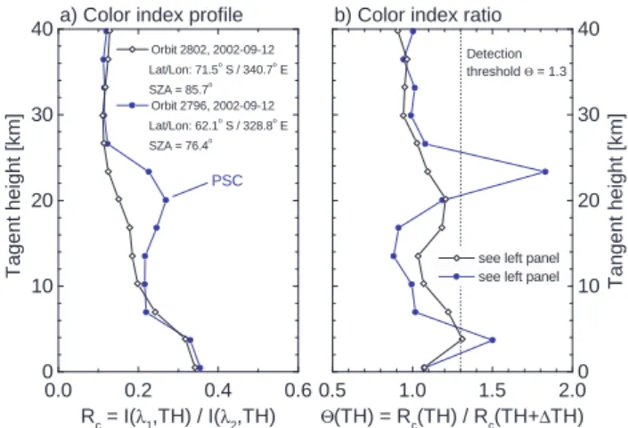
where 1TH=3.3 km is the SCIAMACHY tangent height step. PSCs are detected if the color index ratio 2(TH) ex-ceeds a certain threshold. Figure 2 shows color index pro-files Rc(TH) and color index ratio profiles 2(TH) for two
sample measurements with and without PSCs in the field of view. The use of the color index ratio instead of the color index has proven advantageous, since the color index ratio can be forward-modeled with radiative transfer (RT) calcu-lations even if the measurements are not calibrated. There-fore, radiative transfer calculations can be used as a guide to find an optimum threshold for PSC detection. In order to estimate the range of color index ratios 2(TH) occurring in a PSC-free stratosphere – only due to Rayleigh scattering and stratospheric sulphate aerosol – we performed simula-tions with the RT model LIMBTRAN (Griffioen and Oikari-nen., 2000) for the following scenarios: (a) a pure Rayleigh atmosphere without aerosols, (b) stratospheric background aerosol conditions, (c) moderate volcanic and (d) high vol-canic aerosol conditions and for the solar zenith angle (SZA) range from 30◦ to 90◦, and the solar azimuth angle (SAA) range from 20◦(forward scattering) to 160◦(backward scat-tering). These SZA and SAA ranges include all possi-ble SCIAMACHY limb viewing geometries. The standard MODTRAN aerosol extinction coefficient profiles were used and a Henyey-Greenstein phase function with an asymmetry parameter of g=0.7.
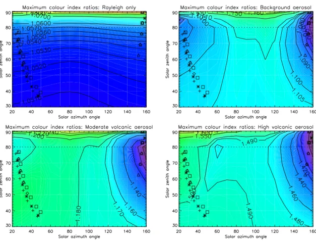
Figure 3 shows contour plots of the modeled maximum color index ratios 2(TH) between 12 and 30 km altitude for the stratospheric aerosol scenarios (a)–(d). The maximum modeled color index ratio 2(TH) for the possible SCIA-MACHY viewing angles are 1.1 for case (a), 1.2 for case (b), 1.3 for case (c), and 1.7 for case (d) for the 15 to 30 km altitude range. Therefore, the threshold for PSC detection re-quires some a priori knowledge of the stratospheric aerosol loading. For the present study – for a low stratospheric aerosols loading – a PSC detection threshold for the color index ratio of 2=1.3 was employed. This implies that opti-cally thin PSCs may not be detected, and the derived statistics is somewhat biased to optically thicker PSCs. Lower color index ratio threshold values (2=1.15, 1.2, 1.25) were also
0 10 20 30 40 0.0 0.2 0.4 0.6
b) Color index ratio a) Color index profile
PSC Orbit 2802, 2002-09-12 Lat/Lon: 71.5o S / 340.7o E SZA = 85.7o Orbit 2796, 2002-09-12 Lat/Lon: 62.1o S / 328.8o E SZA = 76.4o Rc = I(λ1,TH) / I(λ2,TH) T a g e n t h e ig h t [k m ] 0.5 1.0 1.5 2.00 10 20 30 40
see left panel see left panel Ta
n g e n t h e ig h t [k m ] Detection threshold Θ = 1.3 Θ(TH) = Rc(TH) / Rc(TH+∆TH)
Fig. 2. Sample color index profiles (left panel; λ1= 1090 nm, λ2=
750 nm) and color index ratio profiles (right panel) for limb scatter-ing measurements with and without PSCs in the field of view.
similar to the one used for PSC detection with ground-based UV/Visible spectrometers (Sarkissian et al., 1994, e.g.).
In a second step a color index ratio Θ(TH) between two adjacent tangent heights is determined from the color index profiles:
Θ(TH) = Rc(TH)/Rc(TH + ∆TH) (2) where ∆TH = 3.3 km is the SCIAMACHY tangent height step. PSCs are detected if the color index ratio Θ(TH) ex-ceeds a certain threshold. Fig. 2 shows color index pro-files Rc(TH) and color index ratio profiles Θ(TH) for two sample measurements with and without PSCs in the field of view. The use of the color index ratio instead of the color index has proven advantageous, since the color index ratio can be forward-modeled with radiative transfer (RT) calcu-lations even if the measurements are not calibrated. There-fore, radiative transfer calculations can be used as a guide to find an optimum threshold for PSC detection. In order to estimate the range of color index ratios Θ(TH) occurring in a PSC-free stratosphere – only due to Rayleigh scattering and stratospheric sulphate aerosol – we performed simula-tions with the RT model LIMBTRAN (Griffioen and Oikari-nen., 2000) for the following scenarios: (a) a pure Rayleigh atmosphere without aerosols, (b) stratospheric background aerosol conditions, (c) moderate volcanic and (d) high vol-canic aerosol conditions and for the solar zenith angle (SZA) range from 30◦ to 90◦, and the solar azimuth angle (SAA) range from 20◦(forward scattering) to 160◦(backward scat-tering). These SZA and SAA ranges include all possi-ble SCIAMACHY limb viewing geometries. The standard MODTRAN aerosol extinction coefficient profiles were used and a Henyey-Greenstein phase function with an asymmetry parameter of g = 0.7.
Fig. 3 shows contour plots of the modeled maximum color index ratios Θ(TH) between 12 and 30 km altitude for the stratospheric aerosol scenarios (a) - (d). The maximum mod-eled color index ratio Θ(TH) for the possible SCIAMACHY
viewing angles are 1.1 for case (a), 1.2 for case (b), 1.3 for case (c), and 1.7 for case (d) for the 15 to 30 km altitude range. Therefore, the threshold for PSC detection requires some a priori knowledge of the stratospheric aerosol load-ing. For the present study – for a low stratospheric aerosols loading – a PSC detection threshold for the color index ra-tio of Θ = 1.3 was employed. This implies that optically thin PSCs may not be detected, and the derived statistics is somewhat biased to optically thicker PSCs. Lower color in-dex ratio threshold values (Θ = 1.15, 1.2, 1.25) were also tested and led to a significant number of spurious PSC detec-tions. Also shown in Fig. 3 are the viewing angles of SCIA-MACHY limb measurements on different days in Southern Hemisphere Winter/Spring 2003.
Most aspects of the viewing angle dependence of the mod-eled color index ratios in Fig. 3 can be understood qualita-tively.
– For a fixed SZA the Rayleigh scattering phase function is symmetrical with respect to SAA = 90◦, whereas the Mie-phase function favors forward scattering. There-fore, we expect the contour plot for the Rayleigh-only scenario (a) to be more symmetrical with respect to an azimuth angle of 90◦than the scenarios (b) – (d). Fig. 3 shows that this is the case.
– For enhanced stratospheric aerosol loading (scenarios (c) and (d)) the asymmetry of the Mie phase function will become more important, leading to small color in-dex ratios for large solar azimuth angles (backward scat-tering) and large color index ratios for small solar az-imuth angles (forward scattering).
– In all four cases, the maximum color index ratios in-crease for setting sun, i.e., if the SZA approaches 90◦. This is due to the fact, that the Rayleigh extinction coef-ficient and generally also the Mie-extinction coefcoef-ficient at 750 nm is larger than at 1090 nm. Therefore, the at-mosphere is optically thicker at 750 nm than at 1090 nm and the color index ratio increases as the SZA ap-proaches 90◦.
In order to avoid false PSC identifications due to ordi-nary cirrus clouds it was required that the enhancement in the color index ratios has to occur at least 3 km above the climatological tropopause heights taken from Randel et al. (2000).
The advantages of this PSC detection method are (a) that the threshold for PSC detection can be determined indepen-dently with radiative transfer calculations, and (b) that no ad-ditional temperature threshold (e.g., T < 200 K as in Poole and Fritts (1994)) has to be imposed. In terms of (a), the PSC detection methods applied to solar occultation measurements (Poole and Fritts, 1994; Fromm et al., 1997; Hayashida et al., 2000), require empirical aerosol extinction profiles without PSCs to determine the natural variability.
Fig. 2. Sample color index profiles (left panel; λ1=1090 nm,
λ2=750 nm) and color index ratio profiles (right panel) for limb
scattering measurements with and without PSCs in the field of view.
tested and led to a significant number of spurious PSC detec-tions. Also shown in Fig. 3 are the viewing angles of SCIA-MACHY limb measurements on different days in Southern Hemisphere Winter/Spring 2003.
Most aspects of the viewing angle dependence of the mod-eled color index ratios in Fig. 3 can be understood qualita-tively.
– For a fixed SZA the Rayleigh scattering phase function
is symmetrical with respect to SAA=90◦, whereas the
Mie-phase function favors forward scattering. There-fore, we expect the contour plot for the Rayleigh-only scenario (a) to be more symmetrical with respect to an azimuth angle of 90◦than the scenarios (b)–(d). Fig-ure 3 shows that this is the case.
– For enhanced stratospheric aerosol loading (scenarios c
and d) the asymmetry of the Mie phase function will become more important, leading to small color index ratios for large solar azimuth angles (backward scatter-ing) and large color index ratios for small solar azimuth angles (forward scattering).
– In all four cases, the maximum color index ratios
in-crease for setting sun, i.e., if the SZA approaches 90◦. This is due to the fact, that the Rayleigh extinction co-efficient and generally also the Mie-extinction coeffi-cient at 750 nm is larger than at 1090 nm. Therefore, the atmosphere is optically thicker at 750 nm than at 1090 nm and the color index ratio increases as the SZA approaches 90◦.
In order to avoid false PSC identifications due to ordinary cir-rus clouds it was required that the enhancement in the color index ratios has to occur at least 3 km above the climatologi-cal tropopause heights taken from Randel et al. (2000).
30744 C. von Savigny et al.: PSC mapping by limb scatteringvon Savigny et al.: PSC mapping by limb scattering
Fig. 3. Modeled maximum color index gradients Θ(TH) – between 12 and 30 km altitude – for different stratospheric aerosol loadings as a
function of the limb observation angles: solar zenith angle (SZA) and solar azimuth angle (SAA). At SZA = 90◦SAA = 0◦corresponds to forward scattering and SAA = 180◦to backward scattering. For the simulations SZA and SAA were varied in steps of 10◦except for SZA > 80◦, where the SZA was varied in steps of 2◦. The symbols correspond to the viewing angles of the SCIAMACHY measurements on June 15 (plus signs), July 15 (asterisks), August 15 (squares), September 15 (diamonds), and October 15, 2003 (triangles) for latitudes poleward of 50◦(for measurements in the northern/southern hemisphere SAA < 90◦/ > 90◦).
4 Results and Discussion
In order to show that the aerosol signatures identified in the limb radiance measurements are indeed caused by PSCs we investigate in the following sections the geographical distri-bution, the temporal and latitudinal variation of the derived PSC altitudes as well as the temperatures at the altitude of the detected PSCs during the 2003 PSC season in the Southern Hemisphere.
4.1 PSC maps
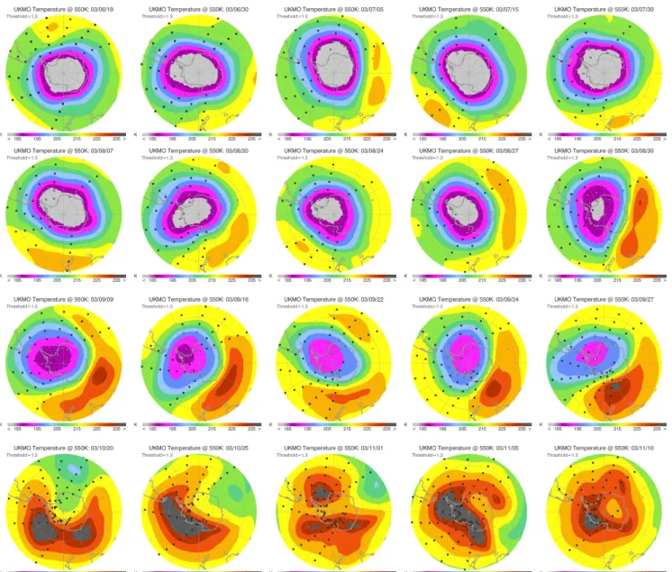
PSC maps for the Southern Hemisphere on selected days be-tween June and November 2003 are shown in Fig. 4. The cir-cles indicate locations of SCIAMACHY limb scattering ob-servations. Black solid circles correspond to measurements without PSC detections and the open circles show detected PSCs. The underlying color contours show the UKMO tem-perature fields for the corresponding days at the 550 K po-tential temperature level. The temperature field is an approx-imate indicator as to where PSCs can be expected. However, 550 K (about 22 km) is generally not identical to the PSC
al-titude – as will be shown in section 4.2 the PSCs descend slowly as the winter progresses. Therefore, apparent out-liers – e.g., the PSCs detected almost above the south pole on September 27, 2003 at temperatures between 200 K and 205 K temperature – are not necessarily PSC occurrences at unrealistically high temperatures. Only up to 10 of the 14 daily orbits are shown for the individual days in Fig. 4. This is because not all the orbits measured are currently available for analysis at IUP/IFE Bremen.
For most days, the detected PSCs occur within the area of sufficiently low temperatures, i.e., roughly below 195 K. The shape of the area covered by PSCs nicely tracks the slowly rotating area of the lower stratospheric temperature minimum. For example, on August 20, 2003 both the vortex and the PSC covered area are slightly elongated and oriented parallel to the 60◦– 240◦meridian. A week later on August 27, 2003 the vortex and the PSC covered area have rotated by about 90◦.
Thus, PSCs are detected in the expected Antarctic regions for sufficiently low temperatures. Note, that due to the used detection method thin PSCs may not be detected. A potential improvement would be the use of color index ratio detection
Fig. 3. Modeled maximum color index gradients 2(TH) – between 12 and 30 km altitude – for different stratospheric aerosol loadings as a function of the limb observation angles: solar zenith angle (SZA) and solar azimuth angle (SAA). At SZA=90◦SAA=0◦corresponds to forward scattering and SAA=180◦to backward scattering. For the simulations SZA and SAA were varied in steps of 10◦except for SZA>80◦, where the SZA was varied in steps of 2◦. The symbols correspond to the viewing angles of the SCIAMACHY measurements on 15 June (plus signs), 15 July (asterisks), 15 August (squares), 15 September (diamonds), and 15 October 2003 (triangles) for latitudes poleward of 50◦(for measurements in the northern/southern hemisphere SAA<90◦/>90◦).
The advantages of this PSC detection method are (a) that the threshold for PSC detection can be determined indepen-dently with radiative transfer calculations, and (b) that no additional temperature threshold (e.g., T <200 K as in Poole and Fritts, 1994) has to be imposed. In terms of (a), the PSC detection methods applied to solar occultation measurements (Poole and Fritts, 1994; Fromm et al., 1997; Hayashida et al., 2000), require empirical aerosol extinction profiles without PSCs to determine the natural variability.
4 Results and discussion
In order to show that the aerosol signatures identified in the limb radiance measurements are indeed caused by PSCs we investigate in the following sections the geographical distri-bution, the temporal and latitudinal variation of the derived PSC altitudes as well as the temperatures at the altitude of the detected PSCs during the 2003 PSC season in the Southern Hemisphere.
4.1 PSC maps
PSC maps for the Southern Hemisphere on selected days be-tween June and November 2003 are shown in Fig. 4. The cir-cles indicate locations of SCIAMACHY limb scattering ob-servations. Black solid circles correspond to measurements without PSC detections and the open circles show detected PSCs. The underlying color contours show the UKMO tem-perature fields for the corresponding days at the 550 K po-tential temperature level. The temperature field is an approx-imate indicator as to where PSCs can be expected. However, 550 K (about 22 km) is generally not identical to the PSC altitude – as will be shown in Sect. 4.2 the PSCs descend slowly as the winter progresses. Therefore, apparent outliers – e.g., the PSCs detected almost above the south pole on 27 September, 2003 at temperatures between 200 K and 205 K temperature – are not necessarily PSC occurrences at unre-alistically high temperatures. Only up to 10 of the 14 daily orbits are shown for the individual days in Fig. 4. This is be-cause not all the orbits measured are currently available for analysis at IUP/IFE Bremen.
Fig. 4. PSC maps for the Southern Hemisphere for selected days during June to November 2003. The circles correspond to the locations
of SCIAMACHY limb scattering measurements. Detected PSCs are indicated by white circles. The underlying color contours represent the UKMO temperatures on the corresponding days at the 550 K (about 22 km altitude) potential temperature level. Note, that this level is not in all cases identical to the PSC altitude. First row: June, July; second row: August; third row: September; last row: October and November 2003.
thresholds that are a function of the SZA. 4.2 Temporal evolution of PSC altitude
By “PSC altitude” we mean the top tangent height for which the color index ratio Θ(TH) exceeds the threshold of Θ = 1.3. Since it contains no information about the vertical extension of the PSC, the PSC altitude is a measure for the PSC top altitude and not for the mean PSC altitude. Note that the actual PSC top altitude will be larger – roughly by about half a tangent height step, i.e., 1.5 to 2 km – than the PSC altitudes
shown here, since we use the TH, where the color index ratio exceeds Θ = 1.3 to determine the PSC altitude.
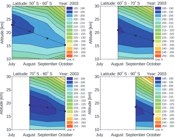
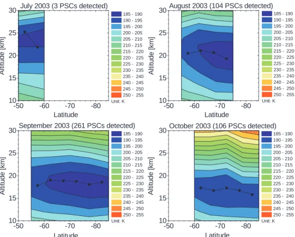
Fig. 5 shows the temporal change of the monthly mean and zonally averaged PSC altitudes for different latitude bands. The latitudinal variation of the monthly mean zonally av-eraged PSC altitudes is shown in Fig. 6 for July to Oc-tober 2003. For the higher latitude ranges SCIAMACHY limb measurements were possible only later in the SH win-ter/spring (see incomplete coverage in Fig. 5), since the high latitude air volumes were not illuminated before.
The color contours show the corresponding mean UKMO
Fig. 4. PSC maps for the Southern Hemisphere for selected days during June to November 2003. The circles correspond to the locations
of SCIAMACHY limb scattering measurements. Detected PSCs are indicated by white circles. The underlying color contours represent the UKMO temperatures on the corresponding days at the 550 K (about 22 km altitude) potential temperature level. Note, that this level is not in all cases identical to the PSC altitude. First row: June, July; second row: August; third row: September; last row: October and November 2003.
For most days, the detected PSCs occur within the area of sufficiently low temperatures, i.e., roughly below 195 K. The shape of the area covered by PSCs nicely tracks the slowly rotating area of the lower stratospheric temperature minimum. For example, on 20 August 2003 both the vortex and the PSC covered area are slightly elongated and oriented parallel to the 60◦–240◦meridian. A week later on 27 Au-gust 2003 the vortex and the PSC covered area have rotated by about 90◦.
Thus, PSCs are detected in the expected Antarctic regions for sufficiently low temperatures. Note, that due to the used
detection method thin PSCs may not be detected. A potential improvement would be the use of color index ratio detection thresholds that are a function of the SZA.
4.2 Temporal evolution of PSC altitude
By “PSC altitude” we mean the top tangent height for which the color index ratio 2(TH) exceeds the threshold of 2=1.3. Since it contains no information about the vertical extension of the PSC, the PSC altitude is a measure for the PSC top altitude and not for the mean PSC altitude. Note that the actual PSC top altitude will be larger – roughly by about half
3076 C. von Savigny et al.: PSC mapping by limb scattering
6
von Savigny et al.: PSC mapping by limb scattering
10 15 20 25 30 185 - 190 190 - 195 195 - 200 200 - 205 205 - 210 210 - 215 215 - 220 220 - 225 225 - 230 230 - 235 235 - 240 240 - 245 245 - 250 250 - 255 Unit: K Latitude: 50o S - 60o S Year: 2003
July August September October
A lt it u d e [ k m ] 10 15 20 25 30 185 - 190 190 - 195 195 - 200 200 - 205 205 - 210 210 - 215 215 - 220 220 - 225 225 - 230 230 - 235 235 - 240 240 - 245 245 - 250 250 - 255 Unit: K Latitude: 60o S - 70o S Year: 2003
July August September October
A lt it u d e [ k m ] 10 15 20 25 30 185 - 190 190 - 195 195 - 200 200 - 205 205 - 210 210 - 215 215 - 220 220 - 225 225 - 230 230 - 235 235 - 240 240 - 245 245 - 250 250 - 255 Unit: K Latitude: 70o S - 80o S Year: 2003
July August September October
A lt it u d e [ k m ] 10 15 20 25 30Latitude: 80 o S - 90o S Year: 2003
July August September October
185 - 190 190 - 195 195 - 200 200 - 205 205 - 210 210 - 215 215 - 220 220 - 225 225 - 230 230 - 235 235 - 240 240 - 245 245 - 250 250 - 255 Unit: K A lt it u d e [ k m ]
Fig. 5. Temporal evolution of mean PSC altitudes for different
lati-tude bands superimposed to the averaged UKMO temperature
pro-files at the locations of the SCIAMACHY limb measurements.
temperature field determined by averaging the UKMO
tem-perature profiles extracted for the date, time and location of
each individual PSC observation. Obviously both the PSC
altitudes and the altitude of the temperature minimum
de-scend slowly with time, and these altitudes are in very good
agreement.
The slow descent of PSCs as the winter progresses has
also been reported in other studies, using ground-based
LI-DAR and solar occultation measurements. Santacesaria et al.
(2001) report on a 9 year (1989 – 1997) PSC climatology
based on LIDAR observations at the French Antarctic base
-50 -60 -70 -80 10 15 20 25 30 185 - 190 190 - 195 195 - 200 200 - 205 205 - 210 210 - 215 215 - 220 220 - 225 225 - 230 230 - 235 235 - 240 240 - 245 245 - 250 250 - 255 Unit: K July 2003 (3 PSCs detected) Latitude A lt it u d e [ k m ] -50 -60 -70 -80 10 15 20 25 30 185 - 190 190 - 195 195 - 200 200 - 205 205 - 210 210 - 215 215 - 220 220 - 225 225 - 230 230 - 235 235 - 240 240 - 245 245 - 250 250 - 255 Unit: K August 2003 (104 PSCs detected) Latitude A lt it u d e [ k m ] -50 -60 -70 -80 10 15 20 25 30 185 - 190 190 - 195 195 - 200 200 - 205 205 - 210 210 - 215 215 - 220 220 - 225 225 - 230 230 - 235 235 - 240 240 - 245 245 - 250 250 - 255 Unit: K September 2003 (261 PSCs detected) Latitude A lt it u d e [ k m ] -50 -60 -70 -80 10 15 20 25 30October 2003 (106 PSCs detected) 185 - 190 190 - 195 195 - 200 200 - 205 205 - 210 210 - 215 215 - 220 220 - 225 225 - 230 230 - 235 235 - 240 240 - 245 245 - 250 250 - 255 Unit: K Latitude A lt it u d e [ k m ]
Fig. 6. Latitude dependence of mean PSC altitudes for different
months of the year 2003 superimposed to the averaged UKMO
tem-perature profiles at the locations of the SCIAMACHY limb
mea-surements.
in Dumont d’Urville (66.40
◦
S, 140.01
◦
E). The authors
dis-cuss three possible reasons for the PSC descent. First, the
sedimentation of the PSC particles, which – stated by
San-tacesaria et al. (2001) – can be excluded as an explanation
for the apparent descent, since the sedimentation speeds are
too large. PSC type II particles can indeed reach
sedimen-tation velocities on the order of 1 km / day, which is
sig-nificantly larger than the observed PSC descent rates.
How-ever, the sedimentation velocities of type I PSCs are smaller
– as small as 10 m / day – and may be consistent with an
apparent PSC descent rate of 1.5 – 2.5 km / month.
Sec-ondly, the slow diabatic descent of the HNO
3
and H
2
O
dis-tributions. This process leads to descent rates of less than
0.5 km / month, and is therefore not strong enough to solely
cause the observed descent. Thirdly, the descent of the lower
stratospheric temperature minimum. Our PSC observations
together with the UKMO temperature data strongly indicate
that the stratospheric temperature is the main driver for the
PSC descent.
The PSC descent rates derived from our measurements for
2003 are: 2.5 km / month for the 50
◦
S – 60
◦
S latitude
band, 2.0 km / month for the 60
◦
S – 70
◦
S latitude band,
and 1.2 km / month for latitudes between 70
◦
S and 80
◦
S.
Interestingly, the descent rates increase with decreasing
lati-tude. These values are in very good agreement with the
LI-DAR measurements by Santacesaria et al. (2001) at Dumont
d’Urville yielding about 2.0 – 2.5 km / month. It is important
to note, that we use a derived PSC altitude that is more
rep-resentative for the PSC top altitude, whereas (Santacesaria
et al., 2001) show mid-cloud altitudes. However,
Santace-saria et al. (2001) mention explicitly that the descent rates
derived from the cloud tops do not differ significantly from
the mid-cloud altitude descent rates. A PSC descent with
rates of about 2.0 km / month was also observed in POAM II
solar occultation measurements (Fromm et al., 1997) during
Southern Hemisphere springs of 1994 – 1996. The latitudes
of the occultation observations varied slowly between about
65
◦
S and 88
◦
S from June to October. Vanhellemont et al.
(2005) recently presented measurements of the extinction by
stratospheric background aerosols and PSCs with GOMOS
(Global Ozone Monitoring by Occultation of Stars), another
remote sensing instrument on Envisat. Although no PSC
de-scent rates were derived, the observed PSC dede-scent is in good
agreement with the results presented here.
From the very good agreement of descent rates of the
temperature minimum and the PSC descent rates derived in
this study it appears that the temporal variation of the lower
stratospheric temperature structure is the main driver of the
PSC descent.
4.3
Distribution of temperature at PSC altitudes
Generally, type I PSCs are assumed to form at temperatures
below about 195 K, and type II PSCs at temperatures below
188 – 190 K. It is important to realize that these threshold
temperatures are not constant, but depend on the amount of
the molecular species the PSC are composed of, i.e., HNO
3
,
Fig. 5. Temporal evolution of mean PSC altitudes for different latitude bands superimposed to the averaged UKMO temperature profiles at
the locations of the SCIAMACHY limb measurements.
a tangent height step, i.e., 1.5 to 2 km – than the PSC altitudes shown here, since we use the TH, where the color index ratio exceeds 2=1.3 to determine the PSC altitude.
Figure 5 shows the temporal change of the monthly mean and zonally averaged PSC altitudes for different latitude bands. The latitudinal variation of the monthly mean zon-ally averaged PSC altitudes is shown in Fig. 6 for July to October 2003. For the higher latitude ranges SCIAMACHY limb measurements were possible only later in the SH win-ter/spring (see incomplete coverage in Fig. 5), since the high latitude air volumes were not illuminated before.
The color contours show the corresponding mean UKMO temperature field determined by averaging the UKMO tem-perature profiles extracted for the date, time and location of each individual PSC observation. Obviously both the PSC altitudes and the altitude of the temperature minimum de-scend slowly with time, and these altitudes are in very good agreement.
The slow descent of PSCs as the winter progresses has also been reported in other studies, using ground-based LI-DAR and solar occultation measurements. Santacesaria et al. (2001) report on a 9 year (1989–1997) PSC climatology based on LIDAR observations at the French Antarctic base in Dumont d’Urville (66.40◦S, 140.01◦E). The authors
dis-cuss three possible reasons for the PSC descent. First, the sedimentation of the PSC particles, which – stated by San-tacesaria et al. (2001) – can be excluded as an explanation for the apparent descent, since the sedimentation speeds are too large. PSC type II particles can indeed reach sedimen-tation velocities on the order of 1 km/day, which is signifi-cantly larger than the observed PSC descent rates. However, the sedimentation velocities of type I PSCs are smaller – as small as 10 m/day – and may be consistent with an apparent PSC descent rate of 1.5–2.5 km/month. Secondly, the slow diabatic descent of the HNO3 and H2O distributions. This
process leads to descent rates of less than 0.5 km/month, and is therefore not strong enough to solely cause the observed descent. Thirdly, the descent of the lower stratospheric tem-perature minimum. Our PSC observations together with the UKMO temperature data strongly indicate that the strato-spheric temperature is the main driver for the PSC descent.
The PSC descent rates derived from our measurements for 2003 are: 2.5 km/month for the 50◦S–60◦S latitude band, 2.0 km/month for the 60◦S–70◦S latitude band, and 1.2 km/month for latitudes between 70◦S and 80◦S. Inter-estingly, the descent rates increase with decreasing latitude. These values are in very good agreement with the LIDAR measurements by Santacesaria et al. (2001) at Dumont
C. von Savigny et al.: PSC mapping by limb scattering 3077 10 15 20 25 30 185 - 190 190 - 195 195 - 200 200 - 205 205 - 210 210 - 215 215 - 220 220 - 225 225 - 230 230 - 235 235 - 240 240 - 245 245 - 250 250 - 255 Unit: K Latitude: 50o S - 60o S Year: 2003
July August September October
A lt it u d e [ k m ] 10 15 20 25 30 185 - 190 190 - 195 195 - 200 200 - 205 205 - 210 210 - 215 215 - 220 220 - 225 225 - 230 230 - 235 235 - 240 240 - 245 245 - 250 250 - 255 Unit: K Latitude: 60o S - 70o S Year: 2003
July August September October
A lt it u d e [ k m ] 10 15 20 25 30 185 - 190 190 - 195 195 - 200 200 - 205 205 - 210 210 - 215 215 - 220 220 - 225 225 - 230 230 - 235 235 - 240 240 - 245 245 - 250 250 - 255 Unit: K Latitude: 70o S - 80o S Year: 2003
July August September October
A lt it u d e [ k m ] 10 15 20 25 30 Latitude: 80 o S - 90o S Year: 2003
July August September October
185 - 190 190 - 195 195 - 200 200 - 205 205 - 210 210 - 215 215 - 220 220 - 225 225 - 230 230 - 235 235 - 240 240 - 245 245 - 250 250 - 255 Unit: K A lt it u d e [ k m ]
Fig. 5. Temporal evolution of mean PSC altitudes for different
lati-tude bands superimposed to the averaged UKMO temperature
pro-files at the locations of the SCIAMACHY limb measurements.
temperature field determined by averaging the UKMO
tem-perature profiles extracted for the date, time and location of
each individual PSC observation. Obviously both the PSC
altitudes and the altitude of the temperature minimum
de-scend slowly with time, and these altitudes are in very good
agreement.
The slow descent of PSCs as the winter progresses has
also been reported in other studies, using ground-based
LI-DAR and solar occultation measurements. Santacesaria et al.
(2001) report on a 9 year (1989 – 1997) PSC climatology
based on LIDAR observations at the French Antarctic base
-50 -60 -70 -80 10 15 20 25 30 185 - 190 190 - 195 195 - 200 200 - 205 205 - 210 210 - 215 215 - 220 220 - 225 225 - 230 230 - 235 235 - 240 240 - 245 245 - 250 250 - 255 Unit: K July 2003 (3 PSCs detected) Latitude A lt it u d e [ k m ] -50 -60 -70 -80 10 15 20 25 30 185 - 190 190 - 195 195 - 200 200 - 205 205 - 210 210 - 215 215 - 220 220 - 225 225 - 230 230 - 235 235 - 240 240 - 245 245 - 250 250 - 255 Unit: K August 2003 (104 PSCs detected) Latitude A lt it u d e [ k m ] -50 -60 -70 -80 10 15 20 25 30 185 - 190 190 - 195 195 - 200 200 - 205 205 - 210 210 - 215 215 - 220 220 - 225 225 - 230 230 - 235 235 - 240 240 - 245 245 - 250 250 - 255 Unit: K September 2003 (261 PSCs detected) Latitude A lt it u d e [ k m ] -50 -60 -70 -80 10 15 20 25 30 October 2003 (106 PSCs detected) 185 - 190 190 - 195 195 - 200 200 - 205 205 - 210 210 - 215 215 - 220 220 - 225 225 - 230 230 - 235 235 - 240 240 - 245 245 - 250 250 - 255 Unit: K Latitude A lt it u d e [ k m ]
Fig. 6. Latitude dependence of mean PSC altitudes for different
months of the year 2003 superimposed to the averaged UKMO
tem-perature profiles at the locations of the SCIAMACHY limb
mea-surements.
in Dumont d’Urville (66.40
◦
S, 140.01
◦
E). The authors
dis-cuss three possible reasons for the PSC descent. First, the
sedimentation of the PSC particles, which – stated by
San-tacesaria et al. (2001) – can be excluded as an explanation
for the apparent descent, since the sedimentation speeds are
too large. PSC type II particles can indeed reach
sedimen-tation velocities on the order of 1 km / day, which is
sig-nificantly larger than the observed PSC descent rates.
How-ever, the sedimentation velocities of type I PSCs are smaller
– as small as 10 m / day – and may be consistent with an
apparent PSC descent rate of 1.5 – 2.5 km / month.
Sec-ondly, the slow diabatic descent of the HNO
3
and H
2
O
dis-tributions. This process leads to descent rates of less than
0.5 km / month, and is therefore not strong enough to solely
cause the observed descent. Thirdly, the descent of the lower
stratospheric temperature minimum. Our PSC observations
together with the UKMO temperature data strongly indicate
that the stratospheric temperature is the main driver for the
PSC descent.
The PSC descent rates derived from our measurements for
2003 are: 2.5 km / month for the 50
◦
S – 60
◦
S latitude
band, 2.0 km / month for the 60
◦
S – 70
◦
S latitude band,
and 1.2 km / month for latitudes between 70
◦
S and 80
◦
S.
Interestingly, the descent rates increase with decreasing
lati-tude. These values are in very good agreement with the
LI-DAR measurements by Santacesaria et al. (2001) at Dumont
d’Urville yielding about 2.0 – 2.5 km / month. It is important
to note, that we use a derived PSC altitude that is more
rep-resentative for the PSC top altitude, whereas (Santacesaria
et al., 2001) show mid-cloud altitudes. However,
Santace-saria et al. (2001) mention explicitly that the descent rates
derived from the cloud tops do not differ significantly from
the mid-cloud altitude descent rates. A PSC descent with
rates of about 2.0 km / month was also observed in POAM II
solar occultation measurements (Fromm et al., 1997) during
Southern Hemisphere springs of 1994 – 1996. The latitudes
of the occultation observations varied slowly between about
65
◦
S and 88
◦
S from June to October. Vanhellemont et al.
(2005) recently presented measurements of the extinction by
stratospheric background aerosols and PSCs with GOMOS
(Global Ozone Monitoring by Occultation of Stars), another
remote sensing instrument on Envisat. Although no PSC
de-scent rates were derived, the observed PSC dede-scent is in good
agreement with the results presented here.
From the very good agreement of descent rates of the
temperature minimum and the PSC descent rates derived in
this study it appears that the temporal variation of the lower
stratospheric temperature structure is the main driver of the
PSC descent.
4.3
Distribution of temperature at PSC altitudes
Generally, type I PSCs are assumed to form at temperatures
below about 195 K, and type II PSCs at temperatures below
188 – 190 K. It is important to realize that these threshold
temperatures are not constant, but depend on the amount of
the molecular species the PSC are composed of, i.e., HNO
3
,
Fig. 6. Latitude dependence of mean PSC altitudes for different months of the year 2003 superimposed to the averaged UKMO temperature
profiles at the locations of the SCIAMACHY limb measurements.
d’Urville yielding about 2.0–2.5 km/month. It is important to note, that we use a derived PSC altitude that is more rep-resentative for the PSC top altitude, whereas Santacesaria et al. (2001) show mid-cloud altitudes. However, Santace-saria et al. (2001) mention explicitly that the descent rates derived from the cloud tops do not differ significantly from the mid-cloud altitude descent rates. A PSC descent with rates of about 2.0 km/month was also observed in POAM II solar occultation measurements (Fromm et al., 1997) during Southern Hemisphere springs of 1994–1996. The latitudes of the occultation observations varied slowly between about 65◦S and 88◦S from June to October. Vanhellemont et al.
(2005) recently presented measurements of the extinction by stratospheric background aerosols and PSCs with GOMOS (Global Ozone Monitoring by Occultation of Stars), another remote sensing instrument on Envisat. Although no PSC de-scent rates were derived, the observed PSC dede-scent is in good agreement with the results presented here.
From the very good agreement of descent rates of the temperature minimum and the PSC descent rates derived in this study it appears that the temporal variation of the lower stratospheric temperature structure is the main driver of the PSC descent.
4.3 Distribution of temperature at PSC altitudes
Generally, type I PSCs are assumed to form at temperatures below about 195 K, and type II PSCs at temperatures be-low 188–190 K. It is important to realize that these threshold temperatures are not constant, but depend on the amount of the molecular species the PSC are composed of, i.e., HNO3,
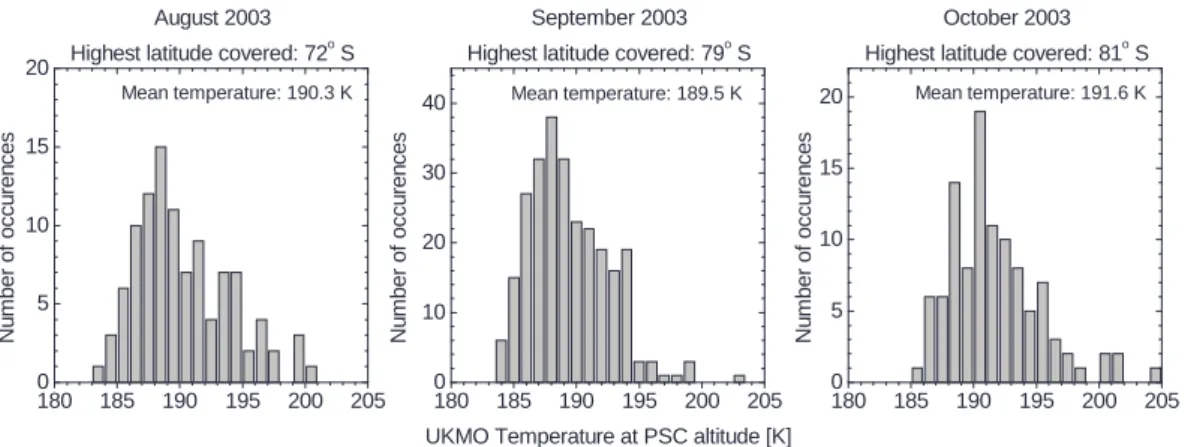
H2SO4and H2O. For all PSCs detected in 2003 the
temper-ature at the PSC altitudes and their locations were extracted from the UKMO temperature fields and are presented as his-tograms for different months in Fig. 7. July 2003 is not shown here, since only 3 PSCs were detected in this month. This low number is due to the fact that the SH polar cap was not illuminated and therefore SCIAMACHY limb scattering measurements were not possible. The average temperatures at the PSC altitudes are around 190 K in August, September, and October 2003, and assume a minimum value of 189.5 K in September. In November no PSCs were detected in agree-ment with temperatures of generally more than 215 K at the 550 K potential temperature level (see Fig. 4). The derived temperatures of around 190 K, at which PSCs are most likely to occur are in very good agreement with previous studies. Santacesaria et al. (2001) report the highest PSC occurrence frequency at a temperature of 189 K. Poole and Fritts (1994)
3078von Savigny et al.: PSC mapping by limb scattering C. von Savigny et al.: PSC mapping by limb scattering7 180 185 190 195 200 205 0 5 10 15 20 Mean temperature: 190.3 K August 2003 Highest latitude covered: 72o S
N u m b e r o f o c c u re n c e s 180 185 190 195 200 205 0 10 20 30 40 Mean temperature: 189.5 K September 2003 Highest latitude covered: 79o S
UKMO Temperature at PSC altitude [K]
N u m b e r o f o c c u re n c e s 180 185 190 195 200 205 0 5 10 15 20 October 2003 Highest latitude covered: 81o S
N u m b e r o f o c c u re n c e s Mean temperature: 191.6 K
Fig. 7. Distribution of the (UKMO) temperatures at the derived PSC locations and altitudes for August September and October 2003. The
mean temperatures at PSC altitude is around 190 K for all three months, and the majority of the detected PSCs occurs at temperatures below 195 K.
H2SO4and H2O. For all PSCs detected in 2003 the
temper-ature at the PSC altitudes and their locations were extracted from the UKMO temperature fields and are presented as his-tograms for different months in Fig. 7. July 2003 is not shown here, since only 3 PSCs were detected in this month. This low number is due to the fact that the SH polar cap was not illuminated and therefore SCIAMACHY limb scattering measurements were not possible. The average temperatures at the PSC altitudes are around 190 K in August, September, and October 2003, and assume a minimum value of 189.5 K in September. In November no PSCs were detected in agree-ment with temperatures of generally more than 215 K at the 550 K potential temperature level (see Fig. 4). The derived temperatures of around 190 K, at which PSCs are most likely to occur are in very good agreement with previous studies. Santacesaria et al. (2001) report the highest PSC occurrence frequency at a temperature of 189 K. Poole and Fritts (1994) find the highest PSC occurrence frequency at 190 K using a 12 years of SAGE II PSC observations. Note, that the low PSC occurrence numbers below temperatures of about 185 K are not due to PSCs not forming at these temperatures, but because only few SCIAMACHY limb scattering obser-vations at locations with lower temperatures are made. The limb scattering observations are limited to the sunlit part of the atmosphere, and therefore the highest southern latitudes with extremely low temperatures during polar night cannot be observed.
The majority of the detected PSCs occurred at tempera-tures of less than 195 K, in good agreement with the expec-tation. There were a few detections at higher temperatures, that may be a consequence of different reasons: (a) due to re-maining errors in the SCIAMACHY limb pointing, the PSCs actually occurred at slightly different altitudes, and therefore different temperatures; (b) larger abundances of the molecu-lar species the PSCs consist of, so that the existence of par-ticles can be maintained at higher temperatures; (c) possibly
small errors in the UKMO temperatures (Pullen and Jones, 1997). In total there were only 7 PSCs detected at apparent temperatures above 200 K. None of them occurred at tem-peratures higher than 205 K.
5 Discussion and Conclusions
In this manuscript we have investigated the detection of PSCs and for the first time the temporal variation of PSC altitudes using limb scattering measurements. This has been achieved with a limited number of wavelengths. As the in-flight cali-bration of SCIAMACHY is improved, we anticipate the ex-tension of the wavelength range to be used to study strato-spheric aerosol, PSCs, and cirrus clouds. PSC type II and cirrus clouds consist of ice particles. In this respect a phase index approach has already been demonstrated to allow the distinction of tropospheric liquid water and ice clouds us-ing Nadir measurements at wavelengths around 1.6 micron. There are several other regions where liquid water and ice absorb in the 0.7 – 2.4 micron region. These absorption sig-natures may be employed for the detection of type II PSCs. This, as well as the use of SCIAMACHY polarization mea-surements, is presently under investigation. Another impor-tant question is whether the SCIAMACHY limb scattering observations with their wide spectral range allow the dis-tinction between type Ia and type Ib PSCs. The principal constituents, i.e., HNO3and H2SO4have no usable
absorp-tion/emission features in the SCIAMACHY spectral range. However, the derivation of PSC particle radii – which is eas-ily possible with noctilucent clouds (NLCs) in the UV spec-tral range (von Savigny et al., 2004), where the strong ab-sorption of solar radiation in the Hartley and Huggins bands of O3lead to negligibly small multiple scattering and surface
reflection contributions – in combination with the measure-ments of the degree of linear polarization may allow to
dis-Fig. 7. Distribution of the (UKMO) temperatures at the derived PSC locations and altitudes for August, September and October 2003. The
mean temperatures at PSC altitude is around 190 K for all three months, and the majority of the detected PSCs occurs at temperatures below 195 K.
find the highest PSC occurrence frequency at 190 K using a 12 years of SAGE II PSC observations. Note, that the low PSC occurrence numbers below temperatures of about 185 K are not due to PSCs not forming at these temperatures, but because only few SCIAMACHY limb scattering obser-vations at locations with lower temperatures are made. The limb scattering observations are limited to the sunlit part of the atmosphere, and therefore the highest southern latitudes with extremely low temperatures during polar night cannot be observed.
The majority of the detected PSCs occurred at tempera-tures of less than 195 K, in good agreement with the expec-tation. There were a few detections at higher temperatures, that may be a consequence of different reasons: (a) due to re-maining errors in the SCIAMACHY limb pointing, the PSCs actually occurred at slightly different altitudes, and therefore different temperatures; (b) larger abundances of the molecu-lar species the PSCs consist of, so that the existence of par-ticles can be maintained at higher temperatures; (c) possibly small errors in the UKMO temperatures (Pullen and Jones, 1997). In total there were only 7 PSCs detected at apparent temperatures above 200 K. None of them occurred at temper-atures higher than 205 K.
5 Discussion and conclusions
In this manuscript we have investigated the detection of PSCs and for the first time the temporal variation of PSC altitudes using limb scattering measurements. This has been achieved with a limited number of wavelengths. As the in-flight cali-bration of SCIAMACHY is improved, we anticipate the ex-tension of the wavelength range to be used to study strato-spheric aerosol, PSCs, and cirrus clouds. PSC type II and cirrus clouds consist of ice particles. In this respect a phase index approach has already been demonstrated to allow the distinction of tropospheric liquid water and ice clouds
us-ing Nadir measurements at wavelengths around 1.6 micron (Kokhanovsky et al., 2005). There are several other regions where liquid water and ice absorb in the 0.7–2.4 micron region. These absorption signatures may be employed for the detection of type II PSCs. This, as well as the use of SCIAMACHY polarization measurements, is presently un-der investigation. Another important question is whether the SCIAMACHY limb scattering observations with their wide spectral range allow the distinction between type Ia and type Ib PSCs. The principal constituents, i.e., HNO3and H2SO4
have no usable absorption/emission features in the SCIA-MACHY spectral range. However, the derivation of PSC par-ticle radii – which is easily possible with noctilucent clouds (NLCs) in the UV spectral range (von Savigny et al., 2004), where the strong absorption of solar radiation in the Hartley and Huggins bands of O3 lead to negligibly small multiple
scattering and surface reflection contributions – in combina-tion with the measurements of the degree of linear polariza-tion may allow to distinguish between type Ia and Ib. This is also the subject of ongoing investigations.
In summary, a method to detect PSCs from limb scattering observations in the Visible/NIR spectral range was presented. The method is based on a color index approach and has been applied to SCIAMACHY limb scattering measurements dur-ing the 2003 PSC season in the Southern Hemisphere. PSC descent rates of 1.0–2.5 km/month were derived, and descent rates were found to increase with increasing latitude. The good correlation between PSC altitude and the altitude of the lower stratospheric temperature minimum leads to the con-clusion that the temporal change of the stratospheric temper-ature field is the main driver behind the observed descent. Concluding, satellite measurements of limb-scattered solar radiation in the Visible/NIR spectral range are a sensitive technique to detect and map PSCs.
Acknowledgements. We thank the European Space Agency (ESA)
for providing the SCIAMACHY data used in this study, the United Kingdom Meteorological Office (UKMO) for providing the UKMO
model data, and Erik Griffioen for making LIMBTRAN available to us. Furthermore, we are indebted to the entire SCIAMACHY team whose efforts make all scientific data analysis possible. This work was in part funded by the University of Bremen and by the German Ministry of Education and Research BMBF (grant 07UFE12/8) and the German Aerospace Center (grant 50EE0027). Edited by: P. C. Simon
References
Bovensmann, H., Burrows, J. P., Buchwitz, M., Frerick, J., No¨el, S., Rozanov, V. V., Chance, K. V., and Goede, A. P. H.: SCIA-MACHY: Mission objectives and measurement modes, J. Atmos. Sci., 56(2), 127–150, 1999.
Enell, C.-F., Steen, ˚A., Wagner, T., Frieß, U., and Platt, U.: Occur-rence of polar stratospheric clouds at Kiruna, Ann. Geophys., 17, 1457–1462, 1999,
SRef-ID: 1432-0576/ag/1999-17-1457.
Fromm, M. D., Bevilacqua, R. M., Lumpe, J. D., Shettle, E. P., Hornstein, J. S., Massie, S. T., and Fricke, K.-H.: Observations of Antarctic polar stratospheric clouds by POAM II: 1994–1996, J. Geophys. Res., 102, 23 659–23 672, 1997.
Farman, J. C., Gardiner, B. G., and Shanklin, J. D.: Large Losses of Total Ozone in Antarctica Reveal Seasonal ClOx/NOx
Inter-action, Nature, 315, 207–210, 1985.
Griffioen, E. and Oikarinen, L.: LIMBTRAN: A pseudo three-dimensional radiative transfer model for the limb-viewing im-ager OSIRIS on the Odin satellite, J. Geophys. Res., 105, D24, 29 717–29 730, 2000.
Hayashida, S., Saitoh, N., Kagawa, A., Yokota, T., Suzuki, M., Nakajima, H., and Sasano, Y.: Arctic polar stratospheric clouds observed with the Improved Limb Atmospheric Spectrometer during winter 1996/1997, J. Geophys. Res., 105, 24 715–24 730, 2000.
Kaiser, J. W., Eichmann, K.-U., No¨el, S., Wuttke, M. W., Skupin, J., von Savigny, C., Rozanov, A. V., Rozanov, V. V., Bovensmann, H., and Burrows, J. P.: SCIAMACHY limb spectra, Adv. Space Res., 34(4), 715–720, 2004.
Kokhanovsky, A. A., Rozanov, V. V., Burrows, J. P., Eichmann, K.-U., Lotz, W., and Vountas, M.: The SCIAMACHY cloud prod-ucts: algorithms and examples from ENVISAT, Adv. Space Res., in press, 2005.
McCormick, M. P., Trepte, C. R., and Pitts, M. C.: Persistence of Polar Stratospheric Clouds in the Southern Polar Region, J. Geo-phys. Res., 94, 11 241–11 251, 1989.
Molina, M. J., Tso, T. L., Molina, L. T., and Wang, F. C.-Y., Antarc-tic Stratospheric Chemistry of Chlorine Nitrate, Hydrogen Chlo-ride and Ice: Release of Active Chlorine, Science, 238, 1253– 1257, 1987.
Nedoluha, G. E., Bevilaqua, R. M., Fromm, M. D., Hoppel, K. W., and Allen, D. R.: POAM measurements of PSCs and water vapor in the 2002 Antarctic vortex, Geophys. Res. Lett., 30(15), 1796, doi:10.1029/2003GL017577, 2003.
Poole, L. R. and Pitts, M. C.: Polar stratospheric cloud climatology based on stratospheric aerosol measurement II observations from 1978 to 1989, J. Geophys. Res., 99, 13 083–13 089, 1994. Pullen, S. and Jones, R. L.: Accuracy of temperatures from UKMO
analyses of 1994/1995 in the Arctic winter stratosphere, Geo-phys. Res. Lett., 24, 845–848, 1997.
Randel, W. J., Wu, W., and Gaffen, D.: Interannual variability of the tropical tropopause derived from radiosonde data and NCEP reanalyses, J. Geophys. Res., 105, 15 509–15 523, 2000. Santacesaria, V., MacKenzie, A. R., and Stefanutti, L.: A
clima-tological study of polar stratospheric clouds (1989–1997) from LIDAR measurements over Dumont d’Urville (Antarctica), Tel-lus, 53B, 306–321, 2001.
Sarkissian, A., Pommereau, J.-P., and Goutail, F.: PSC and volcanic aerosol observations during EASOE by UV-visible ground-based spectroscopy, Geophys. Res. Lett., 21, 1319–1322, 1994. Solomon, S.: Stratospheric ozone depletion: A review of concepts
and history, Reviews of Geophysics, 37, 275–316, 1999. Spang, R., Remedios, J. J., Kramer, L. J., Poole, L. R., Fromm,
M. D., M¨uller, M., Baumgarten, G., and Konopka, K.: Polar stratospheric cloud observations by MIPAS on Envisat: detec-tion method, validadetec-tion and analysis of the northern hemisphere winter 2002/2003, Atmos. Chem. Phys., 5, 679–692, 2005,
SRef-ID: 1680-7324/acp/2005-5-679.
Vanhellemont, F., Fussen, D., Bingen, C., Kyr¨ol¨a, E., Tamminen, J., Sofiefa, V., Hassinen, S., Verronen, P., Sepp¨al¨a, A., Bertaux, J. L., Hauchecorne, A., Dalaudier, F., Fanton d’Andon, O., Barrot, G., Mangin, A., Theodore, B., Guirlet, M., Renard, J. B., Fraisse, R., Snoeij, P., Koopman, R., and Saavedra, L.: A 2003 strato-spheric aerosol extinction and PSC climatology from GOMOS measurements on Envisat, Atmos. Chem. Phys., 5, 2413–2417, 2005,
SRef-ID: 1680-7324/acp/2005-5-2413.
von Savigny, C., Kokhanovsky, A., Bovensmann, H., Eichmann, K.-U., Kaiser, J. W., No¨el, S., Rozanov, A. V., Skupin, J., and Burrows, J. P.: NLC detection and particle size determination: first results from SCIAMACHY on Envisat, Adv. Space Res., 34(4), 851–856, 2004.
von Savigny, C., Rozanov, A., Bovensmann, H., Eichmann, K.-U., No¨el, S., Rozanov, V. V., Sinnhuber, B.-M., Weber, M., and Bur-rows, J. P.: The ozone hole break-up in September 2002 as seen by SCIAMACHY on Envisat, J. Atmos. Sci., 62(3), 721–734, 2005a.
von Savigny, C., Kaiser, J. W., Bovensmann, H., Burrows, J. P., McDermid, I. S., and Leblanc, T.: Spatial and temporal charac-terization of SCIAMACHY limb pointing errors during the first three years of the mission, Atmos. Chem. Phys., 5, 2593–2602, 2005b,