HAL Id: hal-00295330
https://hal.archives-ouvertes.fr/hal-00295330
Submitted on 22 Sep 2003
HAL is a multi-disciplinary open access
archive for the deposit and dissemination of
sci-entific research documents, whether they are
pub-lished or not. The documents may come from
teaching and research institutions in France or
abroad, or from public or private research centers.
L’archive ouverte pluridisciplinaire HAL, est
destinée au dépôt et à la diffusion de documents
scientifiques de niveau recherche, publiés ou non,
émanant des établissements d’enseignement et de
recherche français ou étrangers, des laboratoires
publics ou privés.
stratospheric temperature variations
W. Steinbrecht, B. Hassler, H. Claude, P. Winkler, R. S. Stolarski
To cite this version:
W. Steinbrecht, B. Hassler, H. Claude, P. Winkler, R. S. Stolarski. Global distribution of total
ozone and lower stratospheric temperature variations. Atmospheric Chemistry and Physics, European
Geosciences Union, 2003, 3 (5), pp.1421-1438. �hal-00295330�
www.atmos-chem-phys.org/acp/3/1421/
Chemistry
and Physics
Global distribution of total ozone and lower stratospheric
temperature variations
W. Steinbrecht1, B. Hassler1, H. Claude1, P. Winkler1, and R. S. Stolarski2
1German Weather Service, Hohenpeissenberg, Germany
2NASA, Goddard Space Flight Center, Greenbelt, Maryland, USA
Received: 23 May 2003 – Published in Atmos. Chem. Phys. Discuss.: 3 July 2003
Revised: 10 September 2003 – Accepted: 15 September 2003 – Published: 22 September 2003
Abstract. This study gives an overview of interannual vari-ations of total ozone and 50 hPa temperature. It is based on newer and longer records from the 1979 to 2001 Total Ozone Monitoring Spectrometer (TOMS) and Solar Backscatter Ul-traviolet (SBUV) instruments, and on US National Center for Environmental Prediction (NCEP) reanalyses. Multiple linear least squares regression is used to attribute variations to various natural and anthropogenic explanatory variables. Usually, maps of total ozone and 50 hPa temperature varia-tions look very similar, reflecting a very close coupling be-tween the two. As a rule of thumb, a 10 Dobson Unit (DU) change in total ozone corresponds to a 1 K change of 50 hPa temperature. Large variations come from the linear trend term, up to −30 DU or −1.5 K/decade, from terms related to polar vortex strength, up to 50 DU or 5 K (typical, minimum to maximum), from tropospheric meteorology, up to 30 DU or 3 K, or from the Quasi-Biennial Oscillation (QBO), up to 25 DU or 2.5 K. The 11-year solar cycle, up to 25 DU or 2.5 K, or El Ni˜no/Southern Oscillation (ENSO), up to 10 DU or 1 K, are contributing smaller variations. Stratospheric aerosol after the 1991 Pinatubo eruption lead to warming up to 3 K at low latitudes and to ozone depletion up to 40 DU at high latitudes. Variations attributed to QBO, polar vortex strength, and to a lesser degree to ENSO, exhibit an inverse correlation between low latitudes and higher latitudes. Vari-ations related to the solar cycle or 400 hPa temperature, how-ever, have the same sign over most of the globe. Variations are usually zonally symmetric at low and mid-latitudes, but asymmetric at high latitudes. There, position and strength of the stratospheric anti-cyclones over the Aleutians and south of Australia appear to vary with the phases of solar cycle, QBO or ENSO.
Correspondence to: W. Steinbrecht
1 Introduction
The discovery of the “ozone-hole” over Antarctica in 1984 has triggered enormous interest in stratospheric ozone, both from the general public and from the scientific community. Continuing improvement of our understanding of the various processes controlling the stratospheric ozone layer has since been documented by a wealth of publications (Solomon, 1999; Staehelin et al., 2001) and by a series of ozone assess-ments (SPARC, 1998; WMO, 2003). Production of harm-ful chlorofluorocarbons was successharm-fully curbed by interna-tional agreements, i.e. the Vienna Convention for the Pro-tection of the Ozone Layer (1985), the Montreal Protocol (1987) and its amendments. A reduction of chlorine load-ing and a recovery of the ozone layer are expected at some time in this century (Engel et al., 1998; WMO, 2003). How-ever, stratospheric chlorine will remain high for the next years. Bromine, which also destroys ozone, is still increas-ing. The ozone layer will remain vulnerable. Many details of the expected ozone recovery are unclear, e.g. possible teractions with climate change, or the consequences of in-creasing bromine (Salby and Callaghan, 2002; Ramaswamy et al., 2001; WMO, 2003). In order to actually “see” a recov-ery, high quality measurements are needed for many years to come. For the early detection of signs of a recovery, or of a possible worsening, a good quantitative understanding is necessary for the various natural processes, which contribute to the variation of ozone levels from year to year.
Many studies have investigated variations of ozone and temperature on interannual time scales. This includes trends (Bojkov et al., 1990; Staehelin et al., 2001; Ramaswamy et al., 2001), as well as variations associated with the QBO (Yang and Tung, 1995; Baldwin et al., 2001), the 11-year so-lar cycle (Zerefos et al., 1997; Hood, 1997; Labitzke and van Loon, 2000; Lee and Smith, 2003), the El Ni˜no/Southern Os-cillation (ENSO) (Shiotani, 1992; Zerefos et al., 1992; Reid, 1994), or meteorological factors (Hood et al., 1999; Appen-zeller et al., 2000; Steinbrecht et al., 2001).
The purpose of this study is to give an updated and more global overview of the most relevant sources of variance. Newer and longer data records are used. Rather than focus on global means or zonal averages, the full geographical dis-tribution is presented. A large fraction of the ozone column resides in the lower stratosphere where ozone and tempera-ture are closely linked (Randel and Cobb, 1994). Therefore, analysis of the ozone column data is complemented by analy-sis of lower stratospheric temperature data, at 50 hPa. Where possible, a simple conceptual view is presented, linking to-tal ozone and lower stratospheric temperature variations to a given influence.
2 Data sources and method
The investigation is based on total column ozone data from the series of Total Ozone Mapping Spectrometers (TOMS) and Solar Backscatter Ultraviolet (SBUV and SBUV/2) in-struments on various satellite platforms. All data are cali-brated to be consistent with the 1996 to 1999 Earth-Probe TOMS instrument. See Stolarski and Hollandsworth (2002) for details. The combined data-set currently provides nearly continuous global coverage from late 1978 to December 2001, on a 5◦latitude, 10◦longitude grid. For each grid cell
and each month of the year climatological mean values were defined by the average value over the entire 1979 to 2001 time period. Monthly mean total ozone anomalies were then calculated for each grid cell by subtracting the climatological mean value for the appropriate month of the year. The result-ing anomaly time series are the basis of our investigation.
The same procedure was applied to lower stratospheric temperature fields at 50 hPa from meteorological reanaly-ses by the US National Center for Environmental Prediction (NCEP, Kistler et al., 2001). The NCEP data were regridded to the same latitude-longitude grid as the TOMS/SBUV data. Here we generally report on NCEP data from the same 1979 to 2001 time period where TOMS/SBUV data are available. However, most of the results for 50 hPa temperature change very little, when NCEP data for the longer 1958 to 2001 time period are analysed.
In order to quantify different contributions to total ozone or 50 hPa temperature variations a multiple regression ap-proach is employed (Steinbrecht et al., 2001). This has be-come standard practice (Bojkov et al., 1990; SPARC, 1998; WMO, 2003), but here more predictors are used, in particular meteorological parameters. Anomaly time series Y of total ozone or 50 hPa temperature are described as a linear combi-nation of predictor time series (=explanatory variables), each of which accounts for a different contribution to total ozone or temperature variations:
Y = cT RT R + cF SF S + cAA + cT (400)T (400) +cQBO(10)QBO(10) + cQBO(30)QBO(30) +cu(60N )u(60N ) + cu(60S)u(60S)
+cEN SOEN SO + residual
(1)
Given time series for the explanatory variables trend T R, solar cycle F S, stratospheric aerosol A, 400 hPa temper-ature anomaly T (400), equatorial wind at 10 and 30 hPa
QBO(10/30), zonal wind anomaly at 60◦North and South,
u(60N/S), and El Ni˜no/Southern Oscillation, ENSO, as well as observed time series of ozone or temperature at each grid cell, Y , the coefficients c...can be determined by linear least
squares regression. Global fields for each coefficient are ob-tained as a result. They describe the geographical distribu-tion of the influence for each explanatory variable. Regres-sion was done separately for seasonal mean anomalies, yield-ing separate sets of coefficients cT R, cF S, cQBO(10),and so
on, for winter (December, January , February = DJF), spring (March, April, May = MAM), summer (June, July, August = JJA), and fall (September, October, November = SON). Thus a seasonal variation is allowed for. From the “full” set of possible explanatory variables, only those contributing sig-nificantly, at the 90% confidence level of partial F-tests, were left in the regression, following the stepwise regression pro-cedure outlined in Draper and Smith (1998).
Obviously Eq. (1) is only a very simple approximation. Non-linear effects, as well as possible couplings between ex-planatory variables, are neglected. Generally, only an “aver-age” contribution from each predictor can be obtained. In some years a much stronger or much weaker actual con-tribution must be expected. Nevertheless, our results in-dicate that even this simple approach can still give quite a useful quantification. A more complete picture can be obtained, e.g. with 3-dimensional, fully coupled chemistry global-circulation model simulations. However, such simu-lations are much more complex and more difficult to inter-pret.
2.1 Explanatory variables
The choice of explanatory variables in Eq. (1) is based on the criteria that all should be relevant for total ozone from past experience, and that the data should be easy to obtain and should be updated regularly. The linear trend T R describes long-term ozone changes related to the more or less linear increase of stratospheric chlorine since the 1970s. Most re-cent data show slowing chlorine increase, or very rere-cently, even the beginnings of a decrease (WMO, 2003). However, for compatibility with many other studies, the linear increase was used as a good enough simple description. Improve-ments would be marginal, if a more detailed curve were used (Steinbrecht et al., 2001). For 50 hPa temperature, the linear trend simply describes long-term changes.
10.7 cm solar radio flux F S is a common proxy for UV irradiance changes related to the 11-year solar cycle (Zerefos et al., 1997). Monthly mean data observed in Ottawa and Penticton, Canada, were obtained from ftp://ftp.ngdc.noaa. gov/STP/SOLAR DATA/SOLAR RADIO/FLUX.
For variations related to the Quasi-Biennial Oscillation (QBO), equatorial zonal winds at 10 and 30 hPa QBO(10) and QBO(30) from FU Berlin are included (B. Naujokat, priv. comm. 2003). Correct phasing of the QBO related signal is allowed for by using winds at two levels, 10 and 30 hPa, which are out of phase by nearly π/2 (see Bojkov and Fioletov, 1995).
Large enhancements of stratospheric aerosol after major volcanic eruptions in the tropics affect ozone and tempera-ture by changing heating rates and atmospheric transports. Ozone is additionally affected by heterogeneous reactions on the much increased aerosol surface area (Solomon, 1999; Robock, 2000). To account for these effects, the time de-pendent stratospheric aerosol optical depth A is included as one explanatory variable. We use zonal mean data compiled by Sato (2003), which allow for latitudinal variation. For the period of interest, the data are largely based on mea-surements by the Stratospheric Aerosol and Gas Experiments (SAGE I and II). Note that using stratospheric aerosol opti-cal depth measured by lidar at a single location (Garmisch-Partenkirchen in Southern Germany) (J¨ager et al., 1995) gives very similar results.
The meteorological situation in the troposphere can have a large influence on ozone column and on lower stratospheric temperature (Steinbrecht et al., 1998; Appenzeller et al., 2000). Therefore temperature anomalies at 400 hPa, T (400), were used as one explanatory variable. Temperature in the free troposphere and lower stratosphere is highly correlated with other meteorological parameters such as tropopause height, geopotential heights, or tropospheric circulation in-dices. The T (400) anomaly field was derived from NCEP reanalyses.
Influences from the El Ni˜no–Southern Oscillation phe-nomenon are accounted for by the ENSO explanatory vari-able, obtained from the US National Oceanic and Atmo-spheric Administration, Climate Prediction Center (NOAA-CPC, http://www.cpc.ncep.noaa.gov/data/indices/).
The strength of the polar winter vortex is another impor-tant explanatory variable. A strong vortex is a prerequisite for the formation of an “ozone hole” (Solomon, 1999). Vor-tex strength is also related to meridional transports in the Brewer-Dobson circulation (Perlwitz and Graf, 1995; Salby and Callaghan, 2002). Zonal wind anomalies at 50 hPa, 60◦
North and 60◦South from NCEP reanalyses, u(60N/S), are
a good measure of vortex strength, and were included as ex-planatory variables. Other possibilities are indices for the large scale stratospheric circulation, such as the Arctic Os-cillation Index (Baldwin and Dunkerton, 1999), or the di-vergence of the Eliassen-Palm flux (Salby and Callaghan, 2002). However, we preferred the zonal-winds, because they are easy to obtain from the NCEP reanalyses and seem to work quite well.
2.2 Technical aspects
Linear least squares regression requires that the explanatory variables are sufficiently independent (uncorrelated). While we found that this is generally fulfilled in our case, there are two important exceptions: 1.) The strength of the polar vor-tex is related to the phase of the QBO and the solar cycle (Holton and Tan, 1980; Labitzke and van Loon, 2000). 2.) Tropospheric temperatures T (400) are highly correlated with El Ni˜no/La Ni˜na over large parts of the globe. When two explanatory variables are highly correlated, the stepwise ap-proach tends to include only the more significant explanatory variable, and leave the less significant explanatory variables out of the regression (Draper and Smith, 1998). This avoids technical problems with highly correlated explanatory vari-ables. For the critical cases, results obtained with the full set of predictors are compared to results with a reduced set of predictors. Generally, interdependencies between the ex-planatory variables are small and hardly influence the results. The residual in Eq. (1) is typically a first-order autocorre-lated noise series (Bojkov et al., 1990; SPARC, 1998). How-ever, since seasonal mean data are used, and since the regres-sion usually describes a very large part of the observed vari-ance, autocorrelation was found to be negligible. One years total ozone or temperature residual has little to do with the residual of the previous year. This simplifies the statistical tests and the stepwise linear regression model. Nevertheless, particularly for the solar cycle, it must be realized that the 23 years of 1979 to 2001 data only cover 3 solar maxima and 2 solar minima. Thus we have less than 23 completely in-dependent samples of the solar cycle effect, but likely more than 3. The statistical significance, i.e. the confidence level, of our results may therefore be overestimated, in particular for the longer time-scales of solar cycle or ENSO. Since for 50 hPa temperature very similar results are obtained when using 42 years of NCEP data (1958 to 2001), there does not seem to be a major problem.
2.3 Data quality
A detailed investigation of the data quality of the TOMS/SBUV or NCEP reanalysis data-sets is clearly be-yond the scope of this paper. However, the following dis-cussion indicates that there are no major inconsistencies in the two data-sets. Our results should, therefore, be represen-tative for the “true” atmosphere.
For total ozone, Fioletov et al. (2002) and Harris et al. (2003) have compared various total ozone time se-ries, from ground-based spectrometers, from an assimilated TOMS/GOME/ground-based data-set at NIWA (Bodeker et al., 2001), and from the TOMS/SBUV merged data-set used in this paper. For zonal means over large latitude bands, e.g. 35◦N to 60◦N, Fioletov et al. (2002) report differences be-tween these data sets that vary over time, but are generally less than 1% (≈2 to 4 DU). Harris et al. (2003) only report on
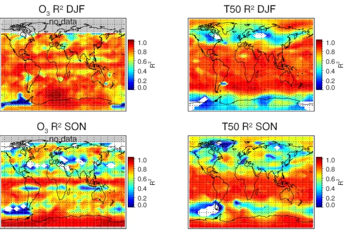
Fig. 1. Global maps of R2from regression of 1978 to 2001 TOMS/SBUV total ozone anomalies on a 5◦latitude by 10◦longitude grid (left panels), or of 1978 to 2001 50 hPa temperature anomalies from NCEP reanalyses (right panels), for winter (DJF, top panels) and fall (SON, bottom panels). No TOMS/SBUV observations are available in polar regions in winter. The corresponding regions are indicated by grey shading.
low-pass filtered data, where most known sources of variabil-ity have been removed, such as solar-cycle, QBO, 500 hPa temperature, etc.. They only consider fluctuations on time-scales longer than the QBO, and do find a smaller longterm trend in the merged TOMS/SBUV data set. Apart from that, they find time varying differences between the data sets that are typically smaller than 1% for selected smaller regions, such as the grid cells used in our analysis. Time varying bias of the merged TOMS/SBUV data-set will certainly affect our results. However, based on Fioletov et al.’s and Harris et al.’s results, it seems that errors should be of the order of 1 to 2%, corresponding to a few Dobson Units. This is comparable to the statistical uncertainty of our results, which is typically larger than 2 to 5 DU. Therefore we think that data consis-tency of the TOMS/SBUV data-set is not a major issue for our analysis.
The NCEP reanalysis data do exhibit quality changes over time which are related mostly to changes in the observing system. The largest known jumps in NCEP reanalyses oc-cur at the introduction of satellite observations in late 1978 (Santer et al., 1999; Trenberth et al., 2001). Since our paper
uses mainly the 1979 to 2001 data, it should not be affected by this major jump. Even when the extended 1958 to 2001 period (major jump in late 1978) is considered, nearly all of our results, except for the linear trend, are very similar to those obtained for the more homogeneous 1979 to 2001 pe-riod. We would expect that possible smaller quality changes after 1979 would result in even less noticable changes. Inde-pendent support for the case of the 11-year solar cycle comes from van Loon and Labitzke (1999), who found very similar results for NCEP reanalysis and Berlin stratospheric analyses for the 1968 to 1996 period, which includes the major jump in NCEP reanalyses.
3 Results
An important measure for the performance of a regression is R2, the ratio of variance described by the regression, i.e. the variance of all terms on the right side of Eq. (1) except for the residual, to observed variance, i.e. to the variance of the left side of Eq. (1). A perfect regression has R2=1 and fully explains the observed variance. Small R2≈0 indicates
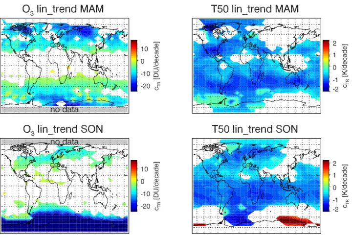
Fig. 2. Left panels: Linear trend, in DU per decade, from multiple regression of 1978 to 2001 TOMS/SBUV total ozone anomalies on a 5◦ latitude by 10◦longitude grid. Right panels: Linear trend, in K per decade, from multiple regression of 1978 to 2001 temperature anomalies at 50 hPa from NCEP reanalyses on a 5◦latitude by 10◦longitude grid. Top panels: Spring (MAM). Bottom panels: Fall (SON). In the white regions the linear trend is not statistically significant at the 90% confidence level. Also note that no TOMS/SBUV observations are available in polar regions in winter. The corresponding regions are indicated by grey shading.
that the regression explains only a small part of the observed variance. This can happen when random noise, e.g. from the measurement itself, accounts for a large fraction of the ob-served variance, or when important explanatory variables are missing. Generally for our study, R2 values are higher in winter and spring, and lower in fall, in the respective hemi-spheres.
As examples for good and relatively poor regression, Fig. 1 shows maps of R2 for Northern Hemisphere winter (DJF) and Northern Hemisphere fall (SON). In DJF, R2for total ozone exceeds 0.7 over most of the observed globe, in-dicating that more than 70 percent of the observed total ozone variance are accounted for by the regression. In some regions the regression works less well, e.g. around 10◦North and 10◦
South, over parts of Russia, or over the Southern Pacific. Re-gression also works less well for SON, where R2falls below 0.4 for a substantial fraction of the Northern Hemisphere, and for some regions in the Southern Hemisphere. An im-portant contributor to the low R2 regions around 10◦ lati-tude, on either side of the equator, is the low natural variance of total ozone there. This makes atmospheric and
observa-tional noise more relevant. To a lesser degree the same ap-plies to the lower R2over the fall hemispheres. The low R2 regions over the Southern Pacific in Southern Hemisphere spring (SON), or over Russia in northern winter (DJF) are more pronounced in the R2 maps for 50 hPa temperature (right panels of Fig. 1).
For 50 hPa temperature, R2is similar for all seasons. R2is high (>0.7) and the regression works well in the tropics and subtropics and in the polar region in winter. However, there are broad bands around 50◦ to 60◦ latitude of each hemi-sphere where R2is low (<0.4). There, the regression does not give a good description. To a lesser degree, these bands also appear in the R2 for total ozone. These bands might come from variations in position and size of jet-streams or polar vortices, not well accounted for by the present set of ex-planatory variables. Additional exex-planatory variables might improve the regression in this latitude band. However, within the scope of the present study, simple additional explanatory variables could not be found. As a consequence, results for the 50◦to 60◦latitude bands have to be interpreted with care.
3.1 Linear trend
Figure 2 shows maps of the linear trend term from Eq. (1) for northern and southern spring. This term describes long-term changes in total ozone, which can largely be attributed to chemical ozone depletion by anthropogenic chlorine and bromine (Staehelin et al., 2001; WMO, 2003). Total ozone has been decreasing over the last 20 years outside of the trop-ics. The decrease is larger at higher latitudes. In both hemi-spheres, the decrease is larger in spring than in fall. By far the largest ozone trends, up to −50 Dobson Units (DU) per decade, are found in the “ozone hole” south of 50◦S in south-ern spring. Fairly high ozone trends, up to −20 DU/decade are also found in northern spring over Siberia. Trends for DJF and JJA (both not shown) are similar to those for MAM and SON, respectively.
Temperature at 50 hPa also shows a significant negative trend over most of the globe, ranging between −0.5 and
−2 K per decade. The trend appears to be larger in the South-ern Hemisphere, and is generally larger in the tropics and subtropics and in the summer and fall hemispheres. Note that the temperature trends exhibit less seasonal variation than the total ozone trends. Smaller negative temperature trends by 0.5 to 1 K, with a similar geographical distribution are found when the regression is applied to NCEP reanalyses for the longer 1958 to 2001 period, not only the 1979 to 2001 period corresponding to the total ozone record.
The ozone trends presented here are fully consistent with other recent investigations, e.g. Fioletov et al. (2002), or WMO (2003). Note, however, that Harris et al. (2003), using a different method, find smaller trends for the same merged TOMS/SBUV data set. Apart from the region south of 60◦S,
where the specific time period considered and questions re-garding consistency of the NCEP reanalysis before 1979 ap-pear to be important, our temperature trends are similar to Ramaswamy et al. (2001).
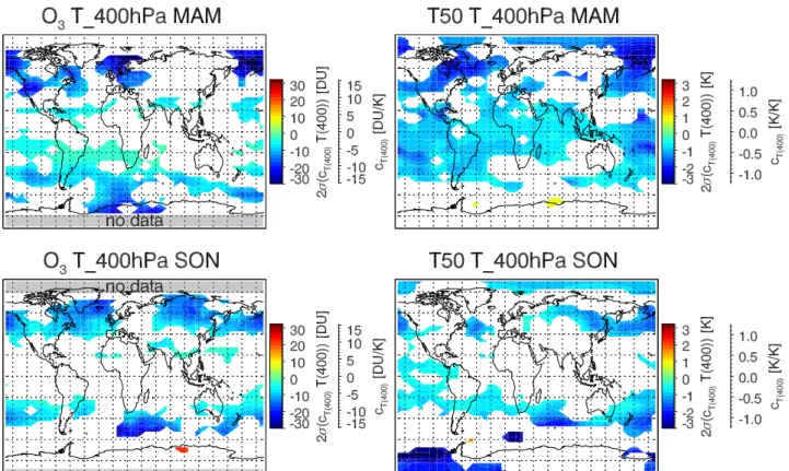
3.2 Variations associated with tropospheric meteorology Temperature anomalies at 400 hPa were included in the re-gression to account for links between tropospheric meteo-rological parameters and total ozone or lower stratospheric temperature (Steinbrecht et al., 1998; Appenzeller et al., 2000; WMO, 2003). Figure 3 shows the size of ozone and 50 hPa temperature fluctuations linked to T (400).
As size of the variation attributed to an explanatory vari-able X, here and in most following plots and discussions, we define 2 standard deviations (2σ ) of the corresponding time series term (cXX) on the right side of Eq. (1). This size
is close to the average minimum-to-maximum variation at-tributed to explanatory variable X. Using 2σ allows an easy comparison of the importance of different explanatory vari-ables. The color plots in Fig. 3, and the following, show this size as a function of latitude and longitude over the globe. Red and yellow colors indicate positive correlation between
ozone, or temperature, and explanatory variable X. Blue col-ors (negative values) indicate inverse correlation. Note that for explanatory variables X that do not vary with latitude or longitude, the second scales on the maps directly give the size of the regression coefficients cX. For explanatory
vari-ables that vary over the map, notably T400and A, the second
scales on the maps can only be approximate.
As Fig. 3 shows, both ozone and 50 hPa temperature fluc-tuations are inversely correlated to tropospheric temperature. The size of the variations generally increases with latitude. In the tropics little or no ozone fluctuations are associated with tropospheric temperature changes. Variations associ-ated with 400 hPa temperature are largest in spring at north-ern high latitudes, where they reach up to 30 DU or 3 K. The overall picture is, however, similar for all seasons and both hemispheres. Total ozone is low and the lower stratosphere is cold when the troposphere is warm, whereas total ozone and lower stratospheric temperature are high when the tropo-sphere is cold.
Part of this behavior can be explained by up- and down-ward air motions in the lower stratosphere, which com-pensate opposite vertical motions in the troposphere (Reed, 1950; Steinbrecht et al., 1998; Labitzke and van Loon, 1999). In a tropospheric high pressure system, sinking air in the tro-posphere leads to adiabatic warming there. The tropopause and air in the lower stratosphere rise. This results in adiabatic cooling in the lower stratosphere and moves ozone poor air up. Total ozone decreases. A tropospheric low pressure sys-tem has vertical motions in the opposite direction, and con-sequently a cold troposphere and a warm, ozone rich lower stratosphere with high total ozone. These vertical motions go hand in hand with horizontal advection, e.g. of ozone poor air from low latitudes, or of ozone rich air from high latitudes in the lower stratosphere (Salby and Callaghan, 1993; Koch et al., 2002). A typical low pressure system advects ozone poor low-latitude air above its tropospheric warm sector, where the tropopause is high, and advects ozone rich high-latitude air above its tropospheric cold sector, where the tropopause is low. Salby and Callaghan (1993) estimate that vertical mo-tions account for about two thirds, and horizontal advection for about one third of the total ozone fluctuations directly associated with meteorology. Note that increased/decreased radiative heating by more/less ozone also tends to give a pos-itive correlation between total ozone and lower stratospheric temperature, especially on longer time-scales (Ramaswamy et al., 2001).
3.3 Influence of the Quasi-Biennial Oscillation
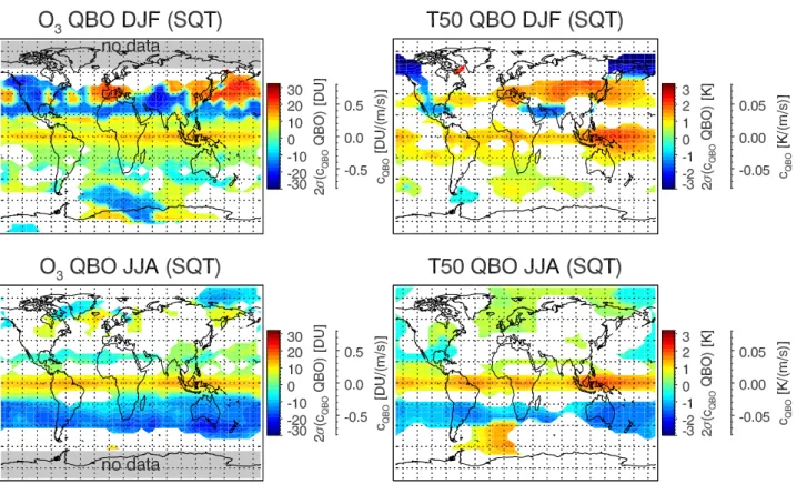
The QBO with its downwards propagating zonal wind anomalies is an intriguing example of wave mean-flow in-teraction in the atmosphere. It has far-ranging effects that can be observed in many atmospheric parameters (Baldwin et al., 2001). Size and geographic distribution of ozone and 50 hPa temperature fluctuations attributed to the QBO by the
Fig. 3. Size of fluctuations attributed to temperature anomalies at 400 hPa. The size is defined as 2 standard deviations, in DU or K, of the term cT (400)T (400) in Eq. (1). The second scales, on the right, give only the approximate size of the regression coefficient cT (400). In this
plot and the following, blue colors (negative values) indicate that ozone or temperature are inversely (negatively) correlated to the explanatory variable, whereas yellow and red colors (positive values) denote positive correlation. In the white regions the explanatory variable is not statistically significant at the 90% confidence level. Also note that no TOMS/SBUV observations are available in polar regions in winter. These regions are indicated by grey shading.
regression in this study are shown in Fig. 4. When equatorial zonal wind is westerly at 30 hPa, total ozone and 50 hPa tem-perature are high in the tropics (yellow and red colors) and are low (green and blue colors) in a subtropical belt from about 20◦ to 40◦ or 50◦. In the winter hemisphere, sub-tropical ozone and temperature anomalies are larger, up to
−25 DU or −2.5 K, than in the summer hemisphere, where they only reach up to −5 DU or −0.5 K. Ozone anomalies in the summer hemisphere also extend to higher latitudes. Size, up to 25 DU or 2.5 K, and annual variation, much larger signal in the winter/spring hemisphere, of QBO related varia-tions found here agree well with previous results summarized by Baldwin et al. (2001).
The tropical and subtropical anomalies can be ex-plained by a QBO-induced residual circulation with de-scending/ascending motion in the tropics and ascend-ing/descending motion in the subtropics (Andrews et al., 1987; Baldwin et al., 2001). This circulation modulates the stronger large-scale Brewer-Dobson circulation, which has an ascending branch in the tropics and descending branches in the extratropics. According to the thermal wind relation, the vertical motions of the QBO residual circulation are
in-duced by the westerly/easterly vertical wind shear associ-ated with the QBO. For the case of westerly wind shear, e.g. when maximum westerly winds are found at or above 30 hPa, the QBO induced circulation is downwards in the tropical lower stratosphere. This slows the general Brewer-Dobson upwelling in the tropics. Less ozone poor air is brought up in the tropical lower stratosphere, thereby increasing trop-ical total ozone. Less upwelling also means less adiabatic cooling and thus a warmer tropical lower stratosphere. It ex-plains the yellow and red band of positive anomalies around the Equator in Fig. 4. In the subtropics the QBO induced circulation is upwards. The general downwelling of ozone rich air in the extratropics from the Brewer-Dobson circula-tion is reduced, thereby decreasing subtropical total ozone. Also, adiabatic heating of the subtropical lower stratosphere is reduced. These regions of decreased downwelling ap-pear as blue bands in Fig. 4. In the winter hemisphere, the subtropical anomaly is enhanced by the strong residual Brewer-Dobson circulation in winter and spring (Baldwin et al., 2001).
While tropical and subtropical variations related to the QBO are zonally symmetric, QBO-related fluctuations at
Fig. 4. Same as Fig. 3, but for fluctuations attributed to the QBO. The scales on the false color bars give 2 standard deviations (2σ ) of the QBO term cQBO(10)QBO(10)+cQBO(30)QBO(30) in Eq. (1). The second scales, on the right, give the approximate size of the QBO
regression coefficientqcQBO(2 10)+cQBO(2 30). Blue colors indicate inverse (negative) correlation with westerly zonal wind at 30 hPa at the Equator, whereas yellow and red colors indicate positive correlation.
higher latitudes in the winter hemispheres, between 40◦and 80◦, are not zonally symmetric: High 50 hPa temperatures, i.e. the red or yellow regions in Fig. 4 occur during QBO-westerlies at 30 hPa from Europe to Northeastern Asia in DJF (and MAM, not shown), north of North-America in SON (not shown), and above the Southern Atlantic Ocean in JJA (and SON as well, not shown). Where TOMS/SBUV data are available, the total ozone maps also indicate variations in these regions. These higher latitude features are out of phase with the subtropical and in phase with the tropical sig-nal. Phase changes in QBO-attributed variations at latitudes around 40◦N or 50◦N have been noted previously (Bojkov
and Fioletov, 1995; Yang and Tung, 1995). Yang and Tung argued that phase changes appear because high-latitude to-tal ozone anomalies in some years have the same sign as anomalies in mid-latitudes. In other years they have the op-posite sign. When projected onto any QBO-predictor, these “missing” beats produce an apparent phase change. Irregular “missing” beats, not accounted for by the regression, would also create a band of low R2, as seen in Fig. 1.
Because of the inclusion of zonal wind anomalies at 60◦, 50 hPa, as one explanatory variable in the regression (see Figs. 10 and 11), QBO modulations related to polar vortex
strength do not appear in Fig. 4. Therefore, Fig. 5 shows re-sults of a regression where trend, solar cycle and QBO were used as the only explanatory variables. For most seasons and latitudes, the QBO signal for this reduced set of explanatory variables is very similar to the QBO signal obtained with the full set of explanatory variables in Fig. 4. The main differ-ence between the two sets of explanatory variables is a dipole between low polar temperatures north of 60◦N and high tem-peratures in a band around 40◦N, that are seen in Fig. 5 for the reduced set of explanatory variables in DJF and SON (not shown), during QBO-westerlies at 30 hPa. Also, high temperatures and high total ozone around 40◦are more
pro-nounced and more zonally symmetric in Fig. 5, compared to Fig. 4. As shown later in Fig. 10, such a see-saw be-tween high and lower latitudes is the signature of polar vor-tex strength. Because the QBO modulates the strength of the polar vortex, parts of the variations related to polar vor-tex strength are taken over by the QBO explanatory variable, when no explanatory variable for polar vortex strength is in-cluded in the regression. This is the case for Fig. 5.
Colder polar temperatures and a stronger polar vortex dur-ing times of QBO-westerlies (e.g. at 30 hPa) are well docu-mented (Holton and Tan, 1980). A strong polar vortex goes
Fig. 5. Same as Fig. 4, but for regression with a reduced set of explanatory variables, containing only QBO, solar cycle and a linear trend.
hand in hand with a weaker meridional circulation, which means lower temperature and low total ozone inside the po-lar vortex and higher temperature and high total ozone at mid-latitudes. All these features of the Holton-Tan relation between polar vortex strength and the QBO can be seen in Fig. 5. However, the Holton-Tan relation is true in a statisti-cal sense only. It does not hold for every winter. As pointed out by Labitzke and van Loon (2000) the Holton-Tan rela-tion seems to be valid mainly for minima of the 11-year solar cycle. The reverse, i.e. warm polar temperatures for QBO-westerlies, seems to occur during solar maxima. The QBO is therefore only a weak predictor for polar vortex strength. The full regression correctly attributes the high-latitude anoma-lies to the more direct predictor polar vortex strength (zonal wind at 60◦), not to the QBO.
An interesting feature of Fig. 4 is the zonally asymmet-ric QBO signal (red and yellow areas) over Northeastern Asia. It can be interpreted as a strengthening or westward ex-tension of the stratospheric Aleutian anti-cyclone correlated with QBO-westerlies at 30 hPa. The feature starts in SON (not shown) as an eastward shift to Northern North-America. In DJF the stratospheric Aleutian anti-cyclone has become stronger above Eastern Asia and this anomaly persists into MAM (not shown). A similar, but weaker feature appears over the Southern Atlantic in Southern Hemisphere winter (JJA), where a stratospheric anti-cyclone is usually found south of Australia and New-Zealand. This anti-cyclone also
seems to become stronger in its western part, or extending westwards, during QBO-westerlies at 30 hPa.
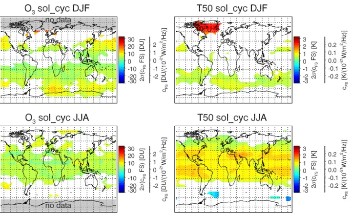
3.4 Solar cycle variations
Figure 6 shows regression results for variations attributed to the solar cycle. As usual, total ozone and 50 hPa temper-ature exhibit very similar fetemper-atures. Generally, total ozone and 50 hPa temperature are higher during solar maxima and lower during solar minima. The differences typically reach 5 to 25 DU or 0.5 to 2.5 K. Interestingly, variations are smaller in the tropics than in the extra-tropics. The largest variation is found in DJF over parts of the Arctic (red area near Green-land), and in SON over parts of the Antarctic (not shown). Note that very similar results are found, when only solar cy-cle, QBO and linear trend are allowed as explanatory vari-ables in Eq. (1), and the other explanatory varivari-ables are not used.
As pointed out by Labitzke and van Loon (2000), or Ruzmaikin and Feynman (2002), atmospheric variations at-tributed to the 11-year solar cycle differ between westerly and easterly phases of the QBO. To account for this, regres-sion was also done separately for two subsets of the data. One subset contains only data during times of westerly equa-torial zonal wind, the other subset only during easterly winds (at 50 hPa). Because of splitting into two subsets, the QBO explanatory variable must be omitted in Eq. (1). Note that
Fig. 6. Same as Fig. 4, but for total ozone fluctuations associated with the 11-year solar cycle. The scales on the false color bars give 2 standard deviations (2σ ) of the solar cycle term cF SF S in Eq. (1).The second scales give the size of the solar cycle regression coefficient
cF S. Yellow and red colors indicate positive correlation between total ozone and solar flux.
following Labitzke and van Loon, 50 hPa winds were used to separate easterly and westerly phases of the QBO, whereas throughout the rest of the paper 30 hPa winds, typically 4 months ahead of 50 hPa winds, are used as the reference. For improved clarity, we also decided to lower the confidence level to 80%, and to show only results for a regression where polar vortex strength, and of course QBO, were not included as explanatory variables. Thus, the results presented here are compatible with most of Labitzke’s investigations. Note that results outside of the polar regions change very little, when the full set of explanatory variables, including zonal winds at 60◦N and 60◦S, is used. Also, results for 50 hPa temperature change very little when the full 1958 to 2001 period is used, instead of the normal 1979 to 2001 period of TOMS/SBUV data.
Figures 7 and 8 show results for the two QBO sub-sets. As might be expected, solar cycle variations found for the com-plete data-set without grouping (Fig. 6) are similar to the av-erage of the variations found for the two sub-sets (Figs. 7 and 8). However, the solar variation is substantially larger dur-ing easterly QBO phases, and is much smaller durdur-ing west-erly phases. At low to mid-latitudes, variations are large and similar in both hemispheres during QBO-East, whereas they are generally weaker, particularly in the winter hemisphere during QBO-West. While SON (not shown) shows a
simi-lar picture as DJF, variations during MAM (not shown) are quite different from both DJF and JJA. The MAM variations are quite weak and mostly restricted to high latitudes, during QBO-East, whereas during QBO-West they are strong and similar to, but weaker than, the DJF variations for QBO-East. From the tropics to mid-latitudes, up to 40◦ or 50◦, and for both QBO subsets, the solar cycle variations are more or less zonally symmetric. High latitude variations attributed to the solar cycle, however, are not zonal, but localized to cer-tain longitudes. This is similar to the findings for the QBO in Figs. 4 and 5. Where total ozone data are available, they show similar high latitude features as 50 hPa temperature. Between QBO-East and QBO-West, the high latitude vari-ations appear at complementary longitudes: For QBO-West and DJF, 50 hPa temperatures are higher during solar max-ima over Europe, and lower over the Northern Pacific (red and blue regions in Fig. 8). For QBO-East and DJF, 50 hPa temperatures are lower during solar maxima over parts of Northern Russia and higher in the North Pacific Region (blue and red areas in Fig. 7). A complementary picture is also seen for JJA in the Southern Hemisphere. There, 50 hPa temper-atures are higher during solar maxima in a region south of South America during QBO-East, but are lower during solar maxima over the Southern Pacific during QBO-West.
Fig. 7. Same as Fig. 6, but only data during the easterly phase of the QBO (at 50 hPa) are used. To improve clarity for this figure, as well as for Fig. 8, the confidence level was reduced to 80%, and zonal winds at 60◦N and 60◦S were not included as explanatory variables.
These results for total ozone and 50 hPa temperature are broadly consistent with previous results for stratospheric temperatures or total ozone (Zerefos et al., 1997; Hood, 1997; Labitzke and van Loon, 2000). In particular it is con-firmed that variations related to the solar cycle differ from season to season and differ between westerly and easterly phases of the QBO (Labitzke and van Loon, 2000; Ruz-maikin and Feynman, 2002). As pointed out by Lee and Smith (2003), regression on data spanning only a few so-lar cycles probably cannot separate QBO and soso-lar cycle ef-fects completely. Conceptual models indicate that QBO and solar cycle can interact with atmospheric noise to change the probability for warm or cold stratospheric winters (Lawrence et al., 2000). According to Hood (1997), observed changes in lower stratospheric dynamics can explain the total ozone fluctuations and their similarity to the temperature fluctua-tions. However, general circulation models even including a representation of atmospheric chemistry, largely have not been able to reproduce the full size of the variations observed in the lower stratosphere (Labitzke et al., 2002; Tourpali et al., 2003), particularly at higher latitudes. A deeper under-standing of the underlying physical mechanisms is still lack-ing.
3.5 Stratospheric aerosol variations
Since the beginning of regular stratospheric weather records, three major volcanic eruptions, Mt. Pinatubo in 1991, El Chich´on in 1982, and Agung in 1963, have resulted in large increases of stratospheric aerosol. Most of the vol-canic aerosol leaves the stratosphere through sedimentation within about 2 to 3 years. Light absorption and scattering by the additional particles tends to warm the lower latitude stratosphere. Particularly at cold temperatures and higher lat-itudes, the particles also provide surface area for chemical re-actions, which result in enhanced ozone destruction by chlo-rine. This was most pronounced for the Pinatubo episode, when stratospheric chlorine loading was higher than at the time of the other eruptions (Solomon, 1999; Robock, 2000). Based on the 1979 to 1995 total ozone record, Solomon et al. (1996) and McCormack et al. (1997) pointed out that it may be difficult to separate between effects of the 11-year solar cycle and effects from volcanic aerosol, since both ma-jor volcanic eruptions of El Chich´on in 1982 and Pinatubo in 1991 occurred near solar maximum. Extension of the data record to 2001, almost to the next solar maximum and with-out another volcanic eruption, seems to have alleviated this problem. In the present study, nearly the same results are obtained for stratospheric aerosol related variations of total ozone and 50 hPa temperature, whether the solar-cycle is
Fig. 8. Same as Fig. 7, but for the westerly phase of the QBO (at 50 hPa). To improve clarity for this figure, as well as for Fig. 7, the confidence level was reduced to 80%, and zonal winds at 60◦N and 60◦S were not included as explanatory variables.
included in the regression or not. Similarly, results for the stratospheric solar-cycle predictor do not depend much on whether the aerosol term is included or not. Also, 50 hPa temperature variations attributed to the stratospheric aerosol term or the solar cycle term change very little when the much longer 1958 to 2001 data-set is used.
The maximum ozone and 50 hPa temperature changes attributed to stratospheric aerosol loading are shown in Fig. 9 for northern spring (MAM) and fall (SON). Since the Mt. Pinatubo eruption resulted in the highest stratospheric aerosol loading for over 50 years, the values in Fig. 9 largely reflect anomalies from the years 1991 to 1993. Different from most other explanatory variables, there is little geo-graphical correlation between the aerosol responses for total ozone and 50 hPa temperature. Temperatures at 50 hPa re-sponded by an increase, typically by 2 to over 3 K, in a broad belt between 40◦S and 40◦N. The response is very similar for all seasons. At higher latitudes, red areas in Fig. 9 above North America and south-east of Australia in SON give in-dications for strengthening and/or eastward movement of the Aleutian and Australian stratospheric anti-cyclones. Similar high-latitude features are also seen in winter in the respec-tive hemispheres (DJF and JJA, both not shown). There is no indication of a significant negative temperature response at mid-latitudes.
In contrast to 50 hPa temperature, the ozone response is usually negative. It is largest at high latitudes, smallest in the tropics. Ozone decreases exceeding 40 DU are found at northern mid to high latitudes in spring (MAM) and over parts of Antarctica in southern spring (SON). The ozone re-sponse for DJF (not shown) is very similar to MAM. In JJA (not shown) losses are found at lower latitudes like in SON, and the large northern high-latitude losses from MAM re-main, but are substantially reduced.
The aerosol responses found here, a 50 hPa temperature increase by up to 3 K at low latitudes, and total ozone deple-tions by up to 40 DU, mostly at northern high-latitudes, are consistent with previous studies (Angell , 1997; McCormack et al., 1997; Robock, 2000).
3.6 Zonal wind anomalies at 60◦N and 60◦S, 50 hPa
The intensity of the meridional residual Brewer-Dobson cir-culation in the winter stratosphere is highly correlated with the strength of the polar winter vortex (Staehelin et al., 2001; Salby and Callaghan, 2002). A stable winter vortex is also a prerequisite for large-scale chemical processing on polar stratospheric cloud particles leading to “ozone-hole” condi-tions (Solomon, 1999). Zonal wind anomalies at 60◦latitude at the 50 hPa level are a good indicator of vortex strength and were added to the set of explanatory variables. The size of
Fig. 9. Same as previous figures, but showing ozone and 50 hPa temperature changes attributed to stratospheric aerosol from the El Chich´on and Pinatubo eruption. Here the maximum positive or negative deviation of cAAis shown, not two standard deviations as in the other plots. Note also, that the scale for cAon the right is only approximate, because the aerosol data A vary with latitude.
total ozone and 50 hPa temperature fluctuations attributed to zonal wind anomalies is shown in Figs. 10 and 11 for north-ern and southnorth-ern spring.
For high winds and a strong polar vortex, total ozone and temperatures are low in the polar region. The polar varia-tions are very large and reach up to 50 DU or 5 K. Polar total ozone and 50 hPa temperature are inversely correlated to zonal wind. An opposite variation is found at mid- to low latitudes. The temperature variation is larger and is found at higher latitudes than for total ozone. Temperature variations peak at up to 2.5 K around 30◦to 40◦. Total ozone variations are more restricted to the tropics and reach up to 5 DU. The Southern Hemisphere variations (SON) are slightly weaker, but more spread out, than in the Northern Hemisphere. Re-sults for northern fall and winter (SON and DJF, both not shown) are very similar to northern spring (MAM). However, variations attributed to southern vortex strength in southern fall and winter (MAM and JJA, both not shown), are much less pronounced than in southern spring (SON). This reflects the much stronger and less variable Antarctic vortex and the generally weaker Brewer-Dobson circulation in the Southern Hemisphere during winter.
These variations of total ozone and 50 hPa temperature re-flect the close coupling of mean meridional Brewer-Dobson
circulation and polar vortex strength. A strong vortex goes hand in hand with a weak meridional circulation. Less ozone and heat are transported polewards. Total ozone and temper-atures remain high at lower latitudes and low at higher lati-tudes. A strong and cold vortex also favors rapid chemical ozone destruction in spring (“ozone hole”), which will result in low total ozone and, through less ozone radiative heating, also lower 50 hPa temperatures. This effect will enhance the transport effect. It is more relevant for the Northern Hemi-sphere where “ozone hole” conditions only occur in some years, than for the Southern Hemisphere, where a strong and stable vortex is established in almost every year.
3.7 ENSO
The El Ni˜no/Southern-Oscillation phenomenon (ENSO) is a coupled fluctuation of the tropical Pacific Ocean and the at-mosphere (e.g. Coghlan, 2002). During the El Ni˜no warm-phase, ocean surface temperature in the Eastern Tropical Pa-cific is 1 to 2 K above normal, during the La Ni˜na cold-phase it is 1 to 2 K below normal. These changes in sea sur-face temperature are accompanied by changes in many atmo-spheric parameters, e.g. tropoatmo-spheric winds and rainfall pat-terns. During El Ni˜no, tropical easterlies weaken, dry condi-tions are found in the Western Pacific (Australia, Indonesia),
Fig. 10. Same as previous figures, but showing variations related to polar vortex strength, which is represented by zonal wind anomalies at 60◦N, 50 hPa.
Fig. 11. Same as Fig. 10, but for zonal wind anomalies at 60◦S, 50 hPa.
wet conditions extend further into the Eastern Pacific (South America). The warmer sea surface temperatures also lead to a warmer troposphere and a higher tropopause throughout most of the tropics, but particularly over the Eastern Tropi-cal Pacific. In the extra tropics, particularly over regions in Eastern Asia and the Pacific, temperatures and tropopause height are lower (Kiladis et al., 2001). The opposite is the case for La Ni˜na. ENSO is accompanied by residual circu-lation cells with descending and ascending branches in the troposphere. These are compensated by opposing motions in the lower stratosphere (Gettelman et al., 2001; Kiladis et al., 2001). ENSO thus leads to lower stratospheric temperature and total ozone anomalies, that are opposite to the tempera-ture anomalies in the troposphere.
Figure 12 shows the typical size of total ozone and 50 hPa temperature changes found between La Ni˜nas and El Ni˜nos for DJF. Note that the ENSO explanatory variable used here (NCEP’s Southern Oscillation Index) is positive for La Ni˜na events and negative during El Ni˜nos. Thus, Fig. 12 shows that total ozone and 50 hPa temperature are high in DJF during La Ni˜na throughout parts of the tropics, particularly above the Eastern Pacific and the tropical Atlantic for total ozone. In the tropics, the difference between La Ni˜na and El Ni˜no is typically about 5 to 10 DU or 0.5 to 1 K. The
differences are largest in DJF and above the Eastern Pacific. SON and MAM (both not shown) exhibit similar, generally weaker and less significant, variations. A similar tropical
ENSO-related variation, i.e. zonal changes up to 10 DU with
a superimposed see-saw between the Eastern and Western Pacific, has been reported, e.g. by Shiotani (1992). Outside of the tropics, total ozone and 50 hPa temperature are gen-erally low during La Ni˜na, and high during El Ni˜no. This is most pronounced in the summer hemisphere (DJF and JJA, the latter is not shown).
A striking, zonally asymmetric, feature are the substan-tially colder 50 hPa temperatures found during La Ni˜na over Eastern Asia (−3 K, blue region in Fig. 12). They seem to be coupled to warmer temperatures over Europe (+3 K, red region). A positive anomaly over Europe is also found for total ozone. However, the strong temperature anomaly over Eastern Asia does not appear in the total ozone response, or is not significant there. The temperature anomalies indicate a weakening of the westerly part of the Aleutian anti-cyclone. This might be related to a generally stronger and more stable Arctic polar vortex during La Ni˜na (Labitzke and van Loon, 1999). As before for QBO and solar cycle, a strong polar signal from ENSO is likely taken over by the zonal wind at 60◦explanatory variable.
Fig. 12. Same as previous figures, but showing the influence of El Ni˜no/Southern-Oscillation on total ozone and 50 hPa temperature. Top panels: Obtained with full set of explanatory variables, including 400 hPa temperature. Bottom panels: Reduced set of explanatory variables, without 400 hPa temperature.
As mentioned, tropospheric temperature, e.g. at 400 hPa, and El Ni˜no are highly correlated in the tropics and some other regions. When both 400 hPa temperature and an El Ni˜no explanatory variable are used in the regression, one, the other, or both may take over part of the variation. To give an indication how serious this dependence might be, Fig. 12 contrasts ENSO results for the full regression ac-cording to Eq. (1) in the upper panels, with results where
T (400) was not included as an explanatory variable in the lower panels. Differences between the two sets of explana-tory variables are generally small and occur mainly in the tropics. When 400 hPa temperature is included (upper pan-els), total ozone and temperature variations attributed to the
ENSO predictor are weaker in the tropics, particularly over
the Eastern Pacific, ENSO’s main center of action. In this region, 400 hPa temperature takes over part of the variations that otherwise would be attributed to the ENSO explanatory variable. Similar but smaller changes are found for the other seasons (not shown). Although T (400) and ENSO are an ex-ample of highly correlated explanatory variables, the results do not depend very much on whether the other explanatory variable is included or not. For other explanatory variables the effects are usually even smaller.
4 Conclusions
Multiple linear regression analysis provides a good near global picture of natural and anthropogenic contributions to interannual variations of total ozone and lower stratospheric temperature, e.g. at 50 hPa. For most explanatory variables the geographical distribution of the attributed total ozone and 50 hPa temperature variations is very similar. It appears that interannual fluctuations of both parameters are controlled to a large degree by the same physical processes. As a rule of thumb, a 10 DU change in total ozone corresponds to a 1 K change of 50 hPa temperature. The length of the 1979 to 2001 TOMS/SBUV data record makes it possible to get a fairly good separation of different contributors. Note that re-sults for 50 hPa temperature change very little when the even longer 1958 to 2001 time period is used. There may still be difficulties, e.g. separating solar cycle and QBO related variations, or variations related to both QBO and ENSO (Lee and Smith, 2003). However, our sensitivity tests indicate no major problems. Although new data have been added and the picture presented here has become more comprehensive, findings are not fundamentally different from earlier studies, where the various contributions were studied separately (Sh-iotani, 1992; McCormack et al., 1997; Zerefos et al., 1997; Labitzke and van Loon, 2000; Baldwin et al., 2001).
Table 1. Typical size of total ozone and 50 hPa temperature variations attributed to different explanatory variables X by linear regression of Eq. (1). The second and third columns give 2 standard deviations (2σ ) of the respective terms cXX, except for stratospheric aerosol A,
where the maximum ozone and temperature change (after the Pinatubo eruption) are given. The fourth and fifth column give the typical size of the regression coefficients cX
X 2σ (cXX) cX
ozone 50 hPa temperature ozone 50 hPa temperature
T R −5 to −30 DU/decade −0.5 to −1.5 K/decade T (400) 5 to 30 DU 0.5 to 3 K −3 to −12 DU/K −0.3 to −1 K/K QBO(10/30) 5 to 25 DU 0.5 to 2.5 K −0.5 to +0.7 DU/(m/s) −0.05 to +0.07 K/(m/s) F S 5 to 25 DU 0.5 to 2.5 K 0.3 to 1.5 1021 DU W/(m2H z) 0.03 to 0.15 1021 K W/(m2H z) A up to −40 DU up to +3 K −100 to −350 DU/(1/sr) 15 to 20 K/(1/sr) u(60N ) 5 to 50 DU 0.5 to 5 K +0.3 to −3 DU/(m/s) +0.05 to −0.3 K/(m/s) u(60S) 5 to 40 DU 0.5 to 4 K +0.4 to −5 DU/(m/s) +0.1 to −0.5 K/(m/s) ENSO 5 to 10 DU 0.5 to 1 K 2 to 5 DU 0.25 to 0.5 K
For the different explanatory variables, ozone and tem-perature fluctuations range from about 5 DU or 0.5 K (two standard deviations of the corresponding time series term in Eq. (1)) to 50 DU or 5 K, respectively. A summary is given in Table 1. Large variations come from the linear trend term, up to −30 DU or −1.5 K/decade, from terms related to polar vortex strength, up to 50 DU or 5 K, from tropospheric mete-orology, up to 30 DU or 3 K, or from the QBO, up to 25 DU or 2.5 K. The 11-year solar cycle, up to 25 DU or 2.5 K, or
ENSO, up to 10 DU or 1 K, are somewhat smaller
contribu-tors. A large but sporadic variation comes from stratospheric aerosol, which leads to warming up to 3 K at low latitudes and ozone depletion up to 40 DU at high latitudes. Varia-tions related to QBO, polar vortex strength, and to a lesser degree, to ENSO exhibit a clear inverse correlation between low latitudes and higher latitudes. Variations related to solar cycle or 400 hPa temperature, however, have the same sign over most of the globe.
For most explanatory variables, total ozone and 50 hPa temperature variations are zonally symmetric at low and mid-latitudes. At high latitudes, however, zonal symmetry is more the exception than the rule. For example, QBO, solar-cycle or ENSO, all related to polar vortex strength and stratospheric warmings (Labitzke and van Loon, 1999), seem to influence position and strength of the stratospheric anti-cyclones over the Aleutians and south of Australia. This indicates that lat-itudinal effects need to be considered, when trying to under-stand the physical mechanisms leading to the observed con-nections at higher latitudes (see also Callaghan and Salby, 2002). Two-dimensional models cannot resolve latitudinal structures, and this may be a major drawback. Recently, several three-dimensional global circulation models include a representation of stratospheric chemistry with feedback of the chemical species on radiative heating and cooling (Austin et al., 2003). Two such models, MA-ECHAM and ECHAM-DLR, are currently used for transient simulations. These
simulations account for source gas changes over the last 40 years, for solar-flux changes, for changing sea-surface tem-peratures, QBO and volcanic aerosol. It is planned to ana-lyze these simulations in the same fashion as has been done for the observations in this paper. Comparison between sim-ulated and observed variations should help towards a much better understanding of the underlying mechanisms.
Acknowledgements. This investigation is part of the KODYACS
project, funded under AF02000 (www.afo2000.de) by the German Ministry for Education and Research, grant ATF43. Comments and helpful suggestions by Dr. Lon Hood and anonymous reviewers are gratefully acknowledged.
References
Andrews, D. G., Holton, J. R., and Leovy, C. B.: Middle Atmo-sphere Dynamics, Academic Press, San Diego, USA, 481, 1987. Angell, J. K.: Stratospheric warming due to Agung, El Chich´on, and Pinatubo taking into account the Quasi-Biennial Oscillation, J. Geophys. Res., 102, 9479–9485, 1997.
Appenzeller, C., Weiss, A. K., and St¨ahelin, J.: North Atlantic Oscillation modulates total ozone winter trends, Geophys. Res. Lett., 27, 1134–1138, 2000.
Austin, J. A., Shindell, D., Beagley, S. R., Br¨uhl, C., Dameris, M., Manzini, E., Nagashima, T., Newman, P., Pawson, S., Pitari, G., Rozanov, E., Schnadt, C., and Shepherd, T. G.: Uncertainties and assessments of chemistry-climate models of the stratosphere, Atm. Chem. Phys., 3, 1–27, 2003.
Baldwin, M. P. and Dunkerton, T. J.: Propagation of the Arc-tic Oscillation from the stratosphere to the troposphere, J. Geo-phys. Res., 104, 30 937–30 946, 1999.
Baldwin, M. P., Gray, L. J., Dunkerton, T. J., Hamilton, K., Haynes, P. H., Randel, W. J., Holton, J. R., Alexander, M. J., Hirota, I., Horinouchi, T., Jones, D. B. A., Kinnersley, J. S., Marquardt, C., and Takahashi, M.: The Quasi-Biennial Oscillation, Rev. Geo-phys., 39, 179–229, 2001.
Bodeker, G. E., Scott, J. C., Kreher, K., and McKenzie, R. L.: Global ozone trends in potential vorticity coordinates using
TOMS and GOME intercompared against the Dobson network: 1978–1998, J. Geophys. Res., 106, 23 029–23 042, 2001. Bojkov, R. D., Bishop, L., Hill, W. J., Reinsel, G. C., and Tiao, G.
C.: A statistical trend analysis of revised Dobson Total Ozone data over the Northern hemisphere, J. Geophys. Res., 95, 9785– 9807, 1990.
Bojkov, R. D. and Fioletov, V. E.: Estimating the global ozone characteristics during the last 30 years, J. Geophys. Res., 100, 16 537–16 551, 1995.
Callaghan, P. F. and Salby, M. L.: Three-Dimensionality and forc-ing of the Brewer-Dobson circulation, J. Atmos. Sci., 59, 976-991, 2002.
Coughlan, C.: El Ni˜no – causes, consequences and solutions, Weather, 57, 209–215, 2002.
Draper, N. R. and Smith, H.: Applied Regression Analysis, Wiley-Interscience, New York, 706, 1998.
Engel, A., Schmidt, U., and McKenna, D.: Stratospheric trends of CFC-12 over the past two decades: recent observational evidence of declining growth rates, Geophys. Res. Lett., 25, 3319–3322, 1998.
Fioletev, V. E., Bodeker, G. E., Miller, A. J., McPeters, R. D., and Stolarski, R.: Global and zonal total ozone variations estimated from ground-based and satellite measurements: 1964-2000, J. Geophys. Res., 107, 4647, doi:10.1029/2001JD001350, 2002. Gettelman, A., Randel, W. J., Massie, S., Wu, F., Read, W. G., and
Russell III, J. M.: El Ni˜no as a natural experiment for studying the Tropical Tropopause Region, J. Clim., 14, 3375–3392, 2001. Harris, J. M., Oltmans, S. J., Bodeker, G. E., Stolarski, R., Evans, R. D., and Quincy, D. M.: Long-term variations in total ozone derived from Dobson and satellite data, Atmosph. Environ., 37, 3167–3175, 2003.
Holton, J. R. and Tan, H.-C.: The influence of the equatorial quasi-biennial oscillation on the global circulation at 50 mb, J. Atmos. Sci., 37, 2200–2208, 1980.
Hood, L. L.: The solar cycle variation of total ozone: Dynamical forcing in the lower stratosphere, J. Geophys. Res., 102, 1355– 1370, 1997.
Hood, L. L., Rossi, S., and Beulen, M.: Trends in lower strato-spheric zonal winds, Rossby wave breaking behavior, and col-umn ozone at northern mid latitudes, J. Geophys. Res., 104, 24 321–24 339, 1999.
J¨ager, H., Uchino, O., and Nagai, T.: Ground-based remote sensing of the decay of the Pinatubo eruption cloud at three Northern Hemisphere sites, Geophys. Res. Lett., 22, 607–610, 1995. Kiladis, G. B., Straub, K. H., Reid, G. C., and Gage, K. S.: Aspects
of interannual and intra seasonal variability of the tropopause and lower stratosphere, Q. J. Roy. Met. Soc., 127, 1961–1983, 2001. Kistler, R., Kalnay, E., Collins, W., Saha, S., White, G., Woollen, J., Chelliah, M., Ebisuzaki, W., Kanamitsu, M., Kousky, V., van den Dool, H., Jenne, R., and Fiorino, M.: The NCEP-NCAR 50-Year Reanalysis: Monthly Means, CD-ROM and Documenta-tion, Bull. Am. Met. Soc., 82, 247–267, http://wesley.wwb.noaa. gov/reanalysis.html, 2001.
Koch, G., Wernli, H., Staehelin, J., and Peter, T.: A Lagrangian analysis of stratospheric ozone variability and long-term trends above Payerne (Switzerland) during 1970–2001, J. Geophys. Res., 107, 4373, doi:10.1029/2001JD001550, 2002.
Labitzke, K. and van Loon, H.: The stratosphere: phenomena, his-tory, and relevance, Springer Verlag, Berlin, 197, 1999.
Labitzke, K. and van Loon, H.: The QBO effect on the solar signal in the global stratosphere in the winter of the Northern Hemi-sphere, J. Atmos. Solar-Terr. Phys., 62, 621–628, 2000. Labitzke, K., Austin, J., Butchart, N., Knight, J., Takahashi, M.,
Nakamoto, M., Nagashima, T., Haigh, J., and Williams, V.: The global signal of the 11-year solar cycle in the stratosphere: ob-servations and models, J. Atmos. Solar-Terr. Phys., 64, 203–210, 2002.
Lawrence, J. K., Cavidad, A. C., and Ruzmaikin, A.: The response of atmospheric circulation to weak solar forcing J. Geophys. Res., 105, 24 839–24 848, 2000.
Lee, H. and Smith, A. K.: Simulation of the combined effects of solar cycle, quasi-biennial oscillation, and volcanic forcing on stratospheric ozone changes in recent decades, J. Geophys. Res., 108, ACH 4, doi:10.1029/2001JD001503, 2003.
McCormack, J. P., Hood, L. L., Nagatani, R., Miller, A. J., Planet, W. G., and McPeters, R. D.: Approximate separation of volcanic and 11-year signals in the SBUV-SBUV/2 total ozone record over the 1979–1995 period, Geophys. Res. Lett., 24, 2729–2732, 1997.
Perlwitz, J. and Graf, H.-F.: The statistical connection between tro-pospheric and stratospheric circulation of the Northern Hemi-sphere in winter, J. Clim., 8, 2281–2295, 1995.
Ramaswamy, V., Chanin, M. L., Angell, J., Barnett, J., Gaffen, D., Gelman, M., Keckhut, P., Koshelkov, Y., Labitzke, K., Lin, J. J. R., O‘Neil, A., Nash, J., Randel, W., Rood, R., Shiotani, M., Swinbank, R., and Shine, K.: Stratospheric temperature trends: observations and model simulations, Rev. Geophys., 39, 71–122, 2001.
Randel, W. J. and Cobb, J. B.: Coherent variations of monthly mean total ozone and lower stratospheric temperature, J. Geo-phys. Res., 99, 5433–5447, 1994.
Reed, R. J.: The role of vertical motions in ozone-weather relation-ship, J. Meteor., 7, 263–267, 1950.
Reid, G. C.: Seasonal and interannual temperature variations in the tropical stratosphere, J. Geophys. Res., 99, 18 923–18 932, 1994. Robock, A.: Volcanic eruptions and climate, Rev. Geophys., 38,
191–219, 2000.
Ruzmaikin, A. and Feynman, J.: Solar influence on a major mode of atmospheric variability, J. Geophys. Res., 107, ACL 7, doi:10.1029/2001JD001239, 2002.
Sato, M., Hansen, J. E., Lacis, A., and Thomason, L. W.: Strato-spheric aerosol optical thickness, http://www.giss.nasa.gov/data/ strataer/, 2003.
Salby, M. L. and Callaghan, P. F.: Fluctuations of total ozone and their relationship to stratospheric air motions, J. Geophys. Res., 98, 2715–2727, 1993.
Salby, M. L. and Callaghan, P. F.: Interannual changes of the strato-spheric circulation: relationship to ozone and tropostrato-spheric struc-ture, J. Clim., 24, 3673–3685, 2002.
Santer, B. D., Hnilo, J. J., Wigley, M. L., Boyle, J. S., Doutriaux, C., Fiorino, M., Parker, D. E., and Taylor, K. E.: Uncertainties in the observationally based estimates of temperature change in the free atmosphere, J. Geophys. Res., 104, 6305–6333, 1999. Shiotani, M.: Annual, Quasi-Biennial and El Ni˜no-Southern
Os-cillation ENSO time-scale variations in Equatorial Total Ozone, J. Geophys. Res., 97, 7625–7633, 1992.
Solomon, S., Portmann, R. W., Garcia, R. R., Thomason, L. W., Poole, L. R., and McCormick, M. P.: The role of aerosol
varia-tions in anthropogenic ozone depletion at northern midlatitudes, J. Geophys. Res., 101, 6713–6727, 1996.
Solomon, S.: Stratospheric ozone depletion: A review of concepts and history, Rev. Geophys., 37, 275–316, 1999.
SPARC/IOC/GAW: Assessment of Trends in the Vertical Distri-bution of Ozone, SPARC Report No. 1, WMO Global Ozone Research and Monitoring Project-Report No. 44, 1998, http: //www.aero.jussieu.fr/∼sparc/SPARCReport1/.
Staehelin, J., Harris, N. R. P., Appenzeller, C., and Eberhard, J.: Ozone trends: A review, Rev. Geophys., 39, 231–290, 2001. Steinbrecht, W., Claude, H., K¨ohler, U., and Hoinka, K. P.:
Corre-lations between tropopause height and total ozone: Implications for long-term changes, J. Geophys. Res., 103, 19 183–19 192, 1998.
Steinbrecht, W., Claude, H., K¨ohler, U., and Winkler, P.: Interan-nual changes of total ozone and Northern Hemisphere circulation patterns, Geophys. Res. Lett., 28, 1191–1194, 2001.
Stolarski, R. S. and Hollandsworth Frith, S.: Combined total ozone record from TOMS and SBUV instruments, http://code916.gsfc. nasa.gov/Data services/merged/mod data.public.html, 2002. Tourpali, K., Schuurmans, C. J. E., van Dorland, R., Steil, B., and
Br¨uhl, C.: Stratospheric and tropospheric response to enhanced solar UV-radiation: A model study, Geophys. Res. Lett., 30, doi: 10.1029/2002GL016650, 2003.
Trenberth, K. E., Stepaniak, D. P., Hurrell, J. W., and Fiorino, M.: Quality of Reanalyses in the tropics, J. Clim., 14, 1499–1510, 2001.
van Loon, H. and Labitzke, K.: The signal of the 11-year solar cycle in the global stratosphere, J. Atmos. Solar-Terr. Phys., 61, 53–61, 1999.
WMO (World Meteorological Organization): Scientific Assessment of Ozone Depletion: 2002, Global Ozone Research and Moni-toring ProjectReport No. 47, 498, Geneva, http://www.wmo.ch/ web/arep/ozone.html, 2003.
Yang, H. and Tung, K. K.: On the phase propagation of extra tropi-cal Quasi-Biennial Oscillation in observational data, J. Geophys. Res., 100, 9091–9100, 1995.
Zerefos, C. S., Bais, A. F., Ziomas, I. C., and Bojkov, R. D.: On the relative importance of Quasi-Biennial Oscillation and El Ni˜no Southern Oscillation in the revised Dobson Total Ozone records, J. Geophys. Res., 97, 10 135–10 144, 1992.
Zerefos, C. S., Tourpali, K., Bojkov, B. R., Balis, D. S., Rognerund, B., and Isaksen, I. S. A.: Solar activity-total column ozone re-lationships: Observations and model studies with heterogeneous chemistry, J. Geophys. Res., 102, 1561–1569, 1997.