Three-dimensional interface modelling with two-dimensional
seismic data: the Alpine crust–mantle boundary
F. Waldhauser,* E. Kissling, J. Ansorge and St. Mueller
Institute of Geophysics, Swiss Federal Institute of T echnology, ET H Ho¨nggerberg, CH-8093 Zu¨rich, Switzerland. E-mail: [email protected]
Accepted 1998 May 8. Received 1998 April 9; in original form 1997 October 6
S U M M A R Y
We present a new approach to determine the 3-D topography and lateral continuity of seismic interfaces using 2-D-derived controlled-source seismic reflector data. The aim of the approach is to give the simplest possible structure consistent with all reflector data and error estimates. We define simplicity of seismic interfaces by the degree of interface continuity (i.e. shortest length of offsets) and by the degree of interface roughness ( least surface roughness). The method is applied to structural information of the crust–mantle boundary (Moho) obtained from over 250 controlled-source seismic reflection and refraction profiles in the greater Alpine region. The reflected and refracted phases from the Moho interface and their interpretation regarding crustal thickness are reviewed and their reliability weighted. Weights assigned to each reflector element are transformed to depth errors considering Fresnel volumes. The 2-D-derived reflector elements are relocated in space (3-D migration) and interpolation is performed between the observed reflector elements to obtain continuity of model parameters. Interface offsets are introduced only where required according to the principle of simplicity.
The resulting 3-D model of the Alpine crust–mantle boundary shows two offsets that divide the interface into a European, an Adriatic and a Ligurian Moho, with the European Moho subducting below the Adriatic Moho, and with the Adriatic Moho underthrusting the Ligurian Moho. Each sub-interface depicts the smoothest possible (i.e. simplest) surface, fitting the reflector data within their assigned errors. The results are consistent with previous studies for those regions with dense and reliable controlled-source seismic data. The newly derived Alpine Moho interface, however, surpasses earlier studies by its lateral extent over an area of about 600 km by 600 km, by quantifying reliability estimates along the interface, and by obeying the principle of being consistently as simple as possible.
Key words: Alps, crustal structure, Moho reflection, seismic modelling, seismic
resolution, topography.
and wide-angle reflected (PmP) waves from the crust–mantle
1 I N T R O D U C T I O N
boundary, and the general continuity of these phases along crustal seismic profiles, indicate that the Moho exists virtually During the past 40 years, the greater Alpine region has been
everywhere beneath continents and is generally a continuous intensively probed by controlled-source seismology (CSS)
feature (Braile & Chiang 1986). methods (see Fig. 1) and a wealth of seismic data regarding
The great interest of Earth scientists in the depth, topography the crustal structure and thickness have been accumulated.
and lateral continuity of the Moho in orogenic belts, in Refraction and reflection seismic techniques are particularly
particular, reflects the importance of this interface in crustal well suited to detect and image seismic interfaces that exhibit
balancing, rheological and geodynamic modelling, to name a significant velocity and/or impedance contrast, the prime
just a few fields of study. In addition, the reflected and refracted example of which is the Moho discontinuity (crust–mantle
Moho phases are easily identified in crustal seismic profiling boundary). The nearly universal observation of refracted (Pn)
and, therefore, serve as guides to identify less clear earlier and later phases in the record sections. Quantitative error estimates of Moho depths and topography are of great importance to * Now at: US Geological Survey, 345 Middlefield Rd, MS 977, Menlo
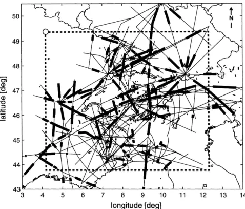
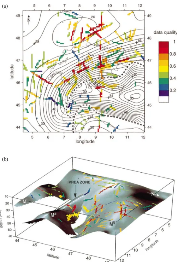
Figure 1. Seismic refraction/wide-angle reflection and near-vertical reflection profiles (thin lines) carried out over the past decades in the greater Alpine region. Superimposed are locations of 2-D-migrated Moho reflector elements (thick lines) taken from published interpretations of the controlled-source seismic profile data. The dashed box indicates the area for which the Moho interface is derived. The open circle at its NW corner facilitates orientation and comparison with Fig. 6.
Over the years, Alpine seismic data have been interpreted by region, ambiguity can be partly overcome by using structural information from nearby cross-profiles (Kissling, Ansorge & various techniques such as 1-D Herglotz–Wiechert inversion,
2-D ray-tracing methods and synthetic seismogram modelling Baumann 1997). Lateral continuity of an interface is achieved by interpolation between observed reflector data. The search to estimate the location of seismic interfaces and associated
velocities below the profile [see e.g. Egloff (1979) for 1-D for the smoothest interfaces with respect to error estimates for reflector elements requires an adequate interpolation algorithm interpretations, Aichroth, Prodehl & Thybo (1992) and Ye
et al. (1995) for 2-D interpretations]. This information has suitable to control surface roughness. Based on the principle of interface simplicity, a minimal number and length of interface usually been published as seismic cross-sections along profiles,
with very few such models including even qualitative error offsets are introduced.
The method developed for such 3-D interface modelling is estimates for derived structures (Kissling 1993). The seismic
model information, however, shows large uncertainties, mainly applied to the seismic data from the Moho in the Alpine region to derive the smoothest and laterally most continuous interface as a result of different acquisition and interpretation techniques
and the complex tectonic settings in the area of investigation. (principle of simplicity) that accounts for all 3-D-migrated data within their estimated error bounds.
Since controlled-source seismic methods are basically 2-D techniques often applied to 3-D structures (in particular true for the Alpine orogen), CSS-derived reflector elements must be
2 SE I S M I C M O H O D ATA A N D E R R O R
relocated in space (3-D migration). Before properly using the
E S T I M AT E S
2-D seismic model information for 3-D modelling, the reliability of the structural information contained in the published
2.1 Moho reflector elements
models needs to be assessed, weighted and expressed as spatial
uncertainty of the reflector-element locations. The controlled-source seismic (CSS) profile network in the greater Alpine region (Fig. 1) consists of over 200 reversed Based on 2-D seismic model information and appropriate
error estimates, a procedure is developed that searches for and unreversed wide-angle reflection and refraction profiles (in short, refraction profiles), 25 fan observations and 30 near-simplest interfaces (Waldhauser 1996). Simplicity of seismic
interfaces is defined by the degree of interface continuity and vertical reflection profiles (for overviews on the experimental activities see, e.g., Giese, Prodehl & Stein 1976; Roure, by the degree of interface roughness. The two most crucial
steps in obtaining such simplest interfaces are 3-D migration Heitzmann & Polino 1990; Meissner & Bortfeld 1990; Meissner et al. 1991; Freeman & Mueller 1992; Buness 1992 and and interpolation. While in-line migration of reflector elements
is already performed by 2-D interpretations of CSS data, off- references therein; Montrasio & Sciesa 1994; Prodehl, Mueller & Haak 1995; Ansorge & Baumann 1997; Pfiffner et al. 1997). line location of these reflector elements, however, remains
reflected phases from the Moho (PmP), which can be observed of reflector elements having a factor of 0.6 (Fig. 2). Of course, although objectivity of the weighting scheme is strived for, the on almost every wide-angle reflection profile with lengths
greater than about 100 km—depending on crustal thickness obtained weighting factors are still subjective.
By comparison with Fresnel-volume calculations for highest-and average velocity—highest-and many near-vertical reflection
pro-files, indicating that the Alpine Moho is generally a continuous quality data, the obtained total weighting factors are trans-formed into depth error estimates (Baumann 1994; Kissling feature. The PmP phases have been interpreted by 1-D and
2-D methods to determine crustal thickness. This structural et al. 1997). Considering an average frequency content of 6 Hz for Moho reflections from active sources and an average Alpine Moho information has been systematically re-evaluated and
compiled by locating the actually imaged reflecting structural Moho depth of 40 km, and assuming perfect profile design and data (w
tot=1.0), a vertical resolution frsnerr of 3 km is element (in short, reflector element) below the profile (Fig. 1).
2.2 Reflector element weighting and depth errors
The compiled Moho reflector elements show a large range of uncertainty. Data quality increased over the years with smaller shot and receiver spacings, and identification and inter-pretation of reflected phases is becoming more reliable with modern 2-D ray-tracing techniques. Furthermore, complex 3-D tectonic settings with pronounced lateral variations strongly influence the reliability of the 2-D interpretation. In this study, the information quality of reflector elements is estimated using the weighting scheme proposed by Kissling (1993) and elaborated by Baumann (1994) with separate weighting criteria for wide-angle and near-vertical reflection surveys (see Table 1). Reflector elements derived from wide-angle profiles are weighted considering raw data quality (wc) (confidence in correlation of phases), profile orientation relative to the 3-D tectonic setting (wo) and profile type (reversed or unreversed profiles, fans) (wt). Reflector elements from near-vertical reflection profiling are attributed with weights for quality of reflectivity signature (w
cr), type of migration (i.e. source of velocity used for migration) (w
mig) and projection distance (wproj, projection of subsections on to one reflection profile). Total weighting factors (w
tot) were obtained by multiplying the individual weights:
w
tot=wcwowt (refraction data) , (1)
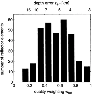
Figure 2. Distribution of weighting factors, wtot, and depth error
w
tot=wcrwmigwproj (reflection data) . (2) estimates, z
err in km, for Moho reflector elements derived from Total weighting factors between 0.1 and 1 are obtained for the controlled-source seismic profiles. Weighting factors are transformed
to depth scale using eq. (3). structural Moho data in the Alpine region, with a large number
Table 1. Weighting scheme for CSS-derived reflector elements (after Baumann 1994).
Wide-angle reflection and refraction profiles Near-vertical reflection profiles: Data quality, phase confidence (wc) Reflectivity signature (wcr):
1.0=Very confident 1.0−0.2=Confidence rate of the reflectivity signature 0.8=Confident
0.6=Likely Migration criteria (w
mig):
0.4=Poorly constrained 1.0=Migration with independent velocities from refraction
0.2=Speculative surveys
0.9=Migration with stacking velocity from reflection Profile orientation (w
c): profiles. Migration velocity model from refraction data 1.0=Along strike profiles; 0 Z alpha Z 10° projected over distances with no considerable structural 0.8=Oblique profiles; alpha>10° changes
0.8=Else Profile type, ray coverage (w
t):
1.0=Reversed refraction profile Projection criteria (w proj): 0.8=Unreversed refraction profile 1.0=Projection distance <4 km
1.0=Fan connected with reversed profile 0.9=Projection distance >4 km and <10 km 0.8=Fan connected with unreversed profile 0.8=Projection distance >10 km
derived. Based on this error estimate for the optimal case, the where z
i,jis the discrete depth value at grid node (i, j), and i
maxand jmax are the maximal grid nodes in i and j directions, weight-dependent depth uncertainty (zerr) is estimated as
respectively. Equation (4), however, allows one to compare roughness values rgh only for interfaces with equal numbers z err= frsn err w tot =±3 km w tot . (3) of nodes.
Even a large set of sampled reflector elements does not allow unique prediction of interface depths. Hence, a broad
3 3 - D S E I S M I C I N T E R FA C E M O D E L L I N G
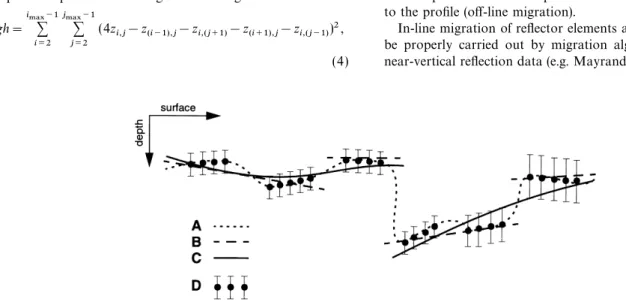
range of interpolated interfaces differing in complexity of roughness and/or continuity is possible (see Fig. 3). Assuming
3.1 Interface continuity and roughness
a set of possible interfaces that fit all reflector elements within Specific criteria have to be assumed for the process by which their uncertainties, one end of the spectrum is marked by an the Moho topography is determined based on reflector-element interface that has highest continuity, but, as a consequence, is locations and uncertainties. The simplest laterally continuous most complex in its roughness (line A in Fig. 3). The high interface is sought, with vertical offsets only when required roughness value results from the attempt to interpolate between according to predefined criteria. We define the simplicity of a large vertical offsets of some reflector elements in order to seismic interface by the degree of continuity and the degree of obtain a spatially continuous interface. The other end of the surface roughness of this interface. spectrum marks an interface with numerous vertical offsets Continuity along individual reflector elements is given by ( line B in Fig. 3). In effect, this interface consists of several correlation of regularly observed phases reflected from the same planes (sub-interfaces) that are discontinuous at those locations element of a specific seismic interface. Correlation of seismic where the corresponding interpolated interface would lie out-phases between profiles leads to the identification of reflector side the depth uncertainty. The objective here is to find the elements that belong to the same structural interface. Individual simplest interface (equally weighting continuity and roughness) reflector elements, however, do not allow the prediction of featuring highest continuity (minimal number and length of continuity between them. In the case of the crust–mantle offsets) and least roughness that fits all reflector elements boundary, vertical discontinuity (offset) occurs when this within their error limits ( line C in Fig. 3).
seismic interface is interrupted by crustal-scale thrusting or crustal block faulting. In some cases, a vertical offset between reflector elements is revealed by discontinuously observed
3.2 3-D migration
phases reflected from the same interface and along the same
Controlled-source seismic methods are often 2-D techniques profile (e.g. Ye et al. 1995). Interface offsets can be assumed
applied to 3-D structures such as the Alps and thus the when ray-traced reflector elements or reflectivity patterns show
compiled Moho reflector elements (Fig. 1) are not properly an abrupt (relative to the general roughness) change in depth
located in space. Migration is the process of restoring 3-D larger than their estimated depth errors. We quantify interface
structures from 2-D CSS-derived reflecting structural elements continuity by the length of interface offsets (i.e. shortest offset
(or reflectivity patterns). For the case of a homogeneous 2-D refers to highest continuity).
cylindrical structure (Kissling et al. 1997), reflector elements Interface roughness describes interface depth variations
from transverse CSS profiles migrate in-line along the profile relative to a smooth reference interface and is a direct measure
in the direction of the up-dipping interface (in-line migration). for the complexity of a continuous interface. We quantify
For along-strike profiles, reflector elements lie outside the interface roughness rgh by applying the 2-D finite-difference
vertical plane beneath the profile and migrate perpendicular Laplacian operator to the regular surface grid:
to the profile (off-line migration).
In-line migration of reflector elements along the profile can rgh= ∑imax−1 i=2 ∑ jmax−1 j=2 (4z
i,j−z(i−1),j−zi,(j+1)−z(i+1),j−zi,(j−1))2 , be properly carried out by migration algorithms applied to near-vertical reflection data (e.g. Mayrand, Green & Milkereit (4)
Figure 3. Types of possible interpolated interfaces (A, B and C) with varying roughness/continuity to interpolate reflector elements ( D) represented by structural depth points within their uncertainty (error bar at each structural depth point). A: Rough interface with exact data point fit. B: Straight-line interfaces that exhibit several vertical offsets (roughness zero for an individual sub-interface). C: Smooth interface that accounts for data uncertainty and shows vertical offsets when required according to the principle of interface simplicity.
1987; Holliger & Kissling 1991) or by 2-D ray-tracing methods Migration of CSS-derived reflector elements is based on the general trend of the imaged interface (migration surface) applied to wide-angle reflection data (e.g. Ye et al. 1995). 1-D
interpretation methods generally project reflector depths to in the vicinity of the reflector element. The 3-D-migration surface is obtained by an initial interpolation between the locations below the shot point (e.g. Egloff 1979). In the scope
of this work, and in areas of laterally homogeneous structures in-line migrated CSS-derived reflector elements (e.g. Fig. 1). 2-D-interpreted and, therefore, properly in-line migrated only, such 1-D-derived reflector elements have been
approxi-mately migrated in-line to half the distance of the phase reflector elements are off-line migrated perpendicular to the profile in the up-dipping direction of the initial 3-D-migration observations.
None of the above-mentioned methods provides off-line surface (see Fig. 4). 1-D-interpreted and approximately in-line migrated reflector elements are also migrated in the direction migration of the structures along individual profiles. In the
case of networked profiles, the inherent ambiguity can be of the up-dipping 3-D-migration surface. The location of the 3-D-migrated reflector element is found by searching for the overcome by using additional structural information from
nearby profiles. Off-line migration of reflector elements from ray path with incidence perpendicular to the 3-D-migration surface. The velocity in the model is assumed to be constant longitudinal profiles can be verified by in-line migrated reflector
elements from transverse crossing profiles (Ye et al. 1995). Off- (ray-theoretical migration) and, therefore, effects from intra-crustal velocity inhomogeneities on the 3-D-migration path line migration of reflector elements from oblique crossing
profiles cannot be determined exactly, since the migration are neglected.
This 3-D-migration process can be successfully applied to vector cannot be correctly separated into in-line and off-line
components. smooth interfaces such as most parts of the Moho. In the
vicinity of each reflector element, the interface can then be The case of a CSS network with perpendicular crossing
along-strike and transverse profiles to determine accurately considered as plane and the separation of the migration path is reasonable. Rough surfaces lead to migration path scattering off-line migration of in-line migrated along-strike structures is
rare. More often we have to deal with loosely networked CSS and the method applied will not be able to perform such 3-D migration properly.
profiles as in the Alpine region. For the migration process on the Alpine data, we separate the 3-D migration vector for all
reflector elements into in-line and off-line components (see 3.3 Interpolation Fig. 4). In the case of reflector elements derived from oblique
For the purpose of interpolation, reflector elements are profiles, the so-derived 3-D migration is an approximation to
discretized by a number of structural depth points sampled the real 3-D migration. Owing to the smaller weight given to
every 2 to 4 km along the individual profiles, depending on oblique profiles (see Table 1), the lateral and vertical migration
the factor with which the reflector elements are weighted. errors for these profiles will, therefore, be in the range of the
Higher weights imply higher density of structural depth points depth uncertainty of the corresponding reflector elements.
along reflector elements. A two-step procedure is applied in each interpolation process (Klingele´ 1972). In a first step, Moho depths are calculated for a coarse regular grid with a grid spacing of 18 km appropriate for the distribution and density of the observed Moho reflector elements (Fig. 1). This interpolation is carried out by least-squares fitting of poly-nomial surfaces (see e.g. Lancaster & Salkauskas 1986). Local parabolas, described by second-order polynomials, are com-puted with their apices at the grid nodes to be interpolated. Data points within a predefined radius are approximated in a least-squares procedure, weighting each data point by the inverse of the distance to the centre of the circle.
The second step includes a refining of the initial grid to a spacing of 6 km, a value similar to the estimated average horizontal resolution obtained from CSS methods for the Moho interface. It is performed by a line-by-line interpolation followed by a column-by-column interpolation on the pre-viously obtained grid, using a spline under tension whose variations of the stress factor allow an interpolation ranging from broken line to a classical bi-cubic spline (Cline 1974).
Figure 4. Map view of the 3-D migration procedure. Separation of 3-D migration vector into an in-line (1 2) and off-line (2 3)
component. An unmigrated reflector element (1) has been in-line 3.4 Procedure to derive the 3-D-migrated simplest Moho migrated by means of 2-D ray tracing. The in-line migrated reflector interface
element (2) is off-line migrated perpendicular to the profile in the
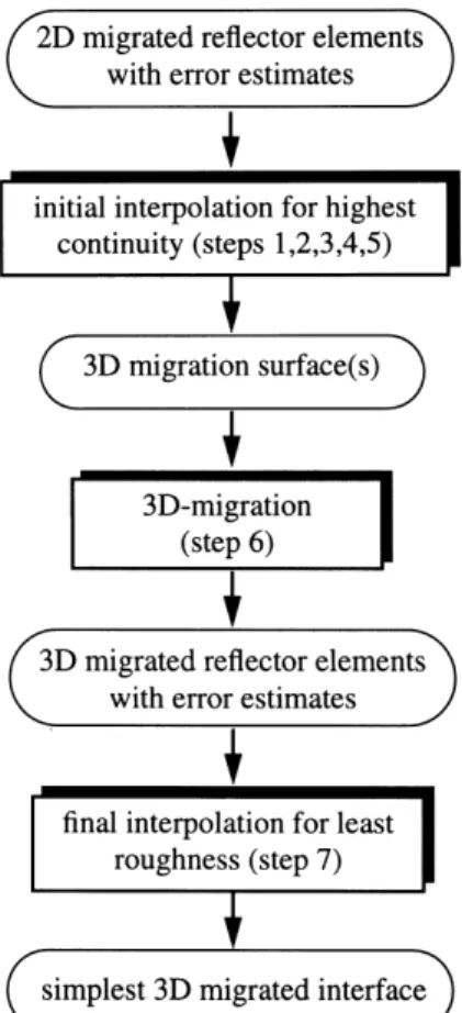
direction of updipping migration surface represented by depth isolines, The derivation of the simplest Moho interface accounting for producing the 3-D-migrated reflector element (3). The position of the all 3-D-migrated data within their error limits consists of seven 3-D-migrated reflector element is found by searching for ray paths steps (see Fig. 5).
with perpendicular incidence on the 3-D-migration surface. The
Step 1 Interpolation of 2-D-migrated and discretized Moho migration surface in the vicinity of the element to be migrated is
reflector elements (i.e. structural depth points) for single obtained by initial interpolation of reflectors belonging to the same
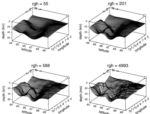
characterized by equally high continuity and differ only in their roughness. Fig. 6 gives a perspective view of four such interfaces, M
55(rgh=55, very smooth), M201, M588and M4993 (extremely rough), representing selected roughness values.
4.2 Step 2: best-fitting single interface
The quality of each interpolation, based on the variance of the misfit relative to the observation errors, and on the physical principle of interface continuity, is quantified by the root-mean-square (rms) value of the depth residuals for each interface individually: zrms=res
S
∑ kmax k=1 (Dz k)2 k max , (5) where Dzk is the difference between observed and calculated depths of the kth reflector element, and k
maxis the number of reflector elements used for interpolation.
Fig. 7 shows depth rms residuals for 14 of the 20 calculated surfaces between a roughness of 0 (plane) and 588 (rough). Solid circles indicate the three surfaces depicted in Fig. 6. Rms residuals decrease strongly from 10 km to about 3 km for increasingly rougher surfaces between rgh=0 (plane) and about rgh=201. Beyond a surface roughness of 201, rms residuals continue to decrease but only slowly to a value of
Figure 5. Process flow for 3-D interface modelling. See text for details about 2.4 km for a roughness of 588.
and description of steps 1 to 7. A ‘best-fitting’ single interface from the 20 calculated surfaces can be attached to the smallest reasonable error of ±3 km Step 2 Selection of the best-fitting single interface with (dashed line in Fig. 7), as defined previously by the optimal appropriate roughness value (see below). resolution capability of CSS methods. Interfaces with rgh>201 Step 3 Decision for continuous or discontinuous Moho show rms residuals smaller than the optimal depth error interface. (Fig. 2), and thus tend to overfit the data. These interfaces
Step 4 Introduction of the least number of necessary interface
represent unjustified rough Moho topography (see e.g. M588 offsets (i.e. separation of interfaces) based on significant misfits or M
4993in Fig. 6). Rms residuals increase rapidly for smoother between observed and calculated Moho depths (see below). surfaces with depth misfits larger than the observed typical Step 5 Interpolation for 3-D-migration surface(s) using depth error. Thus, best-fitting interpolation is achieved with the least number of necessary offsets defined by step 4 and roughness around 201.
using for each surface the lowest roughness value fitting all 2-D-migrated data within their error limits.
Step 6 3-D migration of all observed Moho reflector
4.3 Step 3: continuous or discontinuous Moho interface
elements based on individual 3-D-migration surface(s).
Step 7 Final interpolation of 3-D-migrated and discretized Fig. 8 shows the best-fitting single interface M
201 by depth Moho reflector elements from step 6 using offsets defined by contours for a zoomed area encompassing the central and step 4 (i.e. number of separated interfaces) and using for each western Alps and northern Apennines. All structural depth interface the lowest roughness value fitting all data within their points on the in-line migrated reflector elements (see Fig. 1) error limits. are used for this interpolation and are marked for the zoomed area by small grey dots in Fig. 8. No off-line migration is In the following, this procedure is applied to the crust–mantle
applied so far. In addition, structural depth points with a misfit boundary in the greater Alpine region.
to the selected interface M
201larger than the individual depth errors (significant depth misfits) are shown. Significant depth
4 T H E A L P I N E C R U S T– M A N T L E
misfits systematically above the M201 surface are represented
B O U N D A R Y by large solid circles, and those located below the M
201surface by open circles. No significant depth misfits are observed
4.1 Step 1: single-interface interpolation
outside the area shown in Fig. 8 within the greater Alpine area. The significant depth misfits remain also after 3-D A set of 20 continuous interfaces f1–20(x, y) are interpolated
migration of the 2-D-migrated reflector elements, despite the using all 165 discretized Moho reflector elements within
Figure 6. Perspective SW view of four continuous single surfaces representing the Alpine Moho with selected roughness values rgh within the range used for the initial interpolation process: M
55, M201, M588and M4993surfaces.
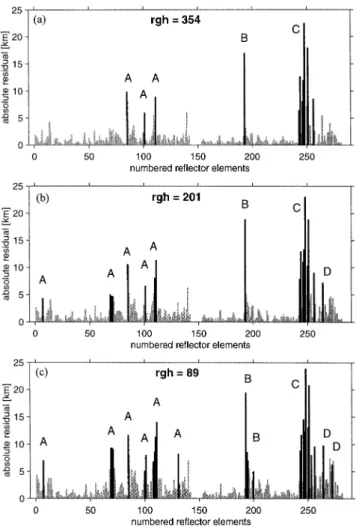
A, B, C and D label significant depth misfits that occur in the corresponding areas indicated in Fig. 8. The rougher M354 surface (Fig. 9a) still shows considerable and significant depth misfits in the south-central Alps (A) and the northern Apennines (C), where evidence for Moho offsets is given by seismic wide-angle data along the European Geotraverse (EGT) (Ye et al. 1995). Smoothing the surface to a roughness of 89 (Fig. 9c) yields increased significant depth misfits at the same location as observed on the M201 surface. The comparison shows that the best-fitting single interface M201 outlines stable localities (A, B, C, D) of significant misfit, which must represent tectonic features. At these localities, the M
201 interface is too smooth to follow the observed depths of the structural depth points within their error limits. The corresponding reflector elements lie systematically outside the interpolated interface and indicate interface offsets. Clusters of reflector elements with opposite-sign significant misfits are separated into two
Figure 7. Depth rms residuals ( km) for a set of single surfaces with ‘sub-interfaces’ (see Fig. 10). roughness rgh between 0 (plane) and 588 (very rough). The dashed
In area A (Figs 8 and 10) the European/Adriatic Moho line represents depth uncertainty for the optimal case. Solid circles
transition is characterized by the south-dipping European indicate surfaces depicted in Fig. 6.
Moho and the shallower, north-dipping Adriatic Moho. These dominant E–W-trending structural features are revealed by seismic data along the transverse near-vertical reflection
pro-4.4 Step 4: introduction of interface offsets files CT and ET (Fig. 8) (Holliger & Kissling 1991; Valasek &
Mueller 1997) and along the refraction/wide-angle reflection To avoid significant depth misfit, interface offsets have to be
profiles on the EGT (Ye et al. 1995). On the basis of depth introduced in areas such as the south-central Alps (A in Fig. 8),
error estimates for the imaged reflector elements, Baumann the northern part of the western Alps (B) and the northern
(1994) showed clear evidence for an offset between the Apennines (C and D). Before doing so, it must be shown that
two oppositely down-dipping Moho discontinuities. Thus, a the locations of these areas (A, B, C, D in Fig. 8) do not depend
WSW–ENE-striking Moho offset (bold line S
1 in Fig. 8) is strongly on the chosen surface roughness (e.g. rgh=201). Fig. 9
introduced for area A
1 that separates the European Moho shows absolute depth residuals for the M
201 surface and for
Figure 8. M201 single surface Moho (contoured at 5-km intervals) derived by interpolation of all in-line migrated and discretized reflector elements (grey dots), yielding a depth rms residual of 3 km. Significant depth misfits of points lying above (filled circles) and below (open circles) the M
201 surface are shown. Proposed Moho offsets S
1and S2are shown by bold continuous and dashed lines. Labels (e.g. LW-LC) identify CSS profiles. Figure inset shows major tectonic structures for the zoomed area (IL: Insubric Line; GL: Giudicarie Line; PL: Pustertal Line; AF: Apenninic Front). Box indicates area shown in Fig. 10. For labels A, B, C and D see text.
In area C a WNW–ESE-striking offset (bold line S
2in Fig. 8) depth is given by the significant depth misfits observed along the refraction profile LB < MC (Moho depth of about 55 km; separates the south-dipping Adriatic Moho, disappearing
beneath the Apennine front, from the shallower and slightly Ansorge 1968) and the fan profile LW N (Moho depth of about 25 km; Thouvenot et al. 1990) (see area B in Fig. 8). north-dipping Ligurian Moho. This offset is well documented
by refraction profiles along the EGT (Egger 1992; Ye et al. The proposed course of S1 between the significant depth misfits in area B is guided by the Ivrea body, an intracrustal high-1995) and along the strike of the Apennines (LW < LC,
B1 ESE; Buness 1992; Waldhauser 1996), and fan recordings density and high-velocity structure with clear association to the Adriatic crust (Schmid et al. 1987; Solarino et al. 1997). from shotpoints B1 and B2 to the east (B1 E, B2 SE;
Buness 1992). According to the spatial extension of this dominant structure (Solarino et al. 1997), offset S
1runs along its western margin As discussed above, interface offsets are first introduced in
areas A1 and C based solely on seismic information. This to the south, separating the deep European Moho from the shallow, southeast-dipping Adriatic Moho and the associated separation in both cases occurs near well-known suture zones
encompassing the Adriatic crustal block. Hence, the separation high-velocity Ivrea body. No seismic data, however, show direct evidence for continuity between the Adriatic Moho and into two interfaces is laterally continued into region B, where
seismic data are not conclusive to obtain a precise location the high velocities of the Ivrea body (Solarino et al. 1997). The south-dipping group of reflector elements (labelled LN of offset relative to these tectonic elements (the Periadriatic
tectonic Lineament; Laubscher 1983) nor to obtain the dip in Fig. 8; see Ansorge 1968) south of area B is, therefore, associated with the Adriatic Moho featuring similar dip for of the specific reflector elements. By following the Insubric
Line (IL, see Fig. 8, inset) (Schmid, Zingg & Handy 1987) this area. The exact location of S1 south of the Ivrea body, i.e. the transition between the Adriatic and European Moho in along the strike of the ESE-dipping western Alpine Moho
(Thouvenot et al. 1990; Se´ne´chal & Thouvenot 1991; Kissling this area, is not revealed by seismic data and is represented by the shortest offset length possible (dashed part of S
1), joining 1993), offset S
1 forms an arc between the European and the Adriatic Moho from location A
1in the WSW direction (Fig. 8). the Ligurian Moho (see below) at about 44.4° latitude and 7.6° longitude.
location C extends to the northwest below the LW < LC profile (location D). Such an offset improves the fit with the structural data at location D. The exact position of the triple junction where the European, the Adriatic and the Ligurian Moho join, however, is not revealed by the seismic data available. Also the southward continuation of offset S
2(i.e. the transition between the European and the Ligurian Moho) remains uncertain (dashed part of S2).
East of area C (Fig. 8), seismic data from refraction pro-file B2 SE and from fan observation B2 SW indicate a still south-dipping Adriatic Moho (Buness 1992), most likely separated from the Ligurian Moho, which continues at shallow depth (LIG74 refraction profiles; Colombi, Guerra & Scarascia 1977; Buness 1992). This is consistent with the course of the Apenninic Front (AF, see Fig. 8, inset) observed at the surface, along which offset S
2is traced to the eastern limit of the model.
4.5 Step 5: interpolation for three migration surfaces
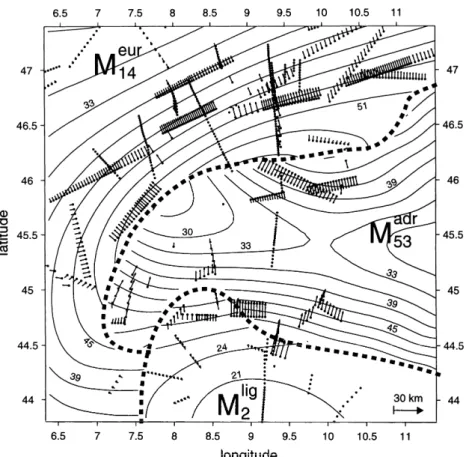
Three surfaces are obtained by opening the single interface M
201along S1and S2(see Fig. 8), i.e. separating the reflector elements along these lines and performing individual inter-polation of the European (north of S1), Adriatic (between S
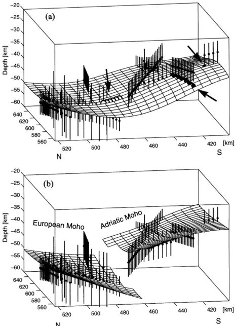
1 and S2) and Ligurian (south of S2) Moho data. Fig. 10 illustrates the effect of opening the single interface between the observed significant depth misfits using the Moho in the south-central Alps as an example (see box in Fig. 8 for location). Fig. 10(a) shows in an ESE-oriented perspective view the single M
201surface with unmigrated structural depth points and their error bars along reflector elements. Significant depth misfits are indicated by arrows on the surface. Fig. 10( b) shows the European (north) and Adriatic (south) Moho after opening the single M
201surface along S1and after individual interpolation.
Figure 9. Absolute depth residuals for single surfaces (a) M354, Numerical instabilities during interpolation at the surface ( b) M201 and (c) M89. Black bars A, B, C and D indicate areas
edges are avoided by using auxiliary depth points outside the (see Fig. 8) where significant depth misfits are observed.
surfaces where necessary, linearly extrapolating the geometry of the area near the interface edge. In areas of few (e.g. NE Po Plain; Slejko et al. 1987), unreliable or even no seismic data within the model frame, such as in the northwestern part From location A
1 (Fig. 8) to the east, only a fan profile (C2 E, see area A
2 in Fig. 8) indicates a south-dipping (eastern France), auxiliary depth points are used for interpolation that produce the simplest Moho topography consistent with European Moho and a slightly shallower, north-dipping
Adriatic Moho (Musacchio et al. 1993). The distinct significant gravity data. For example, Moho depths based on the Verona gravity high are taken into account for the eastern Po Plain depth misfit in area A2 is at least partly caused by
3-D-migration effects. Whether the transition from the European area.
Again, a set of 20 surfaces featuring a broad roughness range to the Adriatic Moho is a trough or consists of one or several
small offsets is not revealed by the available data. Still in is calculated for each of the three Mohos separately. Smoothest surfaces (migration surfaces) are sought that fit all data within accordance with the little seismic information available (see
also Fig. 1), the further continuation of S
1to the eastern limits observed depth errors, i.e. without significant depth misfit. In Fig. 11, the number of significant depth misfits is plotted against of our model follows the Periadriatic Lineament (Laubscher
1983), i.e. along the Insubric Line (IL), the NNE-wards surface roughness for each migration surface. Roughness values are chosen for the European (rgh=13.8), the Adriatic trending Giudicarie Line (GL), and along the ESE-wards
running Pustertal Line (PL) (see Fig. 8, inset). (rgh=52.6) and the Ligurian (rgh=1.9) migration surfaces (Figs 11a, b and c, respectively).
The Moho offset S
2 at location C (Fig. 8) is traced to the northwest, and merges into a south-turning arc encircling the shallow reflector elements determined from refraction profiles
4.6 Step 6: 3-D migration
LW < LC, Q NW, Q W (Buness 1992) and LN NE
(Stein, Vecchia & Froelich 1978), and from the fan profile X2 To complete 3-D migration, off-line migration of the 2-D in-line migrated reflector elements along the migration surfaces (Nadir 1988), which belong to the Ligurian Moho ( location D).
A 3-D interpretation of the LW < LC profile (Waldhauser Meur14, Madr53 and Mlig2 (Fig. 12) is subsequently performed using the method described in Section 3.2 (see also Fig. 4). Consistent et al. 1994) migrates the reflector element of the Ligurian
Moho to the south and that of the Adriatic Moho to the migration vector orientations are obtained, with a maximum horizontal displacement of about 17 km (Fig. 12). More than north, and clearly indicates that the Moho offset modelled at
Figure 10. (a) Perspective ESE-oriented view on continuous M201 surface of the Moho in the region of the south-central Alps below the Insubric Line along the EGT (see box in Fig. 8). Arrows indicate structural depth points with depth errors and significant depth misfits on the M
201 surface. ( b) Same perspective view on the Moho offset between European Moho (N) and Adriatic Moho (S) after opening the M
201surface along S
1in Fig. 8.
2 km for the vertical component of migration vectors in the
5 D I S C U S S I O N A N D C O N C L U S I ON S
northern Apennines is obtained, where the deep-reaching and
strongly dipping Adriatic Moho is mainly imaged by along- The resulting model of the Alpine Moho (Fig. 13) shows two strike profiles. Reflector elements from the European Moho offsets with three sub-interfaces: the European, the Adriatic along the Alpine longitudinal profiles migrate by about 1 km and the Ligurian Moho. Moho depths are in good accord in the vertical direction. with previous studies for those regions with dense and reliable controlled-source data (Ansorge et al. 1987; Nadir 1988; Valasek 1992; Giese & Buness 1992; Kissling 1993; Baumann
4.7 Step 7: final interpolation for three sub-interfaces 1994; Hitz 1995), and with recent studies using local earthquake
data (Solarino et al. 1997; Parolai, Spallarossa & Eva 1997). The 3-D-migrated reflector elements are used in a final
inter-The Alpine Moho interface derived in this study surpasses polation process, again selecting the three smoothest Moho
earlier studies by its lateral extent over an area of about sub-interfaces that still fit the European, the Adriatic and the
600 km by 600 km, by quantifying reliability estimates along Liguarian reflector data within the error limits, and including
the interface (see Fig. 13) and by obeying the principle of being the required interface offsets according to the principle of
The Adriatic Moho (Fig. 13) is best imaged along the EGT profile, where it is updoming below the Po Plain between the European and the Ligurian Moho. At the northern rim, the Adriatic Moho is underthrusted by the European Moho, whereas at the southern rim it is overthrusted by the Ligurian crustal block. The southern Adriatic Moho is lost at a depth of about 54 km and a further deepening cannot be determined by available 2-D controlled-source seismic methods. Further to the west, near the western margin of the Po Plain, the Adriatic Moho merges into the structure of the Ivrea zone (see Fig. 13b), where the situation again remains unclear. Strong near-surface reflections related to the Ivrea body, with phase characteristics of PmP phases, can be observed in this region (Berckhemer 1968). No seismic evidence exists for a direct contact between these near-surface reflections attributed to the high-velocity Ivrea body and the PmP reflections from the Adriatic Moho further east. The Ivrea body with its Moho-like velocity contrast is considered, however, as an intracrustal high-velocity zone (Solarino et al. 1997) associated with the Adriatic Moho. A direct contact between the Adriatic and European Moho may possibly exist below the southwestern Po Plain, where the two Mohos show a similar depth of about 48 km. The updoming eastern part of the Adriatic Moho, where no seismic data are available (see also Fig. 1), has tentatively been modelled by eastward extrapolation of the observed structure in the central part in accordance with observed gravity data (Slejko et al. 1987; Carozzo et al. 1991). The Ligurian Moho (Fig. 13) along the EGT beneath the Apennines is well located at a shallow depth of around 20 km. At its northern rim, below the front of the Apennines, the Ligurian Moho shows an offset of about 30 km relative to the deeper Adriatic Moho. West of the EGT profile, the Ligurian Moho shows possibly a slight deepening, ending below the western Po Plain. There the Ligurian Moho lies above the European Moho, separated by an offset of about 10 km. To the east of the EGT profile, the Ligurian Moho seems to continue in a shallow fashion, with unrevealed contact to the Adriatic Moho.
The obtained Alpine Moho topography reflects the present large-scale Alpine tectonic structure resulting from the collision of the African Plate with the European Plate. The two Moho offsets below the Insubric Line and below the northern Apennines confirm a southward subduction of the European
Figure 11. Number of significant depth misfits as a function of
Moho under the shallower, north-dipping Adriatic Moho, surface roughness rgh for (a) European, (b) Adriatic and (c) Ligurian
and a southward subduction of the Adriatic Moho beneath migration surfaces.
the Ligurian Moho. The Adriatic Moho is updoming below the Po Plain (see Fig. 13), most likely as the combined result of compressional forces due to the NNW-drifting African Below the central Alps the European Moho (Fig. 13) features
a south-dipping interface, deepening from 28 km below the Plate and of subduction-related loading beneath the northern Apennines.
stable foreland to more than 55 km below the Insubric Line.
This structure is well constrained by combined wide-angle and None of the presently available CSS data provide con-clusive and direct evidence that the European and the Adriatic near-vertical reflection data. A further southward continuation
of the European Moho below the Adriatic Moho, as, for lithosphere penetrate deep into the upper mantle beneath the southern Alps and the Liguarian Sea, respectively. Crustal example, proposed by Valasek (1992), has not been reliably
imaged by controlled-source seismic methods but seems balancing considerations (Pfiffner et al. 1990; Me´nard, Molnar & Platt 1991), however, suggest a continuation also of lower plausible in the light of tectonic models (Schmid et al. 1996).
The European Moho below the central Alps changes to the European crust beneath the Adriatic upper mantle south of the Insubric Line (Schmid et al. 1996). Such a subduction east-dipping arc of the western Alps. The shape of the European
Moho below the southern end of the western Alps cannot structure is also likely below the Apennines, where the Adriatic Moho underthrusts the Ligurian Moho. To resolve litho-be determined reliably litho-because of missing seismic data (see
also Fig. 1). The proposed offset between the European and spheric slab structures beneath an overriding plate, however, requires deep-seated seismic sources as are employed by local Ligurian Moho (see also S
Figure 12. Migration surfaces for the European Moho (rgh=14), the Adriatic Moho (rgh=53) and the Ligurian Moho (rgh=2) represented by depth isolines at 3-km intervals for area as in Fig. 8. Isoline values are indicated by numbers. Horizontal components of the 3-D migration vectors are marked by arrows. For migration distance in km, see reference arrow in lower right corner.
earthquake and teleseismic tomography (e.g. Spakman, Van fact that the Moho interface exists everywhere below the Alps. Accordingly, the striving for highest continuity within carefully der Lee & Van der Hilst 1993; Solarino et al. 1997).
In contrast to previous studies to derive a map of Moho determined areas as a criterion for interface simplicity is justified. In the Alpine region, Moho offsets are directly observed at topography (e.g. Buness 1992; Scarascia & Cassinis 1997), the
new technique presented in this paper aims to find the simplest only two locations below the EGT profile. The introduction of the least number of interfaces with the shortest lengths of possible interface that is consistent with all 3-D-migrated
CSS data within their previously specified error estimates. A offsets that fit all seismic data within their error limits is based on the principle of simplicity. In addition to clear Moho fundamentally different approach has, for example, been taken
by Giese & Buness (1992) and Scarascia & Cassinis (1997), who reflections from largely different depths within relatively short lateral distance, clear evidence for a Moho offset demands the obtained rather complex Moho structures with several offsets
and fragmentations that likely represent an overinterpretation a priori definition of error estimates for CSS data and 3-D migration. With respect to Moho topography in most areas, of the available data.
Moho offsets and Moho gaps in the seismic interface play our proposed weighting scheme for CSS data to obtain error estimates might seem overly detailed. To test the evidence for key roles in tectonic interpretations of 3-D crustal structure.
When interpreted as a zone of absent Moho interface (Pfiffner a Moho offset, however, we feel that all terms of the weighting scheme are necessary. For geometrical reasons and as a result et al. 1990), a gap in seismic information about the European
Moho could be interpreted as a zone of symmetric subduction of the limited number of profiles, Moho offsets are only locally imaged by CSS data. Hence, modelling the lateral extent of of lithosphere, a so-called ‘Verschluckungs’ zone (Laubscher
1970). It was shown for the Alpine region, however, that observed such a Moho offset by connecting clusters of significant depth misfits (see Fig. 8 and Step 4 in the interface modelling data gaps along near-vertical reflection profiles (Pfiffner et al.
1990) are not caused by an absent Moho interface. Holliger procedure) relies strongly on plate-tectonic and geodynamic concepts and introduces additional ambiguity to the model. & Kissling (1992) imaged the expected Moho structure
using wide-angle data from cross-profiles, and Valasek et al. The applied weighting scheme and the derived depth error estimates for seismic data are parameters that significantly (1991) imaged the Moho in the same region using wide-angle
reflections along the EGT profile (see Fig. 14). These results influence the 3-D interface modelling results. We are well aware that the weighting scheme is still subjective, although we strove obtained along the EGT transect by networked wide-angle
and near-vertical profiling and the clear evidence for Moho for as much objectivity as possible. As shown earlier in this study, altering the weighting scheme and consequently the offsets (see Figs 8 and 13), which indicate asymmetric
(a)
(b)
Figure 13. (a) Alpine Moho interface contoured at 2-km intervals derived by smoothest interpolation of the 3-D-migrated CSS data. Isoline values are indicated by numbers. The structural, 3-D-migrated database is shown by colours indicating weighting factors between 0.1 (information poorly constraint by CSS methods) and 1 (highly reliable reflectors from CSS methods) and by size of Fresnel zone on Moho interface. ( b) Perspective SW view on the Moho below the Alpine region—European (Me), Adriatic (Ma) and Ligurian (Ml) Moho.
resulting interfaces but it does not lead to significantly different quantitatively constrains the large-scale Alpine crustal structure (Fig. 13). The technique may be applied to Moho interfaces interface offsets (see Fig. 9).
The new method to derive a seismic interface topography in other regions with sufficiently dense CSS data and to other interfaces (e.g. upper/lower crust discontinuity). Such outlined in this study and applied to the Alpine Moho data
Figure 14. Summary of seismically determined 2-D main crustal structure and Moho depth along the NFP20 eastern transect (reproduced from Schmid et al. 1996). Horizontal and vertical scales are the same in both panels. (a) Migrated near-vertical reflections along the eastern traverse and generalized seismic crustal structure derived from orogen-parallel refraction profiles (Holliger & Kissling 1992). Solid lines indicate the position of the Moho, derived from orogen-parallel refraction profiles. (b) Normal-incidence representation of the wide-angle Moho reflections along the EGT refraction profiles perpendicular to the orogen ( Valasek et al. 1991). Note that the gap in the reflectivity signal from the lower crust between 35 and 65 km profile distance in (a) is clearly covered by wide-angle reflection data.
Alps: Results of NRP20, pp. 25–30, eds Pfiffner, O.A., Lehner, P., consistently parametrized interface models are reproducible,
Heitzmann, P., Mueller, St. & Steck, A., Birkha¨user Verlag, Basel. updatable and regionally extendable. Besides serving as a base
Ansorge, J., Kissling, E., Deichmann, N., Schwendener, H., Klingele´, E. for tectonic interpretation, they are well suited for their use in
& Mueller, St., 1987. Krustenma¨chtigkeit in der Schweiz aus computational processes. By integration into a 3-D velocity
Refraktionsseismik und Gravimetrie, Abstract, Nat. Forschungs-model, the Alpine Moho model has been successfully used for
programm 20 (NFP20) ‘Geologische Tiefenstruktur der Schweiz’, simulations of 3-D teleseismic wavefront distortion in the
Bull. 4, 12.
Alpine region (Waldhauser 1996), and it may also be used Baumann, M., 1994. Three-dimensional modeling of the crust– for gravity modelling by integration in a 3-D density model. mantle boundary in the Alpine region, PhD thesis, No. 10772, Furthermore, the possibility of quantitative assessment of ETH-Zu¨rich.
the reliability of a seismic model helps in designing future Berckhemer, H., 1968. Topographie des ‘Ivrea–Ko¨rpers’ abgeleitet aus experiments aimed at improving and extending the present seismischen und gravimetrischen Daten, German Research Group for Explosion Seismology, Schweiz. Mineral. Petrogr. Mitt., 48, knowledge about the Alpine crust–mantle boundary.
235–246.
Braile, L.W. & Chiang, C.S., 1986. The continental Mohorovicic
A C K N O W L E D G M E N T S discontinuity: results from near-vertical and wide-angle seismic
reflection studies, in Reflection Seismology: A Global Perspective, We wish to thank M. Bopp (Mu¨nchen) and E. Flu¨h (Kiel ) for
pp. 257–272, eds Barazangi, M. & Brown, L., Geodynamics Series, their thorough and constructive reviews. One of the authors
13, Am. Geophys. Union, Washington, DC.
(FW) was supported for a PhD thesis by stipends from Kanton
Buness, H., 1992. Krustale Kollisionsstrukturen an den Ra¨ndern Basel and from ETH Zu¨rich. der nordwestlichen Adriaplatte, Berliner Geowissenschaftliche
Abhandlungen, 18, Reihe B, FU Berlin.
Carrozzo, M.T., Luzio, D., Margiotta, C. & Quarta, T., 1991. Gravity
R E F E R E N C E S
map of Italy, in Structural Model of Italy and Gravity Map, ed. Scandone, P., quaderni de ‘La Ricerca Scientifica’ 114/3, CNR, Aichroth, B., Prodehl, C. & Thybo, H., 1992. Crustal structure along
Rome. the Central Segment of the EGT from seismic-refraction studies,
Cline, A.K., 1974. Scalar and planar curve fitting using spline under T ectonophysics, 207, 43–64.
tension, Commun. ACM, 17 (4), 218–220. Ansorge, J., 1968. Die Struktur der Erdkruste an der Westflanke der
Colombi, B., Guerra, I. & Scarascia, S., 1977. Crustal structure along Zone von Ivrea, Schweiz. Mineral. Petrogr. Mitt., 48, 247–254.
two seismic refraction lines in the Northern Apennines ( lines 1b Ansorge, J. & Baumann, M., 1997. Acquisition of seismic refraction
Egger, A., 1992. Lithospheric structure along a transect from the Pfiffner, O.A., Frei, W., Valasek, P., Sta¨uble, M., Levato, L., DuBois, L., Schmid, S.M. & Smithson, S.B., 1990. Crustal shortening Northern Apennines to Tunisia derived from seismic refraction data,
in the Alpine orogen: results from deep seismic reflection profiling PhD thesis, No. 9675, ETH-Zu¨rich.
in the eastern Swiss Alps, line NFP20-east, T ectonics, 9/6, Egloff, R., 1979. Sprengseismische Untersuchungen der Erdkruste in
1327–1355. der Schweiz, PhD thesis, No. 6502, ETH Zu¨rich.
Pfiffner, O.A., Lehner, P., Heitzmann, P., Mueller, St. & Steck, A. Freeman, R. & Mueller, St. (eds), 1992. Atlas of compiled data, in A
(eds), 1997. Deep Structure of the Swiss Alps: Results of NRP20, continent revealed: T he European Geotraverse, eds Blundell, D.,
Birkha¨user Verlag, Basel. Freeman, R. & Mueller, St., Cambridge University Press, Cambridge.
Prodehl, C., Mueller, St. & Haak, V., 1995. The European Cenozoic Giese, P. & Buness, H., 1992. Moho depth, in Atlas of compiled data,
rift system, in Continental Rifts: Evolution, Structure, T ectonics, pp. 11–13, eds Freeman, R. & Mueller, St., in A continent revealed:
pp. 133–212, ed. Olson, K.H., Elsevier, Amsterdam. T he European Geotraverse, eds Blundell, D., Freeman, R. &
Roure, F., Heitzmann, P. & Polino, R. (eds), 1990. Deep Structure of Mueller, St., Cambridge University Press, Cambridge.
the Alps, Vol. spec. Mem. Soc. geol. France, Paris, 156; Mem. Soc. Giese, P., Prodehl, C. & Stein, A. (eds), 1976. Explosion Seismology in
geol. Suisse, Zu¨rich, 1; Soc. geol. Italia, Rome, 1. Central Europe, Springer-Verlag, Berlin.
Scarascia, S. & Cassinis, R., 1997. Crustal structures in the central-Hitz, L., 1995. The 3D crustal structure of the Alps of eastern eastern Alpine sector: a revision of the available DSS data,
Switzerland and western Austria interpreted from a network of T ectonophysics, 271, 157–188.
deep-seismic profiles, T ectonophysics, 248, 71–96. Schmid, S.M., Zingg, A. & Handy, M., 1987. The kinematics of Holliger, K. & Kissling, E., 1991. Ray-theoretical depth migration: movements along the Insubric Line and the emplacement of the
methodology and application to deep seismic reflection data across Ivrea Zone, T ectonophysics, 135, 47–66.
the eastern and southern Swiss Alps, Eclogae Geol. Helv., 84/2, 369–402. Schmid, S.M., Pfiffner, O.A., Froitzheim, N., Scho¨nborn, G. & Holliger, K. & Kissling, E., 1992. Gravity interpretation of a unified Kissling, E., 1996. Geophysical–geological transect and tectonic
2D acoustic image of the central Alpine collision zone, Geophys. evolution of the Swiss–Italian Alps, T ectonics, 15/5, 1036–1064. J. Int., 111, 213–225. Se´ne´chal, G. & Thouvenot, F., 1991. Geometrical migration of line-Kissling, E., 1993. Deep structure of the Alps—what do we really drawings: a simplified method applied to ECORS data, in Continental L ithosphere: Deep Seismic Reflections, pp. 401–407, know? Phys. Earth planet. Inter., 79, 87–112.
eds Meissner, R., Brown, L., Du¨rbaum, H.J., Franke, W., Fuchs, K. Kissling, E., Ansorge, J. & Baumann, M., 1997. Methodological
& Seifert, F., Geodynamics Series, 22, Am. Geophys. Union, considerations of 3-D crustal structure modeling by 2-D seismic
Washington, DC. methods, in Deep Structure of the Swiss Alps: Results of NRP20,
Slejko, D., et al., 1987. Modello Sismotettonico dell’Italia Nord-pp. 31–38, eds Pfiffner, O.A., Lehner, P., Heitzmann, P., Mueller, St.
Orientale, Consiglio Nazionale delle Ricerche, Gruppo Nazionale & Steck, A., Birkha¨user Verlag, Basel.
per la Difesa dai Terremoti, Rendiconto no. 1, Trieste, Italy. Klingele´, E., 1972. Contribution a` l’e´tude gravime´trique de la
Solarino, S., Kissling, E., Sellami, S., Smriglio, G., Thouvenot, F., Suisse Romande et des re´gions avoisinantes, Mate´riaux pour la
Granet, M., Bonjer, K.P. & Sleijko, D., 1997. Compilation of a Ge´ologie de la Suisse, Se´rie Ge´ophysique, 15, Ku¨mmerly & Frey,
recent seismicity data base of the greater Alpine region from several Geographischer Verlag, Bern.
seismological networks and preliminary 3D tomographic results, Lancaster, P. & Salkauskas, K., 1986. Curve and Surface Fitting,
Ann. Geofis., XL, 1, 161–174. Academic Press, New York.
Spakman, W., Van der Lee, S. & Van der Hilst, R., 1993. Travel-time Laubscher, H.P., 1970. Bewegung und Wa¨rme in der Alpinen tomography of the European–Mediterranean mantle down to
Orogenese, Schweiz. Mineral. Petrogr. Mitt., 50, 565–596. 1400 km, Phys. Earth planet. Inter., 79, 3–74.
Laubscher, H.P., 1983. The late Alpine (Periadriatic) intrusions and Stein, A., Vecchia, O. & Froelich, R., 1978. A seismic model of a the Insubric Line, Mem. Soc. Geol. It., 26, 21–30. refraction profile across the western Po valley, in Alps, Appenines, Mayrand, L.J., Green, A.G. & Milkereit, B., 1987. A quantitative Hellenides, pp. 180–189, eds Closs, H., Roeder, D. & Schmidt, K.,
approach to bedrock velocity resolution and precision: the Schweizerbart Verlag, Stuttgart.
LITHOPROBE Vancouver Island experiment, J. geophys. Res., 92, Thouvenot, F., Paul, A., Se´ne´chal, G., Hirn, A. & Nicolich, R., 1990.
4837–4845. ECORS–CROP wide-angle reflection seismics: constraints on deep
Meissner, R. & Bortfeld, R.K. (eds), 1990. Dekorp-Atlas, Springer- interfaces beneath the Alps, in Deep Structure of the Alps, pp. 97–106, Verlag, Berlin. eds Roure, F., Heitzmann, P. & Polino, R., Vol. spec. Mem. Soc. geol. France, Paris, 156; Mem. Soc. geol. Suisse, Zu¨rich, 1; Soc. Meissner, R. and the DEKORP Research Group, 1991. The DEKORP
geol. Italia, Rome, 1. survey: major achievements for tectonical and reflective styles, in
Valasek, P., 1992. The tectonic structure of the Swiss Alpine crust Continental L ithosphere: Deep Seismic Reflections, pp. 69–76, eds
interpreted from a 2D network of deep crustal seismic profiles and Meissner, R., Brown, L., Du¨rbaum, H.J., Franke, W., Fuchs, K.
an evaluation of 3D effects, PhD thesis, No. 9637, ETH-Zu¨rich. & Seifert, F., Geodynamics Series, 22, Am. Geophys. Union,
Valasek, P. & Mueller, St., 1997. A 3D tectonic model of the central Washington, DC.
Alps based on an integrated interpretation of seismic refraction and Me´nard, G., Molnar, P. & Platt, J.P., 1991. Budget of crustal shortening
NRP20 reflection data, in Deep Structure of the Swiss Alps: Results and subduction of continental crust in the Alps, T ectonics, 10/2,
of NRP20, pp. 305–325, eds Pfiffner, O.A., Lehner, P., Heitzmann, P., 231–244.
Mueller, St. & Steck, A., Birkha¨user Verlag, Basel. Montrasio, A. & Sciesa, E. (eds), 1994. Proceedings of Symposium
Valasek, P., Mueller, St., Frei, W. & Holliger, K., 1991. Results of NFP 20 ‘CROP—Alpi Centrali ’, Sondrio, 20–22 October 1993, Quad.
seismic reflection profiling along the Alpine section of the European Geodynamica Alpina e Quat., Milano.
Geotraverse (EGT), Geophys. J. Int., 105, 85–102.
Musacchio, G., De Franco, R., Cassinis, R. & Gosso, G., 1993. Waldhauser, F., 1996. A parametrized three-dimensional Alpine crustal Reinterpretation of a wide-angle reflection ‘fan’ across the Central model and its application to teleseismic wavefront scattering, PhD Alps, J. appl. Geophys., 30, 43–53. thesis, No. 11940, ETH-Zu¨rich.
Nadir, S., 1988. Structure de la crouˆte continentale entre les Waldhauser, F., Kissling, E., Baumann, M. & Ansorge, J., 1994. 3D Alpes Occidentales et les Alpes Ligures et ondes S dans la crouˆte seismic model of the crust under the central and western Alps continental a` l’ouest du Bassin de Paris, PhD thesis, University of (Abstract), European Geophysical Society, XIX General Assembly,
Paris VII. Grenoble, Ann. Geophys., 12, Suppl. I, C23.
Parolai, S., Spallarossa, D. & Eva, C., 1997. Lateral variations of P
n Ye, S., Ansorge, J., Kissling, E. & Mueller, St., 1995. Crustal structure wave velocity in northwestern Italy, J. geophys. Res., 102 (B4), beneath the eastern Swiss Alps derived from seismic refraction data,
T ectonophysics, 242, 109–221. 8369–8379.