BEHAVIORAL AND BRAIN SCIENCES (1990) 13, 109-161 Printed in the United States of America
Douglas Wahlsten*
Department of Psychology, University of Alberta, Edmonton, Alberta, Canada T6G2E9
Electronic mail: [email protected]
Abstract? It makes sense to attribute a definite percentage of variation in some measure of behavior to variation in heredity only if the effects of heredity and environment are truly additive. Additivity is often tested by examining the interaction effect in a two-way analysis of variance (ANOVA) or its equivalent multiple regression model. If this effect is not statistically significant at the a = 0.05 level, it is common practice in certain fields (e.g., human behavior genetics) to conclude that the two factors really are additive and then to use linear models, which assume additivity. Comparing several simple models of nonadditive, interactive relationships between heredity and environment, however, reveals that ANOVA often fails to detect nonadditivity because it has much less power in tests of interaction than in tests of main effects. Likewise, the sample sizes needed to detect real interactions are substantially greater than those needed to detect main effects. Data transformations that reduce interaction effects also change drastically the properties of the causal model and may conceal theoretically interesting and practically useful relationships. If the goal of partitioning variance among mutually exclusive causes and calculating "heritability" coefficients is abandoned, interactive relationships can be examined more seriously and can enhance our understanding of the ways living things develop.
Keywords? causal models; gene action; heritability; nature/nurture; power; sample size; scale transformation
The statistical analysis of data helps the researcher detect consistent patterns of results that might otherwise be obscured by uncontrolled and unknown sources of varia-tion. Like every analytical technique, a statistical method is based on certain assumptions about the properties of the objects being studied. If assumptions are not valid, the method can lead to erroneous conclusions just as readily as can a faulty laboratory procedure. A method can be used with confidence only if there are effective ways to test its validity. As discussed by Grusio (in press), certain experimental designs do not lend themselves to tests of crucial assumptions, no matter how many obser-vations are made. Another difficulty, the focus of this target article, arises when a test is possible, at least in principle, but is so insensitive that violations of assump-tions often escape detection.
The widespread application of the analysis of variance (ANOVA) to factorial experiments in the behavioral and brain sciences provides a case in point. This technique, first devised by Fisher and Mackenzie (1923) for use in agriculture, is convenient for evaluating the results of an experiment in which every category of one factor (e.g., variety of a crop species) is combined with every condi-tion of another factor (e.g., kind or amount of fertilizer). The classical ANOVA method is gradually being replaced by a more flexible technique, multiple regression, which fits data to a linear equation with one term for each
separate "effect" in the experiment, but for simple fac-torial designs the two procedures are essentially the same (Edwards 1979). ANOVA partitions the total variation in a measure (e.g., crop yield) among four contributing causes: (a) the "main" effect of variety averaged over all kinds of fertilizer, (b) the main effect of fertilizer averaged over all varieties, (c) the "interaction" of variety and fertilizer, and (d) sources of variation or "error" within each group. Interaction in a factorial experiment signifies the departure of a group mean score from the simple sum of the respective main effects. If present, it indicates that crop yield depends on the specific combination of variety and treatment. One of the great merits of the ANOVA method is that it can readily detect interaction. Unfortu-nately, the technique is relatively insensitive to certain types of interaction and can be quite misleading when interpreted uncritically.
Many psychological theories rise or fall with the occur-rence or absence of statistical interaction. Discussing the question of whether or not drive and reinforcement are independent, Mackintosh (1974) wrote: "In principle, the question should be answered easily, requiring no more than a large factorial experiment in which several levels of drive are combined with several magnitudes of reinforcement, with an analysis of variance being per-formed to test for a significant interaction of the two factors" (p. 154). Another example is the "person-situa-tion" question. Psychologists ask whether an individual has a distinct personality, which remains the same in a
Wahlsten: Heredity-environment interaction
variety of situations (relative stability), or whether per-sonality is highly flexible and specific to circumstance (situationism). It could also happen that personality changes according to the situation but that the kind of change depends on stable characteristics of the person (coherence). Rival explanations such as relative stability and coherence are often contrasted using AN OVA. Mag-nusson and Allen (1983) state: "Though most of the variance in a Person X Situation matrix of data is usually because of the main effects of persons, enough variance is left that can be explained by interindividual differences in patterns of cross-situational profiles to support the co-herence model" (p. 24).
The detection and interpretation of interaction are important in virtually every area of the behavioral and brain sciences, but they are nowhere so crucial as in human behavior genetics, where the prevailing models seek to partition variance between two sources, nature and nurture. Controversies in behavior genetics (e.g., Henderson 1979; Wahlsten 1979) have led to further questions about the validity and sensitivity of analysis of variance. The answers have implications for many other fields of study. The following discussion is therefore directed to a specific issue in behavior genetics but can easily be extended far beyond behavior genetics.
larch agendas
Almost any characteristic of living organisms can be shown to vary as a consequence of both heredity and environment. Some studies attempt to understand the causes of these individual differences by examining the functional roles of heredity and environment in indi-vidual development, especially how they relate to or depend upon each other; other studies try to estimate the strength of the influence of one factor versus the other in a population of organisms. These two research agendas can be contradictory. It is possible to ascribe a definite per-centage of individual differences in a population to varia-tion in heredity, for example, only if heredity and en-vironment are strictly additive and act separately from one another in the course of development.
Let us recall a theorem from introductory statistics. If one variable, Y, is the sum of two other variables, X and Z, then the variance of Y is equal to:
Var(Y) = Var(X) + Var(Z) + 2Cov(XZ).
If X and Z are uncorrelated, then Cov(XZ) = 0 and the variance of a sum is the sum of the separate variances. Suppose X is a measure of one's heredity (H) and Z represents one's environment (E). We then arrive at the basic causal model in quantitative behavior genetics, Y = H + E, according to which a measured characteristic of an individual is the sum of the two separate components. This model is the conceptual basis for analysing or parti-tioning variance in a population, because it implies that:
Var(Y) = Var(H) + Var(E).
As expressed by Fuller and Thompson (1978) (who used P for "phenotype" rather than Y): "The fundamental prob-lem of quantitative behavior genetics is to partition Vp [Var(Y) here}] into its components so as to estimate the proportional contributions of genes and life histories to population variability" (p. 52). The heritability coefficient
(h2) in the broader sense expresses the proportion of measured variation among individuals attributable to variation in their heredities, Var(H)/Var(Y). According to Plomin (1988): "Behavioral genetics is only useful for addressing the extent to which genetic and environmen-tal variation contribute to phenotypic variation In a popu-lation" (p. 107).
The Y = H + E model corresponds to a very simple diagram of causal relations:
This Implies that the influence of heredity on the devel-opment and eventual magnitude of some characteristic Is completely separate and distinct from the Influence of environment, and that the effect of environment does not depend on a person's heredity. Heritability analysis, to be valid, requires that a particular model of development be true. Research results that cast doubt on the addltivity of H and E necessarily cast doubt on the interpretation of heritability (McGuire & HIrsch 1977; Wahlsten 1979) because nonadditivity of the contributing causes makes it Invalid to partition the variance into distinct components and thereby renders a heritability coefficient meaningless (Lewontin 1974). Quantitative genetics broadly con-ceived can incorporate interactive effects (e.g., Cavalli-Sforza & Feldman 1973), but heritability analysis cannot. The direct investigation of individual development through longitudinal observation and concurrent experi-mental manipulation of heredity and environment, on the one hand, makes no a priori assumption about the ad-dltivity of H and E. Rather, it uses genetic variants to help interrogate nature. Logically, this research agenda ought to precede attempts to partition variance but, histor-ically, It did not. Academic interest in hereditary sources of individual differences In intelligence and other human attributes preceded the scientific study of behavioral development by many years (Fancher 1985), just as statistical techniques designed to partition variance pre-dated important insights into the roles of genes in development.
3. Developmental and statistical interactions
Because heritability analysis requires the absence of statistical interaction Involving H and E, and because the basic formula Y = H + E Is a model for an individual, the question of statistical Interaction Is sometimes posed as a question of whether H and E Interact in the course of development. This can lead to some confusion in termi-nology and meaning because differing Interpretations of Interaction and "interactionism" abound, especially among psychologists.
In personality theory, for example, "interactionism" Is sometimes taken to mean that the combined effects of the qualities of Individuals and the situation In which they are reared or tested must be considered (Bowers 1973; Mag-nusson & Allen 1983), which to some theorists makes the interaction term In ANOVA of critical Importance. How-ever, If one simply asserts that both factors must be considered, this does not necessarily invalidate an
ad-ditive model (H + E). On the contrary, it can lead to bold claims that quantitative genetic analysis will finally re-solve the person-situation debate (Rowe 1987).
Concerning human intelligence, Fancher (1985) writes: "Everyone now recognizes that heredity and environment never work in isolation, but only in interaction with each other. From the moment of birth onwards, each child's real or presumed 'nature' helps determine its nurture" (p. 231), as when a "bright" child is given special advantages. He hopes scientists will achieve "an approximate appreciation of the relative strengths of the two factors." Evidently, Fancher uses "interaction" in the sense of the covariance of H and E, which remains compatible with additivity.
Another concept of interaction is the genetically deter-mined "norm of reaction" (Platt & Sanislow 1988), in which the kind and degree of response of a developing organism to a particular environment is itself assumed to be hereditary. This notion, advocated strongly by Schmalhausen (1949), is generally not compatible with the additivity of effects of H and E in a factorial experi-ment (Lewontin 1974). However, Schmalhausen defi-nitely separated the causal contributions of H and E: "In the development of any individual, environmental factors act only as agents releasing form building processes and providing conditions necessary for their realization" (p. 2).
As Oyama (1985) has so well documented, many con-temporary advocates of interactionism assign a one-sided role to the genotype as the source of information giving form to living things. Her own use of interactionism is fundamentally different. [See also Johnston: "Develop-mental explanation and the ontogeny of birdsong" BBS 11 (4) 1988.] The form of a developing organism is seen as a product of the interactions among the parts of the system, so that "the informational function of any developmental interactant is dependent on the rest of the system" (Oyama 1988, p. 99). If there is no developmental infor-mation inherent in a component of a living thing apart from its multifarious relations with other componenets, it makes no sense to assign a certain fraction of a phe-nomenon to one contributing cause. However, for Oyama (1988, p. 98): "Interactionism does not dictate any partic-ular outcome" of a study, and it does not require that statistical interaction be observed in every experiment. Thus, some views of developmental interaction (e.g., Fancher's) are compatible with the additivity of H and E, whereas others (Schmalhausen's) assume nonadditivity, and yet another (Oyama's) makes no consistent prediction of statistical results. Finding a statistical interaction be-tween H and E would place heritability analysis in peril but would not by itself allow us to draw finer distinctions between the norm of reaction and Oyama's interactionism.
4. Testing aitematiwe models
A perusal of the current literature indicates that the heritability coefficient and the general idea of partitioning variance are very widely accepted in behavioral science. A rather small number of scholars may be aware of the insecure foundations of this approach, but a large major-ity of interested readers is not. One objective of this
Wahlsten: Heredity-environment interaction target article, therefore, is to explain clearly why and how the presence of statistical interaction should be assessed. To understand this problem better, let us contrast two alternative models. The scientific method requires that, to demonstrate that one hypothesis is true, reasonable alternative hypotheses must be shown to be false.
Model I: Y = H + E Model II: Y = H-E
According to the second model, heredity and environ-ment are multiplicative rather than additive. This means that an individual with a heredity more favorable for or vulnerable to developing some characteristic will change more in response to a particular change in environment than will one with a lower value of H. For example, the induction of neural tube defects by various doses of insulin given to pregnant mice occurs with a steeper dose-response curve in fetuses carrying the genes rib fusion (Rf) or crooked (Cd) than in their littermates (Cole & Trasler 1980). Many other reasonable models of H X E interaction could be postulated (e.g., Cavalli-Sforza & Feldman 1973), but this one is the simplest and reveals the fundamental difficulty with heritability analysis. A multiplicative model also provides good expression of a deeper meaning of interaction, as with the formula for the area of a triangle, where it makes no sense to assign greater responsibility for the area to the length of the base than to the height or vice-versa.
Let us use these models to predict the outcomes of some simple experiments we could do in a laboratory. Let Hj represent the effect of the heredity of a particular strain of animal and let Ek represent the effect of the environment in which it is raised. Of course, genes themselves are sequences of nucleotide bases in DNA molecules and as such are categorical variables, whereas Hj is taken to be a continuous variable on an interval scale. For purposes of explication here, the usual pro-cedure of quantitative genetics (Plomin et al. 1980) is used, which maps genotypes at many loci onto a single scale of measure. The value Yijk is a measure of an in-dividual i with heredity j reared in environment k, and Mjk is the mean score of a large number of such or-ganisms.
For our first experiment, let us raise equal numbers of mice of strain 1 in two different environments, which is the proper method for assessing the plasticity or modi-fiability of a characteristic. The design has only two groups.
Mu M12
It seems intuitively obvious that any difference in group means, AM = Mn — M12, must be attributable solely to the difference in environment, because all subjects have the same heredity. This may be reasonable logically, but it is mathematically true in general only if Model I is correct (or if the functions for the two strains are parallel across the range of Ek). Now, compare predictions of the two models.
Model I: AM = + Ej) - (Hj + E2)
Wahlsten: Heredity-environment interaction
According to Model I, the group mean difference does not depend on which strain we choose for the experiment.
Model II: AM = Hx Ex - Hx E2 = H ^ - E2) = Hx AE
According to Model II, the group difference depends jointly on the magnitude of the environmental difference (AE) and the strain's heredity. The larger the magnitude of H1? the greater will be the group difference, which is a
clear case of interaction.
Next, let us compare two strains raised in the same laboratory environment, which allows a crude measure of
heritability (Hegmann & Possidente 1981).
M M2
Compare the predictions of the two models: Model I: AM = (Hj + Ex) - (H2 + Ex)
= (Hx - H2) + (Ex - Ex) = AH
Model II: AM = H ^ - H ^ = E1(H1 - H2) = E^H
Again intuition tells us that AM must reflect only AH, but according to the multiplicative model the manifestation of a particular strain difference in heredity depends on the environment in which the animals are raised. Under Model II, the proportion of total variance attributable to the strain difference is no longer a valid indication of the magnitude of the AH effect or of "heritability" in the usual sense.
Although the two models make very different numer-ical predictions for both experiments, there is no practnumer-ical way to test them because there is no way to measure the H or E component directly. Lacking this, both models predict that the group difference will not be zero, and virtually any outcome is consistent with either model. Hence, an experiment must be designed so that the two models predict distinctly different testable outcomes. The solution is a two-way factorial experiment, in which at least two strains are reared in at least two environments. H, Eo Mn M12 M21 M22
We can ask whether the difference in strain means in E1
is the same as in E2. Model I: AM in El = (Hx + Ex) - (H2 + Ex) = Hx - H2 = AH AM in E2 = (Hj + E2) - (H2 + E2) = Hx - H2 = AH Therefore, (AM in Ex) - (AM in E2) = AH - AH = 0. Model II: AM in El = H1E1 - H2E1 = E ^ H AM in E2 = H1E2 - H2E2 = E2AH Therefore,
(AM in Ej) - (AM in E2) = EjAH - E2AH = AHAE
Model I predicts that the strain difference will be the same in both environments, whereas Model II predicts they will be different. The usual way to evaluate these alternatives is two-way analysis of variance (ANOVA), in particular the interaction term. The additive model re-quires that there be no significant interaction between strain and environment, whereas Model II and a host of other models expect significant interaction. This is essen-tially the same test proposed by Plomin et al. (1977) for use in human adoption studies. They noted that the test, proposed by Jinks and Fulker (1970) using monozygotic twins "may confound some purely environmental effects with genotype-environment interaction" (p. 314). Fur-thermore, Vetta (1981) has pointed out a serious algebraic error in the Jinks and Fulker (1970) paper which renders their test of interaction meaningless.
If there is agreement about this general approach for assessing H x E interaction, what are the results of its use in practice? Even among specialists in behavioral genet-ics there is still widespread support for Plomin's (1988) view that H and E are additive and that behavioral genetics "is only useful" for partitioning variance. Here the problem is not a lack of understanding about the importance of interaction in theory. Rather, there is a divergence of opinion about its occurrence in reality. A central issue in this regard is the sensitivity of the test of
additivity to the presence of real nonadditivity in the
data.
Interaction has been evaluated in studies of human IQ and usually none is seen (Plomin et al. 1977; Plomin & DeFries 1983; Plomin 1986). Generalizations have then been made that heredity and environment are truly additive, and sophisticated path models have been de-rived to partition variance and covariance under the assumption that interaction is negligible (e.g., Heath et al. 1985; Henderson 1982; Phillips et al. 1987; Plomin et al. 1985). On the other hand, an immense collection of well-controlled laboratory studies of animals has pro-vided abundant evidence of significant and illuminating interactions between heredity and environment (Carlier & Nosten 1987; Cole & Trasler 1980; Erlenmeyer-Kim-ling 1972; Goodall & Guastavino 1986; Kinsley & Svare 1987). At the 1987 Behavior Genetics Association meet-ing in Minneapolis, the concurrent sessions on human and animal studies were almost like two separate worlds in terms of attitudes towards interaction. Many human behavior geneticists dismissed interaction and cited heritability estimates with great confidence, while most of those studying mice, rats, and fruit flies documented one case of interaction after another and expressed skep-ticism about heritability coefficients.
How can it be that investigators draw such different conclusions about heredity-environment interaction? It is argued in this target article that the commonplace tests of interaction using ANOVA (analysis of variance) are relatively insensitive or have relatively low power to detect nonadditivity. The usual practice is to hypothesize zero interaction and, if no significant interaction term is found, to conclude that the factors are truly additive, which is tantamount to accepting a null hypothesis of additivity as true. In research with laboratory animals where heredity is under experimental control and large numbers of subjects with the same genotype can be
Wahlsten: Heredity-environment interaction assigned to rearing in distinctly different environments,
substantial interactions are often detected, whereas they may pass unseen in an adoption study because of low power of the statistical test. The history of this problem suggests that serious errors of interpretation can occur if AN OVA is applied uncritically.
What has been termed an "unpleasantness" about the analysis of variance of a factorial design (Traxler 1976) was first pointed out by Neyman (1935) in response to a presentation on the topic by Yates (1935) at a meeting of the Royal Statistical Society in England. Yates touted the factorial design as a method for detecting interactions, yet he stated that "if there is no evidence of interac-tion . . . the two factors . . . may be regarded as ad-ditive" (p. 193). Neyman responded with a hypothetical numerical example in which applying certain fertilizers a, b, and c to a plot separately reduced yields but in several combinations increased yields. He then used Monte Carlo simulation to generate 30 random sets of data from his hypothetical population, obtaining 27 main effects of a significant at the 0.01 level but nine instances when the a main effect was significant while neither the a X b nor a X c interaction achieved significance at even the 0.05 level. He warned that when interactions "do exist and are somewhat malicious the method may give unsatisfactory results" (p. 238), and he concluded that "the cause of the trouble lies in interactions which are very large and yet, owing to insufficient replication, are not likely to be found significant" (p. 241).
Tang (1938) used the noncentral F distribution to determine precisely the power of the one-way ANOVA. Kempthorne's (1952) influential treatise explained how to calculate power for the one-way design and suggested how to do it for interaction terms involving one degree of freedom. For other situations, he assured the reader: "It is a simple matter to obtain the sensitivity of any experi-ment" (p. 225). Kempthorne noted that the results of a factorial design may be "difficult to interpret" when interactions are appreciable with respect to main effects and warned the tests of additivity "may have rather low power in detecting non-additivity" (p. 258). Scheffe (1959) also gave examples of power for the one-way design and claimed that "calculations for other experimental designs are similar" (p. 62). He further advised that if additivity of factors is to be accepted on the basis of a nonsignificant test of interaction, "it is wise to try to answer the question whether this test has reasonable power" (p. 94). Thus, by 1960 the importance of the problem of interaction for ANOVA and the proper ap-proach to calculating power were generally understood by expert statisticians, although the degree of insen-sitivity to interaction was not widely known.
The work of Cohen (1977) made power calculations for interactions more readily accessible to the less mathe-matically sophisticated in the behavioral and brain sci-ences. However, little use was made of this feature of the book. Reviewing the situation in 1976, Traxler observed that many modern experimenters interested in syn-ergistic or other interactive effects seem to lack awareness of the problem of low power. Kraemer and Thiemann
(1987) remarked recently that "those who are able to do power calculations readily are generally those who least know the fields of application, and those who best know the fields of application are least able to do power calcula-tions" (p. 99). Their own work will help to overcome this problem, except with regard to interactions in ANOVA, which they did not discuss.
Today the problem of the power to detect interaction, which is certainly relevant for any research involving factorial design and ANOVA, is not generally understood among the practitioners or the consumers of behavior genetic research. From time to time there has been mention of the rather low power of tests of heredity-environment interaction (Eaves et al. 1977; Freeman 1973), but this has remained obscure in the pages of specialty journals. The present target article tries to explain this matter in a way that will make it comprehen-sible for anyone familiar with basic algebra and the ANOVA method.
6- An instructiwe example: Grawitation
A great danger in using ANOVA may occur when the true state of nature is markedly nonadditive but the statistical test is oblivious to this and misrepresents reality as additive. What if we apply factorial design and ANOVA to a situation known to be governed by a physical law? For example, according to Newton's law of universal gravita-tion, the force (F) of attraction between two objects is proportional to the product of their masses (m1 and ra2) divided by the square of the distance (d) between their centers of mass. The G value in the equation is the gravitational constant.
Gm1m2
F _ _ _
What would happen if a zealous advocate of heritability analysis were transported to a physics laboratory and asked to determine the nature of gravitation empirically? He might construct a simple apparatus as in Figure 1, where a 100 kg iron ball is affixed to a bench and another iron ball is suspended by a fine wire at a distance (d') from the surface of the first ball The displacement of the second ball by the first yields a measure of force. If our experimenter runs a study with four levels of mass (m2)
combined factorially with four distances (d') between the balls, as in Table 1, the results for the ANOVA will be as shown in Table 2. The range of mass is limited by his ability to move the weights and the distance is limited by the size of the room. One presumes he makes small measurement errors on four trials under each condition of the study, resulting in a small within-group variance, so that the actual means of four separate measures in each condition deviate somewhat from the theoretical values in Table 1.
The experimenter's conclusions from the ANOVA would be that both mass and distance are important for the force, although the internal factor (mass) is rather more important and accounts for more variance than the external factor (distance), and that mass and distance are additive because the interaction term is not even close to significance. He might even proclaim a simplified law of
Wahlsten: Heredity-environment interaction
Table 2. Two-way ANOVA for data in Table 1
Figure 1. Apparatus to measure the force of gravitational attraction (F) between a large iron ball (m-J and a suspended iron ball (m2) whose surfaces and centers of gravity are d' and d cm
apart, respectively.
gravitation, F = |x + m + d. No doubt the interaction would have been significant, had a wider range of mass and distance been observed with more replications of the experiment. Indeed, a really large sample analyzed with the more sophisticated techniques of multiple regression and factor analysis can lead to models of motion far more complicated than anything ever imagined by Newton (I. Nabi, cited in Levins & Lewontin 1985).
7. Insensitiwitf tolxE interaction
Insensitivity to nonadditivity is not specific to the gravita-tion example. It is inherent in the typical use of the analysis of variance procedure, because ANOVA regards interaction as whatever is left over after the main effects of each factor averaged over all levels of the other factor(s)
Table 1. Expected force of attraction (dynes)
Distance (d') Source Mass Distance Mass x Distance Error * P > 0 **P < .10 0.0005 SS 0.00355 0.00246 0.00120 0.00438 df 3 3 9 48 MS 0.00118 0.00082 0.00013 0.00009 F 12.97** 8.98** 1.46* est o)2 0.28 0.19
have been taken into account (Fisher & Mackenzie 1923). To know just how insensitive it may be, one must calcu-late statistical power.
The power of a statistical test is the probability of rejecting a false null hypothesis. A particular hypothesis, such as additivity of heredity and environment, may fail to be rejected on the basis of ANOVA for one of two reasons: (a) It may be true, (b) It may be false, but the test may have low power. The degree of power of the test of one hypothesis can be assessed only with reference to a specific alternative hypothesis. Additivity must be judged with regard to specific kinds of nonadditivity. If the additive model of behavior genetics (Y = H + E) predicts no significant H X E interaction, what is the power of a test of this hypothesis against the simple multiplicative model (Y = B°E)? This can be answered by supposing that the true relation is multiplicative and then determining what the results of an experiment would be. Suppose the score of an individual is Y = H*E + €, where e is the deviation of that individual from the mean of all those with the same heredity reared in the same environ-ment. Let the values of e be normally distributed with a mean of zero and variance a2. For simplicity, suppose the experiment is done with j strains reared in K different environments, and that the levels of H are equally spaced at h units apart and levels of E are e units apart. The score for individual i from strain j in environment k is taken to be
Yljk = (jh)(ke) + €i,
and the expected value of all members of that group is Mjk = (jk)(he).
From this relation we can easily determine the group means, as shown below.
STRAIN (j) 1 2 3 •••••• J Mk Mass (ra2) 25 50 75 100 Kg 100 .0109 .0210 .0307 .0401 125 .0076 .0146 .0215 .0281 150 .0055 .0108 .0159 .0208 175 cm .0042 .0083 .0122 .0160 > he 2he She Khe 2he 4he 6he 2Khe 3he 6he 9he 3Khe Jhe 2Jhe 3Jhe JKhe (J + l)he/2 | 2 | 2he | 4he | 6he | 1 2Jhe 1 2(J + l)he/2 Z o I o i _ I aul I o i ^ I QU^ 3(j + i)he/2
K(J + l)he/2 These expected means are all we need to calculate power of the tests of main effects and interaction. Cohen (1977) estimates power in terms of the effect size
para-meter (f) which is homologous to the effect size measure (d) for a t test on two independent groups:
- M2
f 5 for two groups;
f = __M f for J groups.
o~
The standard deviation a is a measure of variation within a group, whereas aM is the standard deviation between true group means. Effect size compares differences be-tween groups to variation within groups. The d coefficient denotes the number of standard deviations by which two true group means differ. Cohen (1977) considers d values of 0.2, 0.5 and 0.8 to represent small, medium, and large effect sizes, respectively, in psychological research. The f coefficient of effect size compares the standard deviation between several true group means to the standard devia-tion within a group.1 Cohen (1977) considers f values of 0.1, 0.25, and 0.4 to be small, medium, and large effect sizes, respectively, in analysis of variance with several groups. Effect sizes tend to be smaller when there are several groups because some of the groups are likely to have intermediate values.
For K environments, the standard deviation of row means is defined as
2
(M
k- M)*
k=J.
K
where M is the grand mean of all groups and Mk is the mean for environment k. In the case of a two-way factorial experiment where J strains are each reared in K different environments, the mean for environment k, Mk, is the average across the J strains. It follows that:2
_ (J-f l)he /(K + 1)(K- 1) Likewise for variation among the / strains,
_ (K + i)he,
UH
4 V 3
When J = K, a square factorial design, _ (J + l)he.
0- = (J =
The effect for interaction, o"I? compares each group mean, Mjk, to the value expected from the sum of the main effects. That is, interaction in a two-way ANOVA is regarded as the "leftovers" after additive effects have been taken into account. For strain j reared in environ-ment k, the mean value expected from the two separate main effects combined additively is
M + (Mj- - M) + (Mk - M) = M. + Mk - M, and the deviation of the true group mean from this is
Mik ~ Mk - M) = Mjk - M.
Across all J-K groups,
Wahlsten: Heredity-environment interaction which yields (see Note 2)
he
12 1)(J - 1)(K + 1)(K - 1)
When J = K:
* = <L
- l)he12
Now, for the purpose of calculating power, the princi-pal concern is with power of tests of main effects relative to power of the test of interaction, which may be deter-mined using the ratio fH/fr For the multiplicative model with equal numbers of strains (/) and environments (K):
(3-D
Thus, to compute power we can first specify fH and then determine fj from the above ratio. This is done in Table 3 for small, medium, large, and very large values of f when there are 10 subjects per group and a = 0.05 (see Note 3). Clearly, the test of H X E interaction when a multi-plicative model obtains has very low power compared to the tests of main effects, which tells us that with n = 10 the ANOVA will usually point to additivity of H and E. As the number of strains and environments is made larger, the power of the test of interaction becomes greater, but even with 25 groups and 250 subjects it reaches only a modest 57%. If the Bonferroni correction is applied to the a level because several tests are being done simul-taneously, the power of the tests of main effects and interaction will both decline but the problem of the relatively low power of the test of interaction will remain and could even be magnified for certain effect sizes and sample sizes.
The results for a 2 X 2 design may seem a little perplexing at first glance. After all, there will be one degree of freedom for the numerator and effective sample size of 19 (see Note 3) for the tests of main effects and interaction alike. Shouldn't the power functions for both main effects and interaction therefore be identical? Defi-nitely not. The shape of the power function in ANOVA is indeed determined by the degrees of freedom, but it is also determined by the noncentrality parameter (Tang 1938), which is in turn determined by the effect size f (see Note 1). The principal problem of power in two-way ANOVA is not simply a matter of degrees of freedom.
Table 3. Power of tests of main effects of' H (and E)
and H x E interaction using a = 0.05 and n = 10 subjects per group, when Y = H-E. J = number of strains
and environments. Main effect size (fH) J = 0.1 0.25 0.4 0.5 Test 2 9 31 67 87 of strain effect 3 11 50 92 99 4 14 71 99 >99 5 J 19 88 >99 >99 Test of interaction = 2 5 7 12 16 3 6 9 18 27 4 6 12 26 41 5 6 14 36 57
Wahlsten: Heredity-environment interaction
Rather, it follows from the way the variance among all JK groups is partitioned among main effects and interaction, and this partition depends on the specific model ofnonad-ditivity chosen as an alternative to the null hypothesis of additivity. There is no such thing as a power function existing apart from specific numerical alternatives to the null
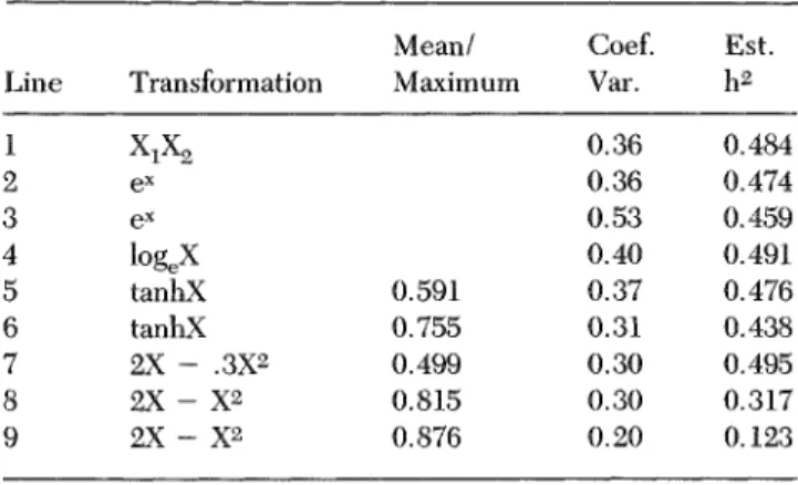
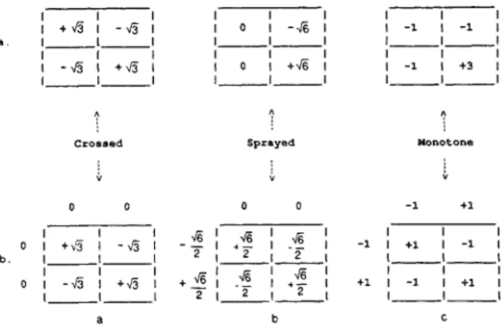
The simple multiplicative model is not the only reason-able alternative to additivity when different strains are Involved. If the response is linear for each strain, there is no reason why the Y Intercept should always be zero, as with Y = H#E. Consequently, several other models shown in Figure 2a were assessed for power of main effects and interaction. Certain of these were similar to models proposed for interacting genetic and cultural inheritance (Cavalll-Sforza & Feldman 1.973) and for mental disorders (Kendler & Eaves 1986). Because the "norm of reaction" Is often not linear when a wide range of environments is evaluated (Henry 1986), two nonlinear models were also considered. Although it is sometimes proposed that the norm of reaction is genetically deter-mined (e.g., Hull 1945; Schmalhausen 1949; Via & Lande 1985), this is not realistic because the response to a new environment also depends on prior rearing conditions (Denenberg 1977). Nevertheless, for clarity, each model assumes that any parameters (a, b) are specified by heredity and that parameter values are equally spaced for the five strains. Rather than derive the ratio of effect sizes (fH/fj) using algebra, a computer program was written to
generate expected means for a five strain by five environ-ment (X = value of E) design and then to calculate crH,
uE, and ar Table 4 presents power estimates for each
model when n = 10 and a = 0.05. The largest main effect, be it for H or E, is taken to have a large effect size, f = 0.4. In no case does the power of the test of interaction achieve an acceptable level of 80% or more when one or both main effects are virtually certain to be detected with ANOVA. It comes close to 80% for two Y = a + bX models, but when main effect size is 0.3 for these, the power of the test of main effects is 98% but the power of the test of H X E interaction is only 46%. The, power of the test of interaction is relatively low even when the directions of effects of environment are opposite for several strains (Y = a + bX, Case 1, and Y = aXe~b x), or when the rank orders of the strains change across environ-ments (Y = a + bX, Case 2).
a. EXPECTED VALUES FOR FIVE STRAINS
1 2 3 0 1 2 3 4 1 2 3 4 5
ENVIRONMENT (X)
b. PROFILES OF SIMPLE MAIN EFFECTS z o 2 ' O 4 DC 2 3 4 5 1 2 3 4 5 0 1 2 3 4 1 2 ENVIRONMENT (X)
Figure 2. (a) Expected values of a measure Y under six models for five strains of mice reared in five different environments where levels of environment (X) are 1.0 units apart. Parameters of each model are assumed to be determined by each strain's heredity, (b) Profiles of simple main effects of heredity at each level of environment for the six models in Figure 2a, expressed as a proportion of the combined sum of squares for heredity and heredity by environment interaction.
The inescapable conclusion is that the usual application of two-way ANOVA Is relatively insensitive to the pres-ence of real nonadditivity of the kind considered plausible by many investigators. There are basically two views about this reality. If the principal objective is to partition variance and calculate heritability coefficients, this may be seen as evidence that analysis of variance is "robust" with respect to the assumption of additivity. On the other hand, if the goal is to understand the nature of develop-ment, the way things work, there will tend to be skep-ticism about a statistical procedure which takes data that, to the educated eye, show obvious differences in slopes and shapes of the norm of reaction for different strains, and apparently crunches them into a set of parallel straight lines. From the latter perspective, it will be Table 4. Effect sizes and power for six models using J = K = 5, n = 10 and a = 0.05
Model Y = H + Y = H-E Y = a + Y = a + Y = a(l -Y = aXe' E bX, bX, - e - b x Case Case - b x ) 1 2 Effect fH 0.40 0.40 0.40 0.00 0.26 0.40 sizes fE 0.40 0.40 0.00 0.40 0.40 0.34 0.00 0.19 0.28 0.28 0.14 0.21 Power H >99 >99 >99 — 90 >99 of tests E >99 >99 — >99 >99 >99 of HxE 36 78 78 19 47
Wahlsten: Heredity-environment interaction difficult to understand how any inquiry could possibly
benefit from a test with inherently low power which often yields deceptively simple results.
It is noteworthy that techniques which estimate heritability by assuming n o H x E interaction can yield strongly biased estimates when certain kinds of interac-tion are indeed present in the data. After a detailed mathematical study of path analysis, Lathrope et al. (1984) concluded that among "the principal effects of interaction are a mean overestimate of the genetic heritability" (p. 618). One hopes that this finding will not discourage investigators from seeking better ways to detect H X E interaction and its consequences.
9o The perception of simple main effects
If ANOVA is so insensitive to interaction, then alternative approaches are required. Taking the relationships in Figure 2a, which usually yield nonsignificant H X E interaction terms, let us construct for each one a profile of expected simple main effects of heredity or strain dif-ference at each level of environment (Figure 2b). For each of these examples there are five levels of E and hence five simple main effects of heredity. The total of the sum of squares (SS) for these five must be equal to the SS for the main effect of heredity plus the SS for H X E interaction (Winer 1971). Thus, we can compute, at each level of E, the proportion of (SSH + SSHE) which is
accounted for by that particular simple main effect. If the relation between H and E is truly additive, then that proportion should be the same across all levels of E (Figure 2b). On the other hand, the profile of simple main effects is markedly uneven for the other cases in Figure 2b. An obvious departure of this profile from a horizontal line should alert us to the possible presence of nonad-ditivity in the relation between H and E, and thereby caution us against accepting a null hypothesis as true merely because we cannot conclusively prove it false. The need to interpret the pattern of results by careful inspec-tion is emphasized by Bolles (1988), whose Rule 5 is: "Always, always plot up the data to see what the numbers say. The numbers that you collect in an experiment will tell you if you have found something, even while statis-tical tests are fibbing, lying, and deceiving you" (p. 83). The utility of this approach is sometimes recognized implicitly when scientists look at graphs from a two-factor experiment, perceive what appears to be interaction, and then do separate t tests to confirm this impression. But does this approach truly prove the existence of nonad-ditivity? One example suggests caution. The most widely cited report of heredity-environment interaction in psy-chology is the Cooper and Zubek (1958) study of the McGill "bright" and "dull" rat strains (bred selectively for errors on the Hebb-Williams mazes) reared in three laboratory environments (restricted, normal, and en-hanced). (As Platt & Sanislow [1988] point out, the data for rats in the "normal" environment actually came from a separate experiment performed earlier.) The authors compared various pairs of the six groups, totalling only 65 rats or 10.8 per group, using separate t tests, and it is generally believed that this demonstrated H X E interac-tion (Platt & Sanislow 1988). However, an ANOVA on the six groups using raw data kindly provided by R. M. Cooper reveals significant main effects of strain (F = 4.98,
p < 0.05) and environment (F = 14.33, p < 0.01) but no significant interaction (F = 3.07, p > 0.05). The F ratio
for H X E interaction is slightly below the critical value of 3.15. Properly speaking, the data provide suggestive evidence but not conclusive proof of H X E interaction. The mere observation that two strains differ significantly at a = 0.05 In one environment but not in another does not necessarily warrant rejecting the hypothesis of ad-ditivity. After all, one value of t might be just great enough to achieve significance while the other t falls a bit short of significance. In the Cooper and Zubek (1958) data, the strain difference was obviously large in one environment and small in the others, which was quite sufficient to convince most of us that there was H X E interaction.
10. Sample sizes for detecting interaction
It would seem that many studies of heredity and environ-ment end up in a twilight zone of Inconclusive results where different people can easily Interpret subtle pat-terns in the data to be hints of this or that, where the fading hopes of some are kept alive by "almost significant" interaction effects or results "tending in the direction of significance," while others are relieved that the interac-tion effect was not quite large enough to rule out heritability calculations. From a statistical standpoint, the studies often lack sufficient power to shed much light on the nature of H X E interaction.
Looking closely at the data may help us avoid such serious mistakes as accepting a false null hypothesis, but the gaze of an experienced investigator is also fallible and can never be a complete substitute for a statistical test. Outright rejection of additivity really ought to require a significant interaction term in the ANOVA. If we are careful to avoid Type I errors when testing for the presence of main effects, surely we should also try to avoid them when testing for interactions. Why opt for a more complex model if it really isn't necessary?
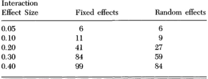
Perhaps we would be wise to anticipate these various difficulties and address them at the design phase before data are collected. If the effect size for a plausible kind of interaction is substantially less than for the main effects, then a larger sample size will be required to detect the Interaction than will be needed merely to detect average effects of the treatments. If it really matters whether or not the phenomena being studied are nonadditive, one needs to use larger samples than are customary for finding main effects. Proving nonadditivity false requires, at the very least, that the power of a test of interaction be substantial, 80% or preferably 90%, and that a proper sample size be chosen to guarantee sufficient power. Cohen (1977) provides convenient tables of sample sizes which yield different degrees of power for various effect sizes. A normal approximation that is useful when the interaction term has one degree of freedom is provided by Lachenbruch (1988). As shown above, for a two strain by two environment experiment the effect size for interac-tion under the Y = H-E model will be fj- = 0.133 when main effect sizes are large (0.40). The required sample sizes to detect such an Interaction at powers of 80% and 90% with a = 0.05 are more than 125 and 167 subjects per group, respectively, according to Cohen's tables. These values may appear extremely large, but the analysis of
Wahlsten: Heredity-environment interaction
variance with its definition of interaction as leftovers demands large samples. What reason could one possibly cite for using an analytical device because of its ability to detect nonadditivity, yet choosing a sample size that renders it ineffective? The finest optics in the world will portray a fuzzy image if the camera is out of focus or shaking.
informations
It is sometimes proposed that interaction in any kind of factorial design be addressed by transforming the scale of measurement to make the main effects additive. For example, Dunn and Clark (1974) recommend the pro-cedure of Tukey (1957) whereby a computer is used to find the values of the constants C and p in the transforma-tion (Y 4- C)p which minimize the size of the interaction term relative to main effects. In biometrical genetics in particular, the investigator is advised to search for a transformation that will eliminate heredity-environment interaction entirely, so that heritability and other param-eters can then be estimated (Jinks & Broadhurst 1974, p. 11; Mather & Jinks 1982, p. 64).
Is this approach legitimate? Perhaps it is, if there is no other way to meet the assumptions of equality of within-group variances, normality, and independence of errors. When a mean-variance correlation occurs for response time measures or when many observations in some groups occur near the upper or lower limit of the scale, a transformation may be necessary to permit a valid test of significance, and such a transformation may also elimi-nate a two-way Interaction. If the interaction does have a rather trivial origin in mean-variance correlation, then the transformation may be warranted. Even then, there may be pitfalls inherent in the procedure, because pa-rameter estimates of the logarithm of a variable, for example, can produce biased estimates of the un-transformed measure and can distort the estimates of variance components (Heth et aL, 1989; Kvalseth 1985). There has been some dispute in the pages of the
Psychological Bulletin about whether the scale of
mea-surement affects decisions about statistical significance, with arguments that it does not (Davison & Sharma 1988; Gaito 1980) and counterexamples showing that it can (Townsend & Ashby 1984), but this particular dispute has been focussed on comparisons of two independent groups. Concerning the consequences of transformation for two-way interaction, there Is no doubt that conclu-sions can be drastically altered. The question is: should they be altered?
The model on which ANOVA is based assumes equal-ity, normalequal-ity, and independence of within-group devia-tions, but It does not assume additivity of effects, al-though path analysis does (Wright 1921). Transformation solely to eliminate interaction Is a device to create the appearance of simplicity in the data, and there is a danger that this will be an entirely false appearance. For those who wish to learn how development actually works, wholesale and ad hoc testing of various transformations for the express purpose of getting rid of H X E interaction is counterproductive, because the shape of a functional relationship between variables provides a valuable clue to their causal connections. On the other hand, those whose only goal is to parcel out the variance among separate
causes can proceed only in the absence of H X E interac-tion and therefore they may be more willing to transform the scale of measurement, even if causal relations become distorted.
To return to the gravitation example, we can see that transformation of scale can radically alter the causal or explanatory model If we apply a logarithmic transforma-tion to Newton's law, the equatransforma-tion becomes additive.
In F = In - rl^m2 = ln-G + In 1 + In m2 - 2 In d Physicists use this approach to,analyze sources of mea-surement error, but they do so from a perspective very different from that of investigators who choose a transfor-mation without knowledge of the form of a genuine law of nature. If we let the log transformed variables in New-ton's law be the primed (f) variables, it reads: F; = Q? +
m^ -f m2' — 2 d\ The interpretation of this equation is
altogether different from the real law If we forget about the transformation and take the terms at face value. Addi-tivity implies a causal model which separates the contri-butions of the two masses, whereas the multiplicative
•F
d'
model Implies mutual interdependence. Newton achieved a profound insight, which had eluded most predecessors who regarded the weight of an object as an inherent property of that object itself, something that existed in isolation from its surroundings. He argued that every speck of matter in the universe has mutual attrac-tion with every other speck. Mutual attracattrac-tion is ex-pressed as the product of the masses. The weight of an object Is the result of its Interaction with other objects. It makes no sense to say that a person's weight depends more on body size than planet of residence. The additive model is really no simpler than the multiplicative one, in that both have three variables and a constant. The log transform alters the relations among the variables; conse-quently, transforming the scale of measurement may conceal the relations among heredity and environment, as it might conceal the essence of gravitation.
Transformation to suppress H X E interaction may create further obstacles to applying the knowledge gained from ANOVA. Consider the first use of ANOVA for a two-way factorial design by Fisher and Mackenzie (1923) to examine the yield of 12 potato varieties under six condi-tions of manure at the Rothamsted Experimental Station. Yields ranged from 26.5 lbs. per row for the Up to Date variety with farmyard dung to 1.6 lbs. per row for the hapless "undunged" Duke of York. The effect of sulfate of potash appeared to depend strongly on variety of plant and presence of dung, but the interaction term was not significant, although main effects were large. Inspecting their data, Fisher and Mackenzie observed a nonadditive pattern whereby higher yielding plants benefitted more from manure; they accordingly wrote that: "A far more natural assumption is that the yield should be the product of two factors, one depending on the variety and the other on the manure" (pp. 316-17). Rather than transforming their original observations of yields, they showed that the data "are better fitted by a product formula than by a sum
formula" (p. 320). Modern quantitative behavioral genet-ics, however, would dictate a transformation to achieve additivity. Such a procedure may be convenient for the theorist, but the everyday men of the soil must sell their potatoes by the pound and purchase manure by the ton. If there is a variety whose yield increases more than others for the same bulk of fertilizer applied, they would cer-tainly want to know about this. After all, they cannot pay their bills in the square root of pounds sterling. To the farmer or scientist struggling to understand how things grow or develop, real interactions should not be hidden by ad hoc scale transformations.
Of course, transformation of scale need not conceal information. If we can discover a transformation that effectively eliminates interaction from the ANOVA, this reveals something about the mathematical structure of the original observations (Lubin 1961). There is no se-rious harm in generating additivity with a logarithm, provided the investigator remembers to calculate and report the anti-log when interpreting the results, rather than reifying the additivity. For example, Box and Cox (1964) used a log transform of a measure of strength of worsted yarn in a three-way ANOVA to demonstrate that the relations among weight of the load, length of yarn, and duration of loading are multiplicative because the log of strength eliminates the interactions. A problem arises when the original data are transformed and the profound effects of the change of scale on the causal model are neglected when presenting the results. If H and E really are multiplicative in a particular situation, a calculated "heritability'5 is nonsensical and taking the log of the observations may compound this.
The primary remedy proposed here for the problem of the low power of tests of interaction is the same as the one suggested by Neyman in 1935: Use larger samples, sup-plemented by a large dose of caution and rigor when interpreting results. Are other, possibly more palatable solutions available?
Neyman (cited by Traxler 1976) also proposed that additivity should be affirmed only if the main effects are significant at the 0.01 level, whereas interactions are not significant at the 0.05 level. Using different a levels could indeed reduce or even eliminate the imbalance in the power of the tests, although this could become rather cumbersome because the values of a required to equate the powers would depend on the specific alternative model being contrasted with the additive model. Fur-thermore, if the a level is set at 0.05 for the interaction term, the larger samples documented in section 10 are still required.
The interaction term in a J X K factorial design pro-vides a global test of all possible kinds of deviations from strict additivity and hence may not be very sensitive to particular kinds of nonadditivity. It is possible to test more specifically for linear interactions whereby groups at different levels of one factor have different slopes of linear response to levels of the other factor or when the factors are thought to be multiplicative (Freeman 1973; Mandel 1961). Perkins and Jinks (1973) used a similar approach to show that large variations among 82 strains of tobacco plants in response to 16 fertilizers were almost
Wahlsten: Heredity-environment interaction entirely due to interactions of the linear type. These procedures will probably have greater power than the global F test, although the amount of gain has not been evaluated. However, there is concern that these tests may be biased (Roux 1984). Of course, they can provide no improvement at all for a 2 X 2 design and are need-lessly complex for modest experiments having few de-grees of freedom for the interaction term, which can be assessed more readily with orthogonal contrasts (Lachen-bruch 1988).
A more radical departure from the standard ANOVA procedure is provided by the likelihood ratio test (Marler 1980), which compares the likelihoods of a particular set of data according to two distinct hypotheses, neither of which must serve by default as the null hypothesis. This approach can be extended to more than two reasonable alternatives, as done by Debray et al. (1979). Similarly, one could compare additive and various nonadditive models of heredity and environment in a factorial design. These calculations require much more effort from the investigator and considerable computing time, but they should yield greater statistical power than the ANOVA approach. Unfortunately, this would also require much greater mathematical knowledge on the part of the reader.
13. Heritability and eugenics
Analysis of variance may be useful in identifying signifi-cant sources of individual differences, but its insensitivity to the underlying mathematical structure of functional relationships limits its utility to the early phases of inves-tigation. If variations in both heredity and environment are found to contribute to individual differences in behav-ior, then the next phase of the research ought to look more closely at the intricacies of the two processes in the developing organism using larger samples and more sen-sitive analytical methods. Simply to cite a heritability coefficient or compare the relative strengths of the main effects of heredity and environment in a factorial experi-ment does not advance our understanding of the nature of development.
Unfortunately, estimating heritability seems to be the main, objective of some investigators. As Kevles (1985) and Fancher (1985) have documented, many of the found-ers of human behavioral genetics were committed to a program of eugenics. The only practical application of a heritability coefficient is to predict the results of a pro-gram of selective breeding. The rate of change in the average value of a characteristic during the first few generations under a regime of artificial selection of breeders will be directly proportional to the heritability (in the narrow sense) of the characteristic in the popula-tion. If such a goal is eschewed, there is no compelling reason to focus attention on "heritability" and ignore interaction.
14. Gene action Is interactiwe and dynamic Of course, statistical problems are not the only challenges to theories of additivity of heredity and environment, and statistical solutions are not likely to settle this dispute. Perhaps the greatest weakness in the Y = H + E model is the assertion that the effects of one's heredity on
develop-Wahlsten: Heredity-environment interaction
ment are entirely separate from those of one's environ-ment. This claim is contradicted by many discoveries in developmental biology.
There are now good reasons to believe that the genes in the nucleus do not contain a program for development or a blueprint for brain structure (Gerhart 1982; Stent 1981). The timing and spatial location of important events in development are not directly specified by information intrinsic to the genes in the nucleus (Davidson 1987; Easter et al. 1985; Oyama 1985). Rather, a gene codes or programs for a protein or enzyme, and the consequences of this activity at the level of macromolecules for events at the cellular and organismic levels, depend on other parts of the cell, other cells in the growing organism, and even events outside the organism. The metabolic activities of DNA molecules are subject to control by factors outside the nucleus of the cell (Blau et al. 1985). The actions of certain genes can be modified greatly, even sometimes switched on or off entirely, by changes In temperature (Atkinson & Walden 1985; Helkklla et al. 1986), light (Klein & Yuwiler 1973), diet (Benkel & Hickey 1987), and even the maternal environment (Carroll et al. 1986). Developmental biology is tuned in to nonadditive pro-cesses (Pritchard 1986). Direct evidence of biochemical gene action in an environmental context supports a dyna-mic and interactive view.
The continued use of statistical tests insensitive to interaction is distressing, not merely because it fosters a false impression that heritability analysis is justified, but because valuable information about processes of develop-ment may be lost. A knowledge of interaction deepens our understanding of how living things acquire form and motion. According to Lubin (1961): "The most important questions that can arise from a statistical finding of in-teraction are those which are non-statistical. . . . For me, significant interactions raise two most Important ques-tions: How does this Interaction occur? How can I bring it under experimental control?" (p. 816). Likewise, for Lassalle (1986), H X E interactions should be viewed "as powerful tools which can assist us in understanding the underlying processes of behaviour" (p. 205), and for Bateson (1987) "analyses of statistical interaction should be the starting points of attempts to understand how developmental processes work and should not be treated as ends in themselves" (p. 2).
ACKNOWLEDGMENTS
Supported in part by grant 4878 from the Natural Sciences and Engineering Research Council of Canada. I thank Margot And-ison for drawing Figure 1 and Susan van Ballegooie for typing the manuscript. The initial version of this paper was written when the author was at the Department of Psychology, Univer-sity of Waterloo, Ontario.
NOTES
1, Effect size f for a one-way AN OVA is related to an alter-native measure of effect size, the proportion of total variance attributable to differences among group means, termed T|2 by Cohen (1977) and w2 by Hays (1988), according to the relation
parameter of the noncentral F distribution, X, or related mea-sures 8 or <|), with the following relations among them for J groups of n observations each:
8 X 2. Principal steps in = fVn = d>Vj == f VnJ , = 82 = f%J.
the derivation of CJE are
kQ + 2 )(K + l)he 4 l)he M, (Mt -__ (J + l)2(he)2K(K -k = l
For finding ap the first step for each group is:
Across all J°K groups, this yields:
2 i (Mjk-MrMk+M)2 = JKa+l)a-l)(K+l)(K-l)(he)2 j=lk=l
3o The tables in Cohen (1977) and most other sources on power of AN OVA apply directly to a one-way design, but our interest here is in a two-way factorial design. Cohen (1977) addresses this problem by noting that a mean for one level of the first factor across all levels of the other is not based on only n observations; rather, it is based on nK observations. Of course, a few degrees of freedom are lost because of constraints placed on the data in computing between-groups sums of squares; hence, the effective sample size (n?) for a test of the main effect of heredity is
Af
+ 1 = K(n - 1) + 1.
^between +
When there are 5 strains reared in 5 environments and n = 10 subjects per group, effective sample size per strain for the test of the main effect is 46. For the test of interaction, n' = 14.2 because
+ 1 = JK(n - 1)
(J - 1)(K - 1) + 1+ 1.
That is, the power of the test of the interaction term is essentially the same as the power of a test of variation among 17 groups with 14.2 observations per group in a one-way design.
Rather than deriving all values of power by interpolation from the tables given by Cohen (1977), the normal approximation to the noncentral F distribution (Severo & Zelen 1960) was used. This is not the best available approximation (Tiku 1966), but it is reasonably good when we are interested in statistical power to only two decimal places or the nearest percent, and it is much easier to compute.
1 +
For co2, small, medium, and large effect sizes would be about 0.01, 0.06, and 0.14, respectively. Cohen (1977) gives power in terms of f, but several other sources use the noncentrality
Commentary/Wdihlsten: Heredity-environment interaction
Commentary submitted by the qualified professional readership of this journal will be considered for publication in a later issue as Continuing
Commentary on this article. Integrative overviews and syntheses are especially encouraged.
lurement
Fred L. Bookstein
Center for Human Growth, Department of Biology, University of Michigan, Ann Arbor, Mi 48109-0406
Electronic mail: [email protected]
Wahlsten's target article inquires about when it "makes sense to attribute a definite percentage of variation in some measure of behavior to variation in heredity." Yet the discussion does not touch upon technical aspects of heritability per se, such as the relations between parental and offspring scores. Instead, the fallacies of the behavioral genetics literature surveyed here exemplify confusions about the meaning of quantification in science that run far deeper.
To ask, with the target article, "Y = H + E - true or false?" is to conceal the underlying issues of mensuration. The scientist and the user of analysis of variance (ANOVA) approach the issue of describing Y, H, and £ radically differently. Whereas the scientist would demand that E and H be measured in their own units, the user of ANOVA implicitly "measures" categories of £ and H using the units of Y instead. When main effects are measured in units of the dependent variable, then the H X E interaction has no operational meaning as an amount of anything "per" anything else; it has no units; it is not a measurement. The relevant aspect of Newton's law of gravitation, reviewed in the target article, is that masses are measured in units of mass, not in units of force. It is this possibility of direct measurement, regardless of functional form, that saves the physicist from the futilities of ANOVA.
Once H and £ are measured directly, the issue of "interac-tion" is trivial. Temporarily, in the interest of clarity, assume that we already know how to measure H and £ as numerical variables x and z, and that the true law describing the depen-dence of Y on x and z is some noise-free function Y = f(x,z). In this setting, the condition equivalent to absence of the interac-tion term in an ANOVA of Y upon H and £ is that / be "separable":
f(x,z) = g(x) + h(z), (la)
the mathematical functions g and h replacing the familiar "main effects" of H and E. The assertion of separability is a single partial differential equation of second order:
dxdz = 0 everywhere. Ob)
But no particular interest inheres in this separability condi-tion in the absence of other equacondi-tions governing the behavior of g and h. (For instance, in classic studies of intergenerational heredity, g takes the form of a linear regression to the mean.) When such additional equations are not forthcoming, the knowledge of separability (absence of interaction) is of no partic-ular value, as it can always be guaranteed by small changes in the measurement system. Define a critical point of/as an (x,z) pair where both first-order partial derivatives
hf/bx and hf/hz
are zero at the same time. It is a theorem that any/(x,z) without critical points in a region of interest can be expressed as perfectly linear in some deformed version of the (x,z) - coordinate system. The theorem, a prologue to the so-called "Morse Lemma" (Poston & Stewart 1978, sec. 4.2), guarantees that we can write
(2)
(no further terms), where x; = x + small stuff and z' = z + small stuff are gently nonlinear functions of the originally measured x and z. For an exploration of this and other aspects of catastrophe theory, refer to Poston and Stewart.
Thus, in the absence of critical points we can always make an interaction term disappear by slightly altering our scheme for measuring x and z. The presence of critical points is far more important than this: It is generic, not an accident of small changes in measurement systems. Consider (Figure 1) the two surfaces y = - x2 - z2 (left) and y = x2 -z2 (right). Neither has any "interaction terms" like xz - but they could not be more different in their scientific implications. Whereas the former has a global maximum at one point (0,0) of the domain of its arguments, the latter goes off to ± °° twice each as one goes around lines through the origin. (The cases are distinguished by the sign of the discriminant B2 — AC of the quadratic
approx-imation Ax2 + 2Bxz + Cz2 to Y.) Rewriting x2 - z2 as (x + z)(x
-z), we see again that, as the target article avers, there is no
intrinsic difference between additive ("interaction-free") and multiplicative models. Instead, there remain huge differences among varieties of critical points even in the absence of
interac-tions. The presence of a "statistically significant" interaction
term - say, 2xz - doesn't tell us whether the situation is free of critical points or, if not, whether it resembles more the ex-tremum, the saddle surface, or some other more exotic possibility.
In a stochastic setting (noise present),. the separability condi-tion (la) or (Ih) is replaced by a statement about expected values: for any z} and z2, we are asserting that E\f[x,z^) ~f(x,z2)]
is independent of x (from which it follows that E\f[xvz) -/(x2,z) ]
must be independent of z). In most applications, E\f(°,z)] will then exist as an expectation, for fixed z, over the universe of possible x's as they substitute for the dot under stratified sam-pling, and likewise £[f(x,°)] exists as an expectation for fixed x over stratified sampling of zs. But, as we have seen, it is not the existence of these expectations that is the scientific issue here -we can almost always redefine x and z jointly so that these expectations exist and can be computed either via formula (2) or by sums of squares analogous to those in Figure 1. It is the forms of the functions E\f[-,z)] and £[f(x, •)] that are crucial, specifical-ly, the number and genres of their critical points, regardless of any interactions.
Analysis of Y, H, and E culminates in scientific understanding of the determination of Y only when the factors H and E have been explicitly measured separately and independently. The mensural fallacy underlying the literature criticized in the target article arises in the confusion between the H and £ of "Y = H +
E" - continuous variables x and z — and if and E as the mere names of "groups" or "strains" or "conditions" not otherwise
calibrated. In the absence of interaction, the ANOVA computes £[Y|if = h] and declares it to be the "value" of each state h of H,
Figure 1. (Bookstein). Two mathematical surfaces, each free of interaction terms, which show essentially different behavior in the vicinity of their critical point, (left) y = — x2 — z2. (right) y =