HAL Id: inria-00071646
https://hal.inria.fr/inria-00071646
Submitted on 23 May 2006
HAL is a multi-disciplinary open access
archive for the deposit and dissemination of
sci-entific research documents, whether they are
pub-lished or not. The documents may come from
teaching and research institutions in France or
abroad, or from public or private research centers.
L’archive ouverte pluridisciplinaire HAL, est
destinée au dépôt et à la diffusion de documents
scientifiques de niveau recherche, publiés ou non,
émanant des établissements d’enseignement et de
recherche français ou étrangers, des laboratoires
publics ou privés.
Global visualization of experiments in ad hoc networks
Dominique Dhoutaut, Quang Vo, Isabelle Guérin Lassous
To cite this version:
Dominique Dhoutaut, Quang Vo, Isabelle Guérin Lassous. Global visualization of experiments in ad
hoc networks. RR-4933, INRIA. 2003. �inria-00071646�
ISSN 0249-6399
a p p o r t
d e r e c h e r c h e
TH `EME 1
INSTITUT NATIONAL DE RECHERCHE EN INFORMATIQUE ET EN AUTOMATIQUE
Global visualization of experiments in ad hoc
networks
Dominique Dhoutaut, Quang Vo, Isabelle Gu´erin Lassous
No 4933
Unit´e de recherche INRIA Rhˆone-Alpes
655, avenue de l’Europe, 38330 Montbonnot-St-Martin (France)
T´el´ephone : +33 4 76 61 52 00 — T´el´ecopie +33 4 76 61 52 52
Global visualization of experiments in ad hoc networks
Dominique Dhoutaut, Quang Vo, Isabelle Gu´
erin Lassous
Th`eme 1 — R´eseaux et syst`emes Projet ARES
Rapport de recherche no 4933 — Septembre 2003 — 14 pages
Abstract: The real experiments in ad hoc networks study metrics that can be obtained with local monitoring on the machines. No global and full visualization of the experiments is proposed. However such a visualization can be very useful and can help in a sharp evaluation of the tested protocols. Setting this type of visualization requires a synchronization of the events performed during the experiment. In this paper, we propose a synchronization method that enables the setting up of a global visualization of experiments in ad hoc networks. Key-words: experimentations, ad hoc networks, visualization, synchronization
Une visualisation compl`
ete des exp´
erimentations dans
les r´
eseaux ad hoc
R´esum´e : Les exp´erimentations r´eelles dans les r´eseaux ad hoc s’int´eressent `a diff´erentes m´etriques qui peuvent ˆetre obtenues grˆace aux traces locales pr´esentes sur les machines `
a l’issue des exp´erimentations. Aucune visualisation compl`ete et globale n’est utilis´ee sur les exp´eriences actuelles. N´eanmoins, une telle visualisation peut ˆetre tr`es utile et tr`es b´en´efique pour une compr´ehension en profondeur des protocoles test´es. Mettre en place ce type de visualisation demande une synchronisation des ´ev´enements qui se sont d´eroul´es lors de l’exp´erimentation.
Dans cet article, nous proposons une m´ethode de synchronisation pratique qui permet de mettre en place une visualisation globale des exp´erimentations dans les r´eseaux ad hoc. Mots-cl´es : exp´erimentations, r´eseaux ad hoc, visualisation, synchronisation
3
1
Introduction and objectives
An ad hoc network is a wireless and mobile network without any fixed infrastructure. When a mobile transmits data, they are received by all the mobiles within the communication range of the emitter. To enable the communication between any pair of mobiles, a routing protocol is needed. Researches in ad hoc networks have essentially been devoted to the design of routing protocols. The evaluation of such protocols is often carried out by simulations. Few experimentations on real ad hoc networks are realized to test and evaluate the proposed protocols. Different explanations can be given to this lack of experimentations in such networks:
• The difficulty to manage real experimentations: how to identify or set the topology of the network, i.e. the radio links (for instance how to position two mobiles that will communicate within two radio hops), how to deal with the instability of the radio links that prevents from the reproduction of identical experiments, the need of labour in case of large and mobile networks, etc.
• Few softwares have been implemented with the goal to ease the experiments and the tests of protocols in real networks.
• The lack of solutions to handle the logs of the machines implied in the experiments in order to evaluate and to monitor their run.
To our knowledge, few works deal with such experiments. The works of [8, 9, 13] aim at depicting the behaviour of some particular routing (DSR for [8, 9] and ABR for [13]). Only APE [6] and Forwarding [2] are completely dedicated to experiments. Their goal is to ease the deployment of scenarios on real ad hoc network. APE concerns essentially the evaluation of routing protocols whereas the aim of Forwarding is to test the MAC protocols. As mentioned in [7], the studied metrics during experiments are essentially packet loss, jitter, end-to-end delay, throughput. All these metrics can be obtained with local log files collected during the experiment. No global visualization of the the run of the experiments is provided in the previously mentionned works. But it can be very useful to get a global log of the experiments. Such kinds of logs can give information on the schedule of the packets during the experiments, the possible spatial re-use, the possible collisions, etc. Such informations help in a better understanding of the protocols under evaluation.
The global visualization of an experiment may be done with the fusion of the local log files of the machines and the synchronization of the events extracted from these local log files. A unique time scale, corresponding to the time of the experimentation, enables such a global visualization of the experiments, i.e. to know at any given time which mobiles send which packets to which other mobiles and to have a full knowledge of the run of the experiments.
Many protocols have been designed for synchronizing the physical clocks of computers in network. Most of the protocols concern wired networks and the synchronization in ad hoc networks seems to be much more complicated. The synchronization problem has become
4
very popular with the use of sensor networks [1]. Wireless sensor networks, composed of small-scale wireless nodes, cooperate in order to fulfill monitoring complex tasks. But as claim by the authors of [5], none of the synchronization solutions proposed for sensor or ad hoc networks can be considered the best: they are often cost-effective in terms of messages exchange or they do not provide an accurate precision. Moreover, these authors recommend a post-facto synchronization without the need to keep a global timescale on each node at any time.
Building global logs of an experiment does not require a time synchronization at runtime, it can be provided with a a posteriori synchronization of the local logs of each machine implied in the experiment. Indeed, the mobiles do not need to be synchronized and can run with their local time during the experimentation if the local times can be translated, after the experiment, to a consistent global time that corresponds to the real time of the experiment.
In this paper we present a method to realize a global visualization of real experiments in ad hoc networks with the use of a a posteriori synchronization. In Section 2, we describe the different time synchronization protocols designed for ad hoc and sensor networks. In Section 3, we describe the proposed solution. We test our solution on an ad hoc network composed of a five nodes chain and present a possible visualization derived from the a posteriori synchronization.
2
Time synchronization protocols for ad hoc and sensor
networks
Clocks synchronization is a basic problem that arises in various fields, like networks, but also distributed systems or real time systems. The goal is to keep the different clocks of the system as close as possible. The accuracy comes from the used algorithms, but also from the topology of the system, the communication links, the load of the machines, etc.
Many solutions exist, especially for traditional systems. NTP [10] is the famous synchro-nization system used in the Internet. Based on a tree structure of servers, the synchroniza-tion is done layer by layer. If this system is very efficient in the Internet, it does not seem adapted to multihop wireless networks. As mentioned in [5], the assumptions made by NTP are not true in wireless sensor networks: for instance, it uses much energy and it is based on an infrastructure with a relatively stable topology. Specific techniques are needed for such multihop networks.
The field of wireless sensor networks is very interested in time synchronization. More synchronization protocols have been proposed for sensor networks than for ad hoc networks. This can be explained by the goal and the use of these networks: many monitoring appli-cations are developped in sensor networks that required data fusion often subject to time synchronization.
The protocol RBS (Reference-Broadcast Synchronization), described in [4], can achieve a 1µs precision in a one-hop area (all the mobiles are within a broadcast domain). Its
5
extension to multihop networks leads to a degraded accurarcy (still of the order of the µs). In the multihop context, RBS needs to maintain a routing structure between the broadcast zones. In [11], the authors propose to set and maintain a cluster of the broadcast zones taking into account the synchronization accuracy, the power efficiency and the robustness. A post-facto synchronization is proposed in [3]: the synchronization is done just after the communication. It avoids to consume energy for time synchronization at all times and enables the use of low-power mode as designed in some sensor networks.
As far as we know, [12] is the only paper dealing with time synchronization in ad hoc networks. The goal of this work is not to synchronize the clocks but to timestamp the packets using local clocks. The idea is to translate the local time of the source machine in the local time of the receiver after the packet transmission. Such transformations are not accurate enough and require the use of time intervals for the exact times. It achieves a 1ms precision. However, this accuracy depends on the transmission delay and the number of hops between the source and the receiver.
3
A global visualization
A mentionned in Introduction, all the results reported by experiments in ad hoc networks ([8, 9, 13, 6, 7, 2]) concern local results on the packets (end-to-end delay, jitter, lost packets, etc.), on flows (throughput) and on each mobile (number of packets sent or forwarded, etc.). No global results, corresponding to the run of the experiment, are given. Such global results could give, at any time of the experiment, which mobile sends which packet to which other mobile, which mobile receives which packet from which mobile, etc. Such informations enable to know what precisely happens during experiments and can strongly help in the understanding of the used protocols.
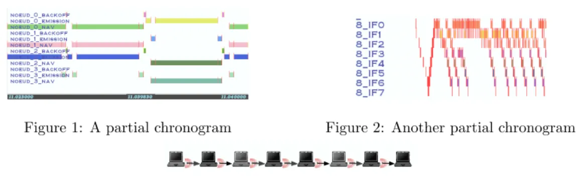
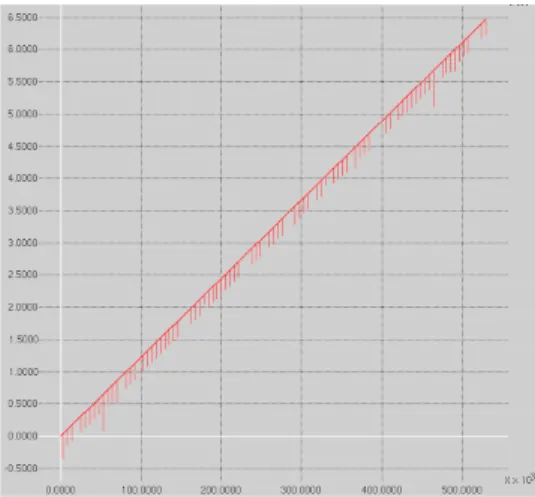
Henceforth, we call chronogram a graphic that gives the values obtained by some parame-ters of the experiment according to the time of the experiment. For instance, the chronogram given in Figure 1 represents different parameters of four mobiles during an experiment: the time is given at the bottom of the figure (this chronogram gives some information for the pe-riod between 11.023s and 11.040s of the experiment); the studied parameters correspond to the different states of the MAC layer that a mobile may have with the IEEE 802.11 standard. We are not going to detail 802.11, but for instance, this chronogram shows when a node emits (NOEUD 1 EMISSION), when its backoff is decreased (NOEUD 1 BACKOFF) or when it considers the medium busy according to its network allocation vector (NOEUD 1 NAV).
Figure 2 shows a chronogram obtained in a 8 nodes chain (Figure 3). Each node can only communicate with its directs neighbors, and the first node tries to send data packets to the last. The routing protocol is AODV. This time, only transmissions are presented. On this chronogram we can clearly see the RouteRequest and RouteReply exchange (the V shape at the beginning) used to construct the route, and then the data packets (which may be lost, usually at the second or third node).
Those chronograms are the result of two simulations under NS2. Simulators, like NS2, have a global clock common to all the simulated mobiles. With some time and some
6
Figure 1: A partial chronogram Figure 2: Another partial chronogram
Figure 3: A 8-nodes chain
ming, it is not difficult to obtain such chronograms. Within the context of experimentations, there is no common global clock in the ad hoc network and the different mobiles are not synchronized.
As mentioned in Section 2, some protocols have been designed for multihop networks. Some protocols for synchronizing sensor networks, like RBS, have an accurate precision. But these protocols need to maintain some informations at any time in the network. For instance, RBS maintains a routing structure of the broadcast zones. This permanent maintenance, as the permanent synchronization, may have an impact on the experiment. If the goal of the experimentation is to evaluate and to measure the performances of a protocol, the packets exchanged for the synchronization will be taken into account in the performance. And this can alter the evaluation, if accurate evaluation is required. Moreover, these protocols are not straightforward to implement on real networks.
As mentioned in Introduction, continous synchronization is not necessary for the global visualization. In [3], the authors propose a post-facto synchronization. As soon as a node communicates, a “third party” sends a synchronization packet just after the communication in the area of the communication. If the synchronization is not permanent, it implies a synchronization after each communication. This can also have an appreciable impact on the performances of the tested protocols. Therefore, we have opted for an a posteriori synchronization where the events are synchronized after the experiments.
3.1
A posteriori synchronization
The clocks of the computers are imperfect and subject to clock drift. According to [12], the clock drift on today’s computers is of the order of one second in ten days. We have made some experiments in order to evaluate a rough estimate of the clock drift of our available computers. Figure 4 shows the configuration of our experiment: the emitter broadcasts packets on the radio medium (with a wireless card implementing the IEEE 802.11 standard) that are received by two different receivers. Ten broadcasted packets of 1000 bytes are transmitted per second. When a packet is received, each receiver stamps it with its local
7
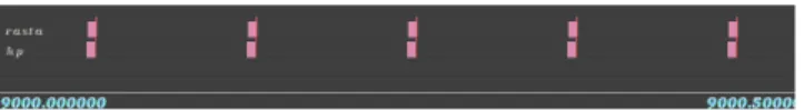
time. The experiment lasted for 14 hours and 30 minutes. To observe the clock drift, we consider the difference between the local times of each received packet on the two machines. Figure 5 shows this difference: without clock drift, each packet should be received at the same time whereas the results show that the difference between the local times of the two machines is of 6.5 seconds after 14h30. The machines have been synchronized at the beginning of the experiment, what explains there is no time difference for the first packet. If the difference seems rather linear, localized gaps may be noticed. As explained in [3] and [4], this is due to the variable delays on the receivers, caused, for instance, by nondeterminism in the detection hardware and operating system operations. Such delays are scarce since they only concern 1% of the total received packets during the experiment. As they do not occur consecutively and are easy to detect, it is possible to eliminate those packets. In the following of our work, we assume they have been eliminated and we do not take them into account anymore (we used a simple filter that detects variations too far from the average).
A delay of 6.5 seconds within 14h30 corresponds to a delay of 7.5 ms within one minute. Other measurements with the same experiment have been carried out on recent machines. The observed clock drift is around 0.3ms within one minute. This result is better but larger than the value given in [12]. Figure 6 shows a chronogam associated to this experiment: we see when each machine receives a packet broadcasted by the emitter. In the experiment each packet is received at the same time whereas the chronogram shows a notable delay between the receipts. This chronogram does not correctly describe the experiment. The transmission time of a 1000 bytes packet at 2Mb/s with 802.11 is around 4ms, whereas it is around 1.6ms at 11Mb/s. Therefore the measured clock drift can not be ignored for the setting of chronograms in the context of ad hoc networks. Otherwise the chronogram will not give the exact run of the experiment and no useful information will be able to be extracted. .
Figure 4: Experiment to evaluate the clock drift
A first approximation If we consider that the clock drift between two machines may be approximated by a straight line, then we can choose one machine as the absolute reference and correct the clocks of the other machines of the experiment thanks to linear coefficients. Each coefficient associated to each machine is computed from an experiment as described in Figure 4 where one receiver is the reference machine and the other receiver is the considered machine.
8
Figure 5: A clock drift (y-axis: difference of the local times) during 14h30 (x-axis: packet number)
Figure 6: A chronogram from the experiment of Figure 4
We have applied this method to our first experiment. We have choosen one receiver as the reference and we correct the clock drift of the other receiver thanks to the slope line computed from Figure 5 (the localized gaps have been eliminated and the slop is computed with the first point and the last point of the curve). We compare, after correction, the local times of each received packet on the two machines. Figure 7 shows that an error of synchronization still remains: the x-axis gives the error in ms (i.e. the difference between the local times after correction) and the y-axis gives the number of packets associated to each error. 520000 packets have been studied. Although the difference in synchronization is reduced, it remains still notable: many packets are received with a difference in time greater than 2ms, the maximum error being of 3.5ms and the mean error of 2.4ms. The approximation done in this method is not accurate enough for the setting of the chronograms in ad hoc context.
A second approximation We now cut the curve of Figure 5 in different segments, ap-proximate each segment by a straight line and apply the first method on each segment: one machine is used as reference, we compute the linear coefficients of each machine on each segment and we correct the received times with these coefficients. The accuracy of the
9
Figure 7: Distribution of the error with the first approximation (x-axis: error in ms; y-axis: number of packets with this error)
Segment length Maximum error Mean error
5 mn 0.23 ms 0.38 µs
20 mn 0.31 ms 4.4 µs
30 mn 0.44 ms 10 µs
60 mn 0.62 ms 30 µs
Table 1: Accuracy of the approximation with different segment lengths
synchronization depends on the length of the segments. If we apply this second method to the results observed in Figure 5 according to different segment lengths, we obtain different errors (maximum and mean errors), presented in Table 1. Figure 8 gives the distribution of the error with a segment length of 20 minutes (the x-axis and y-axis are the same as for Figure 7 and 520000 packets have been studied). We see that 95.6% of the total packets have an error smaller than 0.054ms and there are very few large errors. This means that if we are able to synchronize the network every 20 minutes, then we can use this method, i.e. approximate the clock drift of the machines according to a reference machine by a straight line and then correct the clock drift, to develop the chronograms.
From a practical point of view, the different log files, established during the experiment, can be synchronized with the following method:
10
Figure 8: Distribution of the error with the second approximation (x-axis: error in ms; y-axis: number of packets with this error)
• Synchronize all the machines at the beginning of the experiment with a transmitter that broadcasts synchronizing packets (all the machines need to be within the com-munication range of the transmitter).
• Run the experiment (no necessary condition, the machines may move, the network may be partitionned, etc.).
• Every 20 minutes, stop the experiment, group the machines within the communica-tion range of the synchronizing machine and synchronize them with the broadcasted synchronizing packets.
• At the end of the experiment, group the log files and use the describe method to synchronize the events according to the reference.
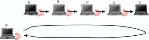
Figure 9 shows a chronogam associated to the experiment of Figure 4 with the use of this method. We see that, compared to Figure 6, the synchronization in the receipt of the broadcasted packets is much better, the chronogram correctly describes the experiment and the data given by this chronogram are usable.
A more practical method With the second method, all the mobiles need to be grouped in the communication range of the synchronizing machine at some time of the experiment. But to periodically move all the machines is not quite easy, especially when the experiment implies a large ad hoc network with many mobiles. It may require some time, labour and battery. Moreover, putting back the mobiles after the synchronization may create a different
11
Figure 9: Distribution of the error with an approximation by a line of 20ms segments (x-axis: error in ms; y-axis: number of packets with this error)
radio environment than the one experimented just before the synchronization and may have a notable impact on the results of the experiment. Rather than to group the machine during a synchronization period, we can move the synchronizing mobile towards the machines. The main difference with the previous method is that, under some topologies (multihop ones), the synchronizing mobile may not transmit its broadcasted packets to all the mobiles of the experiment at the same time. Therefore, it is no longer possible to compare the local times of the receipt of a same packet with the one of the reference machine of the experiment to compute the different clock drifts.
Then we have chosen to use as the reference machine the synchronizing mobile, i.e. the machine emitting broadcasted packets. Every 20 minutes, this machine moves towards the network in order to synchronize all the machines. With the knowledge of the transmision frequency of the broadcasted packets and with a packet number, each machine can compute the times of the receipts of the broadcasted packets within the reference clock, i.e. to know the time spent since the beginning of the experiment within the global time scale. It means that each mobile is synchronized with the reference machine every 20 minutes and that we can use the second approximation of the clock drift between two consecutive synchronization packets received by the machine. At the end of the experiment, we can correct the date of each event with the coefficients computed by the second method. Formaly, assume that synchronization packets are sent every k seconds then the receipt time (within the reference clock) of a synchronizing packet of number n is Tn = k × n. Assume that, for a machine,
ts1 and ts2are the local times of the receipt of two consecutive synchronizing packets with
respective numbers n1 and n2. The ratio between the global time and the local time spent
between the receipts of these two packets is R = k×(n2−n1)
ts2−ts1 . If a packet is received during
the experiment at the local time t, between ts1 and ts2, then the receipt time within the
reference clock is T = R × (t − ts1) + k × n1. We are thus able to translate the local times
of all the events of the experiment in the global time.
This method enables to synchronize the events a posteriori and to have a global view of the experiment.
3.2
A five nodes chain experiment
To test the faisability and the accuracy of our approach, we have carried out an experiment on a real ad hoc network. Figure 10 shows the topology of the tested network: the mobile Asends 1000 bytes packets to the mobile E at 2Mb/s (the mobiles use wireless cards
12
✁ ✂ ✄ ☎
✆
Figure 10: An experiment on a five nodes chain and the synchronizing mobile
menting 802.11). The packets are broadcasted. We have used the Forwarding software [2]: no routing protocol is used since the routing rules are set statically. The goal of Forwarding is to study the MAC protocols in the ad hoc context without the overhead of the protocols of higher levels. The machines of the chain are located such that only the two neighbor-hood mobiles are in the communication range of each machine. For instance, A can only communicate with B, B can only communicate with A and C, etc.
The mobile S is the synchronizing machine. It periodically transmits one packet every five seconds. At the beginning of the experiment, all the machines are synchronized with S. Then S is moved far away from the experiment such that no of its broadcasted packets may interfere with the packets of the experiment. Every 20 minutes, the experiment is stopped, and S moves towards the machines in order to synchronize them (on its reference clock). When it has reached all the machines (not necessarily with the same broadcasted packets), S is moved away and the experiment can restart.
After the experiment, we have grouped the log files and synchronized the events a poste-riori with the method previously described. Figure 11 shows a chronogram of the experiment during the period 1831.740723s and 1831.86572s. This chronogram shows the received pack-ets by all the mobiles during this part of the experiment. One colour is associated to each mobile and corresponds to the packets sent by this mobile. For instance, we see that, at the beginning of this chronogram, mobile B receives three consecutive packets from mobile A. From this chronogram, we can deduced different information like:
• At this time of the experiment, the packets sent by one mobile are only received by its one hop neighboors (in real life experiments some packets may be received sometime much farther due to channel instability). Note that here, some of the packets are even only received by one of the neighbors, and not by the other one (for instance some packets of node C are received only by B and not by D).
• Spatial re-use can be noticed between mobiles A and D: they can transmit at the same time.
• Even if it is not the case on the presented picture, it is sometime possible to visualize collisions, or parallel transmissions by two neighbor nodes.
Such a visualization gives a precise knowledge on the run of the experiment and helps in a sharp evaluation of the tested protocols.
13
Figure 11: A chronogram on the five nodes chain experiment
4
Conclusion
In this paper, we have presented a synchronize the results of experimentations in multihop ad hoc networks. Our synchronisation method deals with the clock drift of the mobile computers with enough precision to allow detailed studies; in particular it allows the set of chronograms where many informations such as spacial reuse, packets losses, collisions, or scheduling can be read with ease. A possible way to improve our synchronisation method would be to make use of any available broadcasted packets, and not only those coming from the synchronizing node. Any broadcasted packet, if received in more than one place, indeed gives more landmark to correct the clocks drifts.
References
[1] I. F. Akyildiz, W. Su, Y. Sankarasubramaniam, and E. Cayirci. Wireless Sensor Networks: A Survey. Computer Nteworks, 38(4):393–422, March 2002.
[2] D. Dhoutaut and I. Gu´erin-Lassous. Experiments with 802.11b in ad hoc configurations. In Proceedings of 14th IEEE International Symposium Personal, Indoor and Mobile Radio Communications, Beijing, China, September 2003.
[3] Jeremy Elson and Deborah Estrin. Time Synchronization for Wireless Sensor Networks. In Pro-ceedings of the Workshop on Parallel and Distributed Computing Issues in Wireless Networks and Mobile Computing, pages 1965–1970, San Francisco, CA, USA, April 2001.
[4] Jeremy Elson, Lewis Girod, and Deborah Estrin. Fine-Grained Network Time Synchronization using Reference Broadcasts. In Proceedings of the Fifth Symposium on perating Systems Design and Implementation, Boston, MA, USA, December 2002.
[5] Jeremy Elson and Kay R¨omer. Wireless Sensor Networks: A New Regime for Time
Synchro-nization. In Proceedings of the First Workshop on Hot Topics in Networks, Princeton, New Jersey, USA, October 2002.
[6] H. Lundgren, D. Lundberg, J. Nielsen, E. Nordstrom, and C. Tschudin. A Large-scale Testbed for Reproducible Ad hoc Protocol Evaluations. In Proceedings of the 3rd annual IEEE Wireless Communications and Networking Conference, 2002.
[7] Henrik Lundgren. Implementation and real-world evaluation of routing protocols for wireless ad hoc networks. IT Licentiate theses, Uppsala Universitet, 2002.
14
[8] David A. Maltz, Josh Broch, and David B. Johnson. Experiences designing and building a multi-hop wireless ad hoc network testbed. Technical Report CMU-CS-99-116, School of Computer Science, March 1999.
[9] David A. Maltz, Josh Broch, and David B. Johnson. Quantitative Lessons From a Full-Scale Multi-Hop Wireless Ad Hoc Network Testbed. In Proceedings of the IEEE Wireless Communications and Networking Conference, Chicago, USA, September 2000.
[10] David L. Mills. Global States and Time in Distributed Systems, chapter Internet Time Syn-chronization: The Network Time protocol. IEEE Computer Society Press, 1994.
[11] Sayan Mitra and Jesse Rabek. Power Efficient Clustering for Clock Synchronizarion in Dynamic Multi-hop Sensor Network. Work in Progress, 2003.
[12] Kay R¨omer. Time Synchronization in Ad Hoc Networks. In Proceedings of ACM MobiHoc,
October 2001.
[13] C.-K. Toh, Richard Chen, Minar Delwar, and Donald Allen. Experimenting with an Ad Hoc Wireless Network on Campus: Insights and Experiences. ACM SIGMETRICS Performance Evaluation Review, 28(3):21–29, 2001.
Unit´e de recherche INRIA Rhˆone-Alpes
655, avenue de l’Europe - 38330 Montbonnot-St-Martin (France)
Unit´e de recherche INRIA Futurs : Domaine de Voluceau - Rocquencourt - BP 105 - 78153 Le Chesnay Cedex (France) Unit´e de recherche INRIA Lorraine : LORIA, Technopˆole de Nancy-Brabois - Campus scientifique
615, rue du Jardin Botanique - BP 101 - 54602 Villers-l`es-Nancy Cedex (France)
Unit´e de recherche INRIA Rennes : IRISA, Campus universitaire de Beaulieu - 35042 Rennes Cedex (France) Unit´e de recherche INRIA Rocquencourt : Domaine de Voluceau - Rocquencourt - BP 105 - 78153 Le Chesnay Cedex (France)
Unit´e de recherche INRIA Sophia Antipolis : 2004, route des Lucioles - BP 93 - 06902 Sophia Antipolis Cedex (France)
´ Editeur
INRIA - Domaine de Voluceau - Rocquencourt, BP 105 - 78153 Le Chesnay Cedex (France)
http://www.inria.fr