HAL Id: hal-01914103
https://hal.archives-ouvertes.fr/hal-01914103
Submitted on 6 Nov 2018
HAL is a multi-disciplinary open access
archive for the deposit and dissemination of
sci-entific research documents, whether they are
pub-lished or not. The documents may come from
teaching and research institutions in France or
abroad, or from public or private research centers.
L’archive ouverte pluridisciplinaire HAL, est
destinée au dépôt et à la diffusion de documents
scientifiques de niveau recherche, publiés ou non,
émanant des établissements d’enseignement et de
recherche français ou étrangers, des laboratoires
publics ou privés.
Scaling in Internet Traffic: a 14 year and 3 day
longitudinal study, with multiscale analyses and random
projections
Romain Fontugne, Patrice Abry, Akira Fukuda, Darryl Veitch, Kenjiro Cho,
Pierre Borgnat, Herwig Wendt
To cite this version:
Romain Fontugne, Patrice Abry, Akira Fukuda, Darryl Veitch, Kenjiro Cho, et al..
Scaling in
Internet Traffic: a 14 year and 3 day longitudinal study, with multiscale analyses and random
projections.
IEEE/ACM Transactions on Networking, IEEE/ACM, 2017, 25 (4), pp.2152-2165.
Any correspondence concerning this service should be sent
to the repository administrator:
tech-oatao@listes-diff.inp-toulouse.fr
This is an author’s version published in:
http://oatao.univ-toulouse.fr/19137
To cite this version: Fontugne, Romain and Abry, Patrice and
Fukuda, Akira and Veitch, Darryl and Cho, Kenjiro and Borgnat,
Pierre and Wendt, Herwig Scaling in Internet Traffic: a 14 year and
3 day longitudinal study, with multiscale analyses and random
projections. (2017) IEEE/ACM Transactions on Networking
journal, 25 (4). 2152-2165. ISSN 1063-6692
Official URL:
https://ieeexplore.ieee.org/document/7878657
DOI :
http://doi.org/10.1109/TNET.2017.2675450
Open Archive Toulouse Archive Ouverte
OATAO is an open access repository that collects the work of Toulouse
researchers and makes it freely available over the web where possible
Scaling in Internet Traffic: A 14 Year and 3 Day
Longitudinal Study, With Multiscale Analyses
and Random Projections
Romain Fontugne, Patrice Abry, Fellow, IEEE, Kensuke Fukuda, Darryl Veitch, Fellow, IEEE, Kenjiro Cho, Pierre Borgnat, Member, IEEE, and Herwig Wendt, Member, IEEE
Abstract— In the mid 1990s, it was shown that the statistics of aggregated time series from Internet traffic departed from those of traditional short range-dependent models, and were instead characterized by asymptotic self-similarity. Following this seminal contribution, over the years, many studies have investigated the existence and form of scaling in Internet traf-fic. This contribution first aims at presenting a methodology, combining multiscale analysis (wavelet and wavelet leaders) and random projections (or sketches), permitting a precise, efficient and robust characterization of scaling, which is capable of seeing through non-stationary anomalies. Second, we apply the methodology to a data set spanning an unusually long period: 14 years, from the MAWI traffic archive, thereby allowing an in-depth longitudinal analysis of the form, nature, and evolutions of scaling in Internet traffic, as well as network mechanisms producing them. We also study a separate three-day long trace to obtain complementary insight into intra-day behavior. We find that a biscaling (two ranges of independent scaling phenomena) regime is systematically observed: long-range dependence over the large scales, and multifractallike scaling over the fine scales. We quantify the actual scaling ranges precisely, verify to high accuracy the expected relationship between the long range depen-dent parameter and the heavy tail parameter of the flow size distribution, and relate fine scale multifractal scaling to typical IP packet inter-arrival and to round-trip time distributions.
Index Terms— Communications technology, computer networks, Internet.
This work was supported by the French ANR MultiFracs under Grant ANR-16-CE33-0020.
R. Fontugne is with the IIJ Research Laboratory, Tokyo 102-0071, Japan, and also with the Japanese-French Laboratory for Informatics, National Institute of Informatics, Sokendai, Tokyo 101-8430, Japan (e-mail: romain@iij.ad.jp).
P. Abry is with the Laboratoire de Physique, Ecole Normale Supérieure de Lyon, Claude Bernard University Lyon 1, 69342 Lyon, France, and also with the Japanese-French Laboratory for Informatics, National Institute of Informatics, Sokendai, Tokyo 101-8430, Japan (e-mail: patrice.abry@ ens-lyon.fr).
K. Fukuda is with the Japanese-French Laboratory for Informatics, National Institute of Informatics, Sokendai, Tokyo 101-8430, Japan (e-mail: kensuke@nii.ac.jp).
D. Veitch is with the University of Technology Sydney, Ultimo, NSW 2007, Australia (e-mail: darryl.veitch@uts.edu.au).
K. Cho is with IIJ Research Laboratory, Tokyo 102-0071, Japan (e-mail: kjc@iijlab.net).
P. Borgnat is with the Laboratoire de Physique, Ecole Normale Supérieure de Lyon, Claude Bernard University Lyon 1, 69342 Lyon, France (e-mail: pierre.borgnat@ens-lyon.fr).
H. Wendt is with IRIT, University of Toulouse, 31071 Toulouse, France (e-mail: herwig.wendt@irit.fr).
Digital Object Identifier 10.1109/TNET.2017.2675450
I. INTRODUCTION
S
TATISTICAL analysis and modelling of data traffic lies at the heart of traffic engineering activities for data networks including network design, management, control, security, and pricing. Surprisingly then, empirical measurements of com-puter network traffic did not appear until the early 1990’s, making Internet modelling in particular a somewhat young discipline. In this contribution, we take advantage of an exceptional dataset which spans a good percentage of this lifetime, to reexamine in depth one of the central features of Internet traffic – scale invariance.Scale Invariance in Internet Traffic: From the beginning, traffic processes, instead of being well described by models such as the Poisson process with its independent inter-arrival times (IAT), or ARMA timeseries and other Markov processes with their richer but still short range (exponentially decaying) auto-correlation structures, were found to show significant burstiness (strong irregularity along time) as well as slow, power-law decay of correlation [1]–[5]. The latter phenom-enon, referred to as asymptotic self-similarity or as long range dependence(LRD) [6], implies that no specific time scale or frequency plays a central role in the temporal dynamics of the data, a property also generically referred to as scale invariance, scaling or fractal (for example see [7], [8]). It was soon recognized that scaling had strong implications for networks due to its dramatic impact on queuing performance. Indeed the discovery of ‘fractal traffic’ stimulated much research in the queueing theory community (see [9]–[11]) which detailed the potentially severe performance penalties in terms of loss and delay of scaling arrival processes.
A natural question was that of the origin of scaling in traffic. In the late 90’s, a mathematical link was made relating a characteristic of underlying data objects to be served over the Internet, namely the heavy tail of their size distribution, to the LRD of aggregate traffic [4], [12]. To this day, this link remains the main framework used to explain the origin and nature of scaling in Internet traffic. Early empirical measurements of the tail index of file sizes qualitatively supported the finding as a realistic mechanism producing LRD in Internet traffic processes [1], [13].
The seminal observations described above drove a substantial research effort in the field over the subsequent 20 years. Evidence of scale invariance was reported
continuously over this period for numerous different types of traffics and networks, e.g., [5], [7], [8], [14]–[23] and works continue to appear [24]–[29]. See also [30] and [31] for early surveys. Despite being widely investigated however, there are a number of important challenges regarding Internet scaling which remain unresolved, even controversial.
Challenge 1: Where is the Scaling?: Although the existence of scaling phenomena in traffic, in particular LRD, is now essentially universally acknowledged, at a more detailed level important questions are routinely outstanding. Scaling parame-ters, such as H values and scaling ranges, measured on one network or one type of traffic often differ from those observed on others. Even when measured on the same link over different days, or at different times within the day, scaling may be found to differ significantly. Differences are also found between links at the network edge compared to those in the core and in large backbone networks (Tier-1 ISPs), where traffic volumes, multiplexing levels, and bandwidths, are all higher. Finally, measurements typically consist of a mixture of normal background traffic, corresponding to a base load of legitimate traffic, with sporadic anomalous traffics, be they legitimate such as flashcrowds, or malicious such as aggressive Denial-of-Service Attacks [22], [27]. This results in a paradoxical situation where, despite having far more data available than in most other applications, pernicious non-stationarities, which cannot be eliminated by simple time averages, induce a lack of statistical robustness and reproducibility of conclusions. These considerations can even lead to doubts as to the very existence of scale invariance, seen instead as a spurious empirical observation produced by non stationarities.
Challenge 2: Is There Scaling Beyond LRD?: LRD describes scaling in the auto-correlation of the data and thus only concerns 2nd order statistics. It therefore neglects the impact of departures from Gaussianity, a much debated issue [15], [32], [33]. To model potentially richer scaling involv-ing higher order statistics, and the full dependence structure including departure from Gaussianity, the multifractal para-digm was put forward [14], [15], [17], [34]–[38]. Multifractal models explicitly designed for Internet traffic were proposed in [36], [37], and [39], while the impact of multifractality on performance was investigated in [40], thus showing its practical importance. Deciding whether Internet traffic could be multifractal or simply self-similar became important as the former implies significant departures from Gaussianity as well as the presence of underlying cascade-like multi-plicative mechanisms [41]. Together with discussions of its possible origins, the existence of multifractality in traffic has been the subject of numerous investigations, with sometimes contradictory conclusions [14], [15], [20], [25], [34], [35], [41], [42]. For example [20] points out that among the initial papers examining the issue of multifractal scaling in traffic, conclusions which appeared at times at odds were in fact not, as they were made in relation to different scale ranges. More generally, assessing both the existence of scaling and its nature brings into focus the importance of the selection of the range of time scales where scaling properties are observed and analysed, an issue whose importance is often overlooked and/or underestimated (see a contrario [18], [41], [42]).
Challenge 3: Is Scaling Here to Stay?: The Internet has evolved rapidly since its creation, and it is commonly accepted that this will continue as new services and applications, business models and regulation regimes, protocols and control plane paradigms, as well as hardware and software, evolve. For example clearly the Internet today conveys much larger volumes of traffic, at far higher bandwidth, than in the year 2000. More recent examples include the rise of traffic from social media such as twitter, and the democratization of protocols and the redesign of routing enabled by Software Defined Networking (SDN). This has lead some to argue that the statistical properties of Internet traffic in the modern era should be very different from that of the early days (barely 20 years ago). Notably, essentially relying on a Central Limit Theoremargument, these analyses suggest that traffic statistics will return to being Gaussian and Poisson-like, implying the irrelevance or disappearance of scale invariance (see interest-ing discussions and analyses in [19], [23], [26], [43], and [44]). Challenge 4: Is Scaling an Internet Invariant?: Studies of Internet traffic scaling reported in the literature typically concentrate on one or a small number of traces, collected at specific times, often with a focus on the latest killer application or a fascination for previously unseen phenomena. However, statistical analyses solid enough to address the challenges outlined above can only be achieved through longitudinal studies, making use of a large data corpus, collected along several years, as is the case for example in [19], [20], [22], [23], [27], [29], and [45]–[49]. There exist only a few trace repositories where such a large corpus of data are available: Bell labs, WAND, CAIDA MFN Network, MAWI.
Goals, Contributions and Outline:Today, 20 years after the original reports of long memory in data traffic [1], Internet scaling behavior is no longer a hot topic. Nonetheless, the challenges described above remain, making the development of a definitive understanding of traffic scaling, and the goal of definitive and widely accepted traffic models, no closer to fruition now than 10 years ago.
We contend that the time is right to revisit this topic, because of the conjunction of two opportunities. First, the MAWI repository, which has been collecting traces daily since 2001, constitutes an exceptionally rich dataset, encom-passing a diversity of applications and network conditions, including the presence of major known anomalies with global impact or local ones, congestion periods, link upgrades and network reconfigurations. This provides a unique opportunity to perform a longitudinal study of the statistical scaling properties of Internet traffic, over 14 years, an exceptionally long period of time in relation to the lifetime of the field itself. Second, there is an opportunity thanks to the greater maturity of statistical methods, compared to those used before. We com-bine the use of random projections or sketches to provide robustness against the debilitating issue of anomalies which fatally distort statistical analysis, and use wavelet leaders for the precise assessment of scaling properties, in particular to handle the difficult issue of the empirical measurement of multifractality. These are now understood to be far superior to other approaches, including normal wavelet analysis, for this purpose [41], [50].
Fig. 1. MAWI Traffic.Application breakdown, from Jan. 2001 to Dec. 2014 (monthly level aggregation).
Our goals are also twofold, based on combining the above two opportunities. First, to apply the new tools to the unique dataset, in order to obtain reliable longitudinal results, and therefore to meaningfully contribute to the resolution of the challenges described above. As part of this, we provide some of the most robust evidence ever presented for the presence of various kinds of scaling, and in particular, a high quality validation of the link described above between heavy tailed sources and LRD. Second, we mine the MAWI repository to provide elements toward responses to the challenges raised above and particularly toward a greater understanding of mechanisms underlying scaling at ‘small’ scales.
Section II describes the MAWI archive and the datasets we use. The theoretical and practical methodology to study scaling in Internet traffic (sketches and wavelet leaders) is detailed in Section III. Applying these methodological tools to data from the MAWI repository then allows: i) to robustly assess the existence of different scaling properties in traffic, with discussions of the different ranges of time scales involved (Section IV); ii) to quantify short term intra-day variations of scaling properties as well as long term evolution over 14 years (Section V); and iii) to characterize the nature of scaling (LRD versus multifractality) both in the coarse and fine scale ranges, and to investigate quantitatively and qual-itatively the mechanisms potentially producing such scaling (Section VI).
II. DATA
The MAWI Repository The MAWI archive [51] is an on-going collection of Internet traffic traces, captured within the WIDE backbone network (AS2500) that connects Japanese universities and research institutes to the Internet. Each trace consists of IP level traffic observed daily from 14:00 to 14:15 (Japanese Standard Time) at a vantage point within WIDE, and includes each IP packet, its MAC header, and an ntpd timestamp. Anonymized versions of the traces (with garbled IP addresses and with transport layer payload removed), are made publicly available at http://mawi.wide.ad.jp/.
As WIDE peers with all major domestic ASes, it used to mainly carry trans-Pacific traffic. However, as the global net-work topologies become less US-centric and content providers start operating their own networks and become less dependent on major ISPs, it now carries a rich traffic mix including academic and commercial traffic. Consequently MAWI traces, which typically contain several 100k IP addresses, capture diverse behavior, as summarized by the breakdown of traffic types over 14 years shown in Fig. 1, obtained with the traffic
classifier libprotoident. Although largely dominated by HTTP, the traffic composition is markedly influenced by unusual events. Some of these are global, for example, Code Red, Blasterand Sasser are worms that infamously disrupted Inter-net traffic worldwide [48]. Of these, Sasser (2005) impacted MAWI traffic the most, accounting for 68% of packets at its peak. Conversely, the ICMP traffic surge in 2003, and the SYN Flood in 2012, are more local in nature, each revealing attacks on targets within WIDE that lasted several months. The period covered by Fig. 1 also includes congestion periods (from 2003 to 2006) [27], and changes in routing policy (2004). MAWI traffic has also been significantly altered by temporary deployments or research experiments. The surge of Teredo traffic in 2010 is due to the IPv6 traffic temporarily tunneled by the Tokyo6to4 project, and the increase of ICMP traffic from September 2011 is caused by Trinocular, an experi-mental outage-detection system that actively probes Internet hosts [52], [53].
Datasets The traces used here were taken from those collected daily from samplepoint-B within WIDE until its decommissioning in July 2006, and from samplepoint-F from Oct. 2006 onwards. Samplepoint-F is on the same MAWI router as samplepoint-B, but connected to a new link following a network upgrade and reconfiguration. These links have capacity, respectively, of 100Mpbs with 18Mbps Committed Access Rate (CAR, an average bandwidth limit), and 1Gbps with a CAR of 150Mbps. We extract from each packet record the packet size, timestamp, and when needed, a standard header 5-tuple (IP address and port number for source and destination, and IP protocol carried (TCP, UDP or ICMP)) used to construct flow-ids. We examine two data sets.
DataSet I (Longitudinal): 15-min Traces 2001-2014:A total of 1176 standard traces taken from the first 7 days of each month from Jan. 2001 to Dec. 2014.
DataSet II (Intra-Day): 3-day trace 2013: To allow a study of intra-day variations, a special 3-Day long trace was measured at Samplepoint-F over June 25-27, 2013. This trace, containing a large variety of applications, features a strong diurnal cycle where the packet rate during working hours is about twice that at night, yielding a change in the typical packet inter-arrival time from 0.01ms to 0.023ms.
III. SCALINGANALYSIS- THEORY& METHODOLOGY
A. Scaling and Multifractal Analysis
The goal of this section is to briefly introduce both the analysis tools, (wavelet coefficients [5], [17], [19], [54], [55],
wavelet leaders [41], [50]) and stochastic models (LRD [1], [6] and multifractality [15], [37], [41], [50]), that are essential to a discussion of scale invariance in Internet traffic.
1) LRD and Wavelet Coefficients: Let ψ denote a mother wavelet, characterized by an integer Nψ> 0, defined as
R Rt kψ(t)dt ≡ 0 ∀n = 0, . . . , N ψ−1, and R Rt Nψψ(t)dt 6= 0,
known as the number of vanishing moments. The (L1
-normalized) discrete wavelet transform coefficients of a process X are defined as dX(j, k) = hψj,k|Xi, with
{ψj,k(t) = 2−jψ(2−jt − k)}(j,k)∈N2. For a detailed
introduction to wavelet transforms see [56].
WhenX is a process which exhibits second order scaling the time average of the squared wavelet coefficients behave as a power law with respect to the analysis time scalea = 2j,
Sd(j) ≡ 1 nj nj X k=1 d2 X(j, k) ≃ C2j(2H−2), (1)
over a range of scales, 2j1 ≤ 2j ≤ 2j2, with 2j2 2j1 ≫ 1,
where nj denotes the number of dX(j, k) actually available
at scale 2j) [5]. The scaling exponent 2H − 2 is driven
by the Hurst parameter H, that usually takes values in H ∈ (0, 1). For example in the case of a stationary X with LRD, H ∈ (0.5, 1) and 2jmax = ∞, and the resulting slow
decay of correlations over all time poses significant statistical challenges, which motivates the recourse to wavelet analysis [5], [54], [55], [57].
2) Multifractality and Wavelet Leaders:Eq. (1) is related to the (algebraic or power-law decay of the) correlation function ofX only. Multifractal analysis describes the statistical prop-erties of data not just at second order but at arbitraryqth order, for processes where Eq. (1) can be nominally generalized to
1 nj
Pnj
k=1|dX(j, k)|q≃ C2jζ(q). Multifractal analysis assesses
whetherζ(q) ≡ q(H − 1), where H alone controls scaling at all orders, or departs from this linearity inq, revealing richer temporal dependencies, referred to as multifractality.
It is now theoretically grounded and practically well-documented [41], [50] that correctly assessing the linearity of ζ(q) requires wavelet coefficients to be replaced with wavelet leaders. Letλj,k= [k2j, (k + 1)2j) denote the dyadic interval
of size 2j centered atk2j, and eλ
j,k the union ofλj,k with its
neighbors: eλj,k = λj,k−1∪ λj,k∪ λj,k+1. The wavelet leader
LX(j, k) is the largest wavelet coefficient over all finer scales
j′ < j within eλ
j,k:LX(j, k) := supλ′⊂λj,k2 j′
|dX(λ′)|, with
factors 2j′
and 2−j used here to compensate for insufficient
regularity ofX, cf. [41], [50].
The exponentζ(q) can now be measured via SL(j, q) ≡ 1 nj X k LX(j, k)q≃ S0(q)2jζ(q). (2)
The Legendre transformL(h) of ζ(q) provides an estimation of the multifractal spectrum which defines the multifractal properties of X via the fluctuations of its pointwise Hölder exponents h, cf. [41], [50]. For further theoretical details on multifractal analysis and wavelet ˚leader formalism, the reader is referred to, e.g., [50]. For our purposes here however, we focus on characterising ζ(q), specifically its linearity. It is
advantageous to do so indirectly, via the cumulantsCp(j) of
orderp of ln LX(j, k). It can be shown ( [50]), that when X
has multifractal properties, theCp(j) take the explicit form
Cp(j) = c0p+ cpln 2j (3)
where thecp can be directly related to the scaling exponents
ζ(q) ≃ c1q + c2q2/2 + . . ., and hence to the multifractal
spectrum. The first two cumulants are sufficient for our purposes as a measurement of c2 < 0 implies nonlinearity
in ζ(q) and hence multifractality. It amounts to assuming a parabolic multifractal spectrumL(h) ≃ 1 + (h − c1)2/(2c2),
where c1 controls the position of the maximum of L(h)
whilec2quantifies its width (see [41], [50] for details). When
c2≡ 0, one has H ≡ c1, otherwise, one approximately obtains
H ≃ c1+ c2 for times series with true scaling properties.
3) Scaling Range and Estimation of Scaling Exponents: The estimation of H is wavelet based, performed by linear regression of log2Sd(j) against j = log22j. The estimation
ofcp is wavelet leader based, performed by regressingCp(j)
againstj. A plot of log2Sd(j), C1(j) or C2(j) as a function of
log-scalej is referred to as a Logscale Diagram (LD). By best fits, we mean the estimation procedures extensively detailed in [50] and [55]. Whereas log2Sd(j) and C1(j) (estimating
respectively log2E[DX2(j, k)] and E[ln LX(j, k)]), and thus
H and c1 are mainly associated to the 2nd-order statistics
of X, C2(j) (estimating Var [ln LX(j, k)]) and hence c2,
conveys information beyond correlation. The crucial prior step to estimation is to carefully examine LDs to determine the range of scales 2j1 ≤ a ≤ 2j2 over which the regression is
performed, either by manual inspection or using goodness-of-fit tests. Thus, LDs plots, estimation and tests are assessed by time-scale domain bootstrap based procedures (cf. [50], [54], [55], [58]). Practical scaling and multifractal analyses were conducted using a toolbox designed by ourselves and publicly available.
B. Packets Versus Bytes and Aggregation Procedure
In nature, Internet traffic consists of a flow of IP Packets and could thus naturally be modeled as a (marked) point process. However, analyzing such point processes would require mas-sive memory and computational capacities. It is thus often preferred to analyse aggregated time series, consisting of the count of packets (or bytes) within bins of size∆0, the choice
of which being often considered arbitrary and sometimes controversial. However, a wavelet transform can be considered per se as an aggregation procedure thus making the actual choice of∆0much less crucial, as it does not imply a narrow
analysis at that scale, but rather an analysis over all scales a ≥ ∆0, cf. [57]. Wavelet analysis does however require an
initialising projection into an approximation space at the initial scale∆0, which we approximate here (with negligible error)
by a simple packet count in each ‘bin’ of width∆0.
We study the packet arrival times, referred to as the packet arrival process X∆0(t). We do not consider the IP byte
arrival process, both for space reasons and because prior work [27], [59] suggests that the main features of the two are the same.
Fig. 2. LDs.From left to right, LDs for the statistics log2Sd(j), C1(j) and C2(j). Each plot shows Global-LDs (black), Sketch-LDs (light grey),
Median-LD (red). Global-LDs are dominated by the Sketch-LD concentrating anomalous traffic (dashed blue). The dashed vertical lines mark respectively the typical IAT time scale jM
τ (blue), and the FS (black) and CS (dark grey) scaling ranges(j1, j2). Best fits of Median-LDs are shown (dashed-red lines) over
both FS and CS. Top: for the 3-day trace. Bottom for one arbitrarily chosen 15-min trace.
For point processes, scaling cannot exist at scales finer than the typical inter-arrival time (IAT), τ . To permit an analysis of the finest meaningful scales, it is thus natural to choose ∆0≃ τ . We select ∆0≡ 2−3= 0.125ms which is of the order
of the median IAT for both 15-min and 3-day traces. Time scales are normalized with respect to∆0, that is∆τ = ∆02jτ.
Hence scale a = 1 = 20(octave j = 0) refers to ∆ 0.
C. Random Projections (or Sketch Procedure)
1) Robustness From Averages: As discussed above, the variety in network topologies, volumes or the nature of the traffic itself, often leads to a failure of reproducibility in its statistical analysis. Combined with such diversity, the exis-tence of non-stationary anomalous traffic superimposed onto normal traffic, whether malicious or not, essentially precludes the use of time averages to overcome this lack of statistical robustness. However, compared to data from other application fields, Internet traffic has the particularity that, beyond the aggregated time series X∆0(t) itself, assembled from IP Pkt
timestamps, the extra 5-tuple available for each packet conveys valuable information that can be used to robustify statistical analysis. We follow the approach pioneered in [60] and [61], and elaborate on the methodology developed in [27], to use random projections to circumvent this core difficulty.
2) Random Projection: A random projection (or sketch procedure) [60], [61] relies on the use of a k-universal hash function h [62], applied to an IP Pkt attribute A, chosen by practitioners, that defines a notion of flow, and taking values in an alphabet of size 2M. A sketch procedure thus
splits an original IP trace X into 2M sub-traces,X(m) ∆0 , m =
1, ..., 2M, each consisting of all packets with identical sketch
outputh(A), thus preserving flow structure (packets belonging to a same flow are assigned to the same sub-trace). The intuition here is that when there are no anomalies, random projections amount to creating surrogate traces which can be expected to be only weakly dependent ifM is large, and that
are statistically equivalent to each other up to a multiplicative factor. Conversely, when present, anomalous flows are likely to be concentrated in a subset of the sketches. Robust estimation then stems from using a median procedure across sketch outputs, thus providing a reference for normal traffic that shows little sensitivity to the anomalies.
3) Hash Key: Selecting the hash key for defining flows is important, as different choices will lead to different sub-traces. We used Source IP and Destination IP addresses as obvious choices, and found equivalent conclusions in terms of the statistical characterization of scale invariance in Internet traffic, even though certain types of anomalies are missed using either hash key. Yet, the ultimate goal is not anomaly detection, but rather robustness of the median statistics. Because both keys lead to equivalent statistical description, results reported below were obtained using Source IP address as the hash key.
IV. ROBUSTBISCALING INMAWI TRAFFIC
A. Robustness via Random Projections
The scale invariance analysis described in Section III-A produces systematically 3 LD plots, log2Sd(j), C1(j) and
C2(j). When applied to the full trace, they are referred to as
Global-LDs, and when applied to a sub-trace, as Sketch-LDs. Over a set of M Sketch-LDs from a given trace, Median-LD is obtained as a pointwise median of M values for each j. Fig. 2 compares, for the 3-day trace and for one 15-min trace, separately forlog2Sd(j), C1(j) and C2(j), the Global-LDs,
the individual Sketch-LDs, and the Median-LD. Equivalent plots for each 15-min trace are available online.1
1) Robustness: Examining all LD plots leads to conclude that: i) The shapes of Global-LDs are clearly driven by a particular sketch output, whose shape differs from that of the majority of the Sketch-LDs; ii) As expected, the shapes of the majority of Sketch-LDs are close to that of the Median-LD; iii) Global-LDs do not show clearly identifiable scaling ranges
where alignment is seen, corresponding to power-law behavior (scaling), whereas the Median-LDs do; iv) Global-LDs vary markedly over days, whereas Median-LDs remain fairly comparable; v) Global-LDs show intraday diurnal cycles, whereas Median-LDs remain fairly constant.
Making use of the sketch-based detection procedure, proposed in [59], to identify the IP addresses involved in traffic anomalies, enabled us to determine that the sketch output driving the global-LDs in Fig. 2 is dominated by a high volume component of ICMP traffic involving a single source IP address. It in fact corresponds to probing data from Trinocular (cf. Section II). In a similar way, for the 15min-traces, it was verified that the Sketch-LDs that essentially drive the global-LDs can be quasi-systematically associated to anomalous traffic. It is important to note that there is almost not a single day free of significant anomalies (see [27], [59]).
2) The Number of Sketches: The choice of the number2M
of sketch outputs results from a trade-off: robustness against anomalous behaviors increases with higherM where it is more likely that anomalies will be isolated in a small number of outlier subtraces, while the remainder of sketch outputs can be regarded as surrogate traces acting as a large number of copies of traffic with equivalent statistical properties. Increasing M however also results in subtraces whose statistics may diverge from those of the background traffic as a whole. In particular, it results in an increase in the IAT of each subtrace: ∆M
τ =
2M∆
τ = ∆02j M
τ , with jM
τ = jτ + M , and so impairs the
statistical analysis of background traffic at the finest scales. Given that the analysis of scaling requires access to the widest possible range of scales, we select M = 4 to keep jM τ
reasonably low.
3) Partial Conclusion 1: Global-LDs are strongly impacted by anomalous traffics, and are likely to change often. They can therefore not be analyzed reliably without an ability to filter out anomalies, which the random projection and median-sketch procedure provides. Median-LDs characterize the statistics and scaling properties of the traffic with many anomalies rejected, and constitute a de facto legitimate back-ground traffic.
B. Biscaling
1) Two Scaling Ranges: The analysis of the Median-LDs leads to a significant, and robust observation: The statistical signature of background traffic does not consist of a single scaling range across all scales but rather of two separate scaling ranges. This is consistently observed across the all 15-min traces but for exceptions, occurring in less than 1% of cases, because of data quality issues) as well as for the 3-day trace. This clearly implies that the packet arrival process is not describable by a single scaling mechanism acting over all available scales, ranging from milliseconds to hours, but rather that two different mechanisms control scaling properties across two different ranges, hereafter referred to respectively as the coarse (CS) and fine (FS) scaling ranges. We refer to this henceforth as biscaling, as originally coined in [63]. Biscaling reported here is consistent with observations previously made in the literature for different traffics and for different analysis
Fig. 3. Frontier scale.Histogram (left) and time evolution (right) of the octave JFassociated to the frontier scale. The right plot also reports the time
evolution of JRand Jτ (time scales of RTT and IAT respectively).
tools, for example [18], [20] for WAND traffic, [14], [35] for CAIDA and LBL traffics, and [42] for Grid traffic.
2) Frontier Scale: The frontier scale∆F = ∆02JF,
empiri-cally defined as the scale connecting the CS and FS asymptotic scaling, is estimated as follows: First, CS and FS scaling best fits are estimated independently on chosen CS and FS scaling ranges; Second, departures from CS and FS best fits are computed across all scales; Third,∆F is estimated as the
first (finest scale) zero-crossing of the difference between the absolute values of these departures.
Fig. 3 shows that estimated ∆F values remain remarkably
constant along the 14-years, with a slow and mild decrease from 0.5s in 2001 to 0.25s in 2014, or equivalently that JF ranges essentially withinJF ∈ (10, 13) corresponding to
128ms ≤ ∆F = ∆02JF ≤ 1s. The 3-day trace was collected
in 2013, and Fig. 2 indicates a ∆F ≃ 0.25s, consistent with
Fig. 3. Such orders of magnitude for ∆F are remarkably
consistent with knee position reported in [14], [18], [20], [35], and [42], though measured on different traffics and networks.
3) Coarse Scales: Empirical inspections of LDs, assisted with bootstrap based confidence intervals and goodness-of-fit tests (cf. Section III-A.3 and [50], [58]), for both the 15-min and 3-day traces (cf. Fig. 2) indicate the onset of CS scaling at roughly2∆F. They also show that scaling at CS continues
up to the coarsest available scale, mostly controlled by the data observation duration∆D = ∆02jD. The observation that
scaling holds up to data duration is consistent with numerous earlier findings, for example [24], [42], [64]. Notably, the Median-LDs obtained from the entire 3-day trace (cf. Fig. 2) show that coarse scale scaling ranges from 0.5s to 9h, i.e., over17 octaves, a very impressive observation, which, to the best of our knowledge, has never been reported so far on traffic collected on a commercial link. Note that≃ 9h is the coarsest statistically significant scale available for the 3-Day (= 72-hour) trace. Indeed, for significance in estimation of the statistical properties, the coarsest available scale is of the order of ∆D/2S, with S empirically set to 3 or 4
depend-ing on the wavelet time support and the targeted statistical confidence [50], [55]. The CS scaling range thus corresponds to:
2∆F ≤ ∆ ≤ 2−S∆D orJF + 1 ≤ j ≤ JD− S.
In practice at CS, for reliable statistical estimation, guided by the statistical tools developed in [58] and [65], estimation of the scaling parameter (S = 4) is conducted in ranges corresponding to1s to 17min ([jCS
1 , j2CS] = [13, 23]) for the
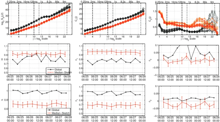
Fig. 4. Intra-day variability along the 3-day trace.For the 12 6h-blocks, comparisons of Global (black) and Median-Sketch (red) analyses: LDs (top); Estimated scaling exponents at CS (middle) and FS (bottom). Confidence intervals on Median-Sketch estimates are obtained as average across sketch outputs. For LDs (top), the ’+’ and the ’o’ correspond to night and day time estimates respectively. The dashed vertical lines mark respectively the typical IAT time scale JM
τ (blue), and the FS (black) and CS (dark grey) scaling ranges(j1, j2).
to 32s ([jCS
1 , j2CS] = [13, 18]), for years 2001-2006 and to
0.5s to 32s ([jCS
1 , j2CS] = [12, 18]) for years 2007-2014.
4) Fine Scales: Empirically, the Median-LDs indicate that scaling at FS holds up to roughly ∆F/2. While, obviously,
scaling cannot exist at scales finer than the IATτM,
Median-LDs clearly show that scaling holds right down to this scale. The fine scale range is thus given by
∆M
τ ≤ ∆ ≤ ∆F/2 or JτM ≤ j ≤ JF − 1.
In theory, scaling analysis implies that the different scaling parameters (H, c1, c2) are measured over the same scale range:
j1 ≤ j ≤ j2 for any given trace (or subtrace). However, the
practical computation of wavelet leaders, though mandatory to assess the departure of c2 from0, remains problematic at the
finest scales because to compute leaders at scale2j, one needs
wavelet coefficients at finer scales: As a consequence, wavelet leaders at the finest computed scales are biased (cf. [50] for detailed discussions) as can be seen in Fig. 2 (right plots). Thus, for simplicity and self-consistency, conservative FS ranges are selected so that all parameters are estimated over the same range. Because the IAT decreases significantly along the 14 years (cf. Fig. 3), inspections of Sketch-LDs lead us to choose[jF S
1 , j2F S] = [7, 10] corresponding to [16, 128]ms for
years 2001-2006, and [jF S
1 , j2F S] = [4, 10] corresponding to
[2, 128]ms over 2007-2014.
5) Partial Conclusion 2: Internet traffic scaling properties are characterized by a biscaling regime, corresponding to scaling in two distinct scaling ranges.
V. VARIABILITY ANDEVOLUTION OF
SCALINGWITHTIME
A. 3-Day Trace and Intra-Day Variability
Fig. 4 compares Global versus Median-LDs (and corresponding scaling exponents) estimated from the 12 non overlapping 6h-traces within the 3-day trace (top row). Global-LDs show a much larger variability, notably at CS, such that the use of Global-C2(j) becomes meaningless. In
fact, the scaling exponent estimates obtained from Global-LDs display a variability which is far too large for consistency with (bootstrap based) confidence intervals. Notably, the Global-LD estimates show a 24-hour periodicity, particularly clear at FS, that has (almost) disappeared from the Median-LD estimates. Beyond the potential natural diurnal cycle that could explain such modulation, inspection of traffic trace showed that the trinocular experiment, discussed earlier in Section II, was active during this trace. This anomalous traffic can be regarded as non stationary as it was essentially run at night (Japanese time), hence explaining the 24-hour periodicity. Further, the trinocular experiment sends, every 11 minutes, 1 to 15 ICMP probes to 3.4M blocks of IP addresses. Probes sent to the same block are spaced out by a 3 second timeout, thus producing a specific time scale in temporal dynamics that materializes as the bump atj ≃ 14 or 15 in Global-LDs (cf. Figs. 2 and 4). On average, Trinocular sends about 19.2 probes per hour per IPv4 block. It therefore produces a massive ICMP packet traffic superimposed to the
Fig. 5. Long term Evolution along the 14 years.For the 1176 15-min traces, Median-LDs (top) and comparisons between Global (black) versus Median (red)-based estimated scaling exponents at CS (middle) and FS (bottom).
remainder of the regular background traffic, thus significantly affecting traffic statistics and scaling properties at all scales. Global-LDs are hence polluted by this anomalous traffic, both at CS and FS, and their use would lead one to conclude that traffic undergoes a periodic modulation of its statistics and scaling properties, while this is actually due to the intermittent occurrence of the anomaly. Conversely, Median-LDs provide practitioners with a robust characterization of the background traffic, not altered by the trinocular anomaly. Median-LDs (and corresponding estimated parameters) display a remarkable constancy over time along the 3 days, thus showing the stationarity of intra-day statistical properties of Internet traffic, with minimal impact of the diurnal cycle.
Interestingly, a careful inspection of the Median-LDs for C2(j), Fig. 4 (top right), still shows a residual 24-h modulation
(C2(j) computed during 6-h day-time blocks differ from
those computed during 6-h night-time blocks). The Source IP Address has been chosen here as flow (hashing) key for sketching traffic. This allows trinocular (produced from a same IP Address) traffic to be concentrated into a single sketch output. However, this generates a response traffic, far lower in volume yet anomalous, which is not similarly concentrated. Robustness to that response traffic is indeed not achieved by hashing on Source IP Address, but would instead be obtained using Destination IP Address as the hashing key. In practice, one should thus ideally perform hashing on both Source and Destination Addresses. This indicates that LD C2(j)
corresponding to a refined and detailed analysis of statistical properties at all statistical orders, i.e., beyond correlation, may
thus be more impacted by remaining anomalous traffic than are LDsC1(j) and log2Sd(j), which essentially quantifies the
2nd order statistics. B. 15-Min Traces
Fig. 5 reports, for the 15-min traces, the Median-LDs (top) and compares the scaling exponents, as a function of trace collection time, estimated from Median-LDs to those of Global-LDs, for CS (middle) and FS (bottom). Global-LD estimates show a very large daily variability, far too large to be consistent with statistical estimation fluctuations. Common practice would trust such estimates, and lead to the (incorrect) conclusion that traffic scaling is not a robust property, as estimates keep changing. However, automated inspection of MAWI traces shows that there is almost no single day with-out significant anomalies [27], [59], [66], [67]. Global-LDs are thus essentially shaped by anomalous traffic. Conversely, Sketch-LDs (top row) and the corresponding estimated scaling parameters display a significantly reduced variability from one day to the next. Such variability is consistent with bootstrap-estimated statistical fluctuations, following procedures well-assessed in [50]. These observations constitute a significant indication for constancy of CS scaling over the 14 years.
Further, inspection of Fig. 5 shows an actual (mild yet clear) change in scaling exponents and scaling ranges, separating two roughly piecewise constant periods, from Jan. 2001 to June 2006 and from Oct. 2006 to Dec. 2014, respectively. Interestingly, summer 2006 corresponds to the link update, mentioned in Section II. This shows that a network
reconfiguration, even if major (significant increase of the available bandwidth), does not change drastically the general shape of the scaling properties in traffic (notably biscaling remains), but affects, though only marginally, scaling exponents and scaling ranges: Notably, ∆F and ∆τ
are both slightly decreased (cf. Fig. 3), which motivates the changes in the scaling range selection reported in Sections IV-B.3 and IV-B.4. The remaining variations of Median-LD estimates of H at both CS and FS, around years 2004-05 (cf. Fig. 5), correspond to the period of intense Sasser virus traffic. They show that once a given anomalous behavior becomes the dominant traffic, the sketch procedure considers it as the normal traffic and ceases to provide robustness against it [27].
C. Partial Conclusion 3
Median-LDs show unambiguously that Internet traffic exhibits remarkable constancy of its statistical and scaling properties, both at CS and FS, both for intra-day variability, with no impact of diurnal cycles acting as a nonstationary trend, and for long-term evolution: The scaling properties in MAWI traffic do not significantly change along the 14 years, neither in the shape of the LDs (biscaling is a robust property) nor even in the value taken by the scaling exponents, and this, despite the major changes undergone by the Internet during the last decade.
VI. NATURES ANDORIGINS OFSCALING
This section investigates the nature of scaling (LRD or multifractality), by systematically analysing scaling parameters H, c1 and c2 estimated off Median-LDs, at both
CS and FS. Potential mechanisms for the origins are also investigated quantitatively.
A. Coarse Scales
1) Nature of Scaling: For the 6-hour blocks of the 3-day trace, Median-LDs estimate H ≃ 0.92 ± 0.03, consistently along the 3 days (Fig. 4, middle left plot). This is consistent with the 15-min traces whereH is observed to remain confined in the range 0.8 ≤ H ≤ 1, with typical values around H ≃ 0.94 ± 0.03 after 2006, while H is found slightly lower H ≃ 0.86 ± 0.04 before 2006 (Fig. 5, middle left plot). Such values of H are extremely consistent with earlier measures on the same traffic [27] as well as on many other different traffics [1], [5], [18], [20], [54]. It is also consistently observed that c1 ≃ H and c2 ≃ 0 (see Figs. 4 and 5, middle row,
left plots) thus indicating no multifractality at CS. This is consistent with [20] that reported no evidence of multifractality on Auckland Traffic in an equivalent range of time scales. It is also interesting to note that besides the decrease of ∆F
(visible in Fig. 3, left), the link upgrade in 2006 has a fairly limited impact on scaling at CS.
2) Origins: As recalled in Section I, a mechanism was proposed to explain LRD in Internet Traffic, by relating it to the distribution of Internet object sizes via a generic heavy tail On/Off superimposition mechanism [1], [12]. In essence, this theoretical mechanism predicts asymptotic scaling in the
Fig. 6. Origin of scaling at CS: LRD versus heavy Tail. Flow size distribution (measured in pkt) show heavy-tail behavior, with tail exponent in exceptional quantitive agreement with Hurst exponent H at CS, as predicted in [12].
limit of very large scales: it is hence naturally associated to scaling at CS as defined in the present study. It, however, raises the issue of selecting the range of scales where LRD should be practically observed, in relation to heavy tails. As reported in Section VI-A, CS scaling extends up to a scale corresponding to data recording duration, and down to cut-off scale 2JF. These findings, associated with the typical
H ≃ 0.9, are in agreement with the methodological analyses of this asymptotic mechanism reported in [24], [42], and [64]. Further, the theorem in [1] and [12] predicts that, in the limit of CS, Internet traffic time series should be asymp-totically Gaussian self-similar, thus excluding multifractality (i.e.,c2≡ 0), again in agreement with empirical measurement
reported in the present study.
Despite the numerous efforts reported in the literature (cf. e.g., [13], [68]), a quantitative validation of the theoretical relation between heavy tail index α and H has turned out to be difficult to obtain from real measurements. This can been explained by practical difficulties in measuring the actual Internet object distribution and its corresponding index, as thoroughly documented in [24], [42], [64], and [68]. Following insights offered by the use of the Cluster Point process (CPP) model in [18], we explore here this generic link between LRD and heavy tail by studying the distribution of the flow sizes (in number of pkts). The estimation procedure for H and α, in particular in terms of selecting the ranges of scales and quantiles over which to conduct the linear regressions, carefully follows the methodology devised in [42] and [64]. The combined use of two methodological ingredients (multi-scale analysis and random projections) with the exceptional duration of Internet data (3-day trace), enables us to measure, on one hand H = 0.9 ± 0.05 for the pkt arrival process, and on other hand, α = 1.19 ± 0.05 as the tail index of the flow size distribution, as illustrated in Fig. 6. The theorem in [1] and [12] predicts a relation H = (3 − α)/2, which turns here into a remarkable match (3 − 1.19)/2 = 0.905 ± 0.025. To the best of our knowledge, this constitutes a quantitative agreement of unprecedented-quality between the theoretical prediction and empirical measures obtained on actual Internet traffic collected on real commercial links (see a contrario [42], [64] for simulated or Grid traffics).
3) Partial Conclusion 4: The present longitudinal study clearly shows robust and strong LRD with no multifractality for Internet traffic at CS, i.e., beyond 1s, moreover in close quantitative agreement with the tail exponent of flow size.
B. Fine Scales
1) Nature of Scaling: The parameter H measured at FS should theoretically not be referred to as the Hurst parameter, which is in essence associated to LRD, a CS property. Yet, H, measured as a scaling exponent across FS, preserves the key interpretation of accounting for a scaling property of the correlation, though within a finite range of (fine) scales. It is thus from now on labeled h, in reference to its link to the Hölder exponent, to which it should rather be associated in a multifractal setting (cf. e.g., [50]).
Fig. 4 (bottom row) shows that, for the 6-hour blocks of the 3-day trace, h ≃ 0.70 ± 0.02 and that c2 ≃ −0.025 ±
0.013, with clear departure from c2 = 0. Fig. 5 (bottom
row) shows that FS scaling parameters on the 15-min trace along the 14 years take roughly piecewise constant values in the two periods separated by the link upgrade mid-2006: h ≃ 0.57 ± 0.03, c2 ≃ −0.017 ± 0.012 before 2006, and
h ≃ 0.64 ± 0.03, c2≃ −0.044 ± 0.019 after 2006. For both
periods,H ≃ c1+ c2and the latter estimates are satisfactorily
consistent with those measured on the 3-day trace collected in 2013.
Global-LDs c2 are found close to 0 (both for the 6-hour
blocks of the 3-day trace and consistently for the 14 years of 15-min traces), which, if taken for granted, would lead to conclude that scaling at FS traffic is not multifractal, However, Median-LD c2 are consistently strictly negative
along the 14 years and for the 3-day trace, with confidence intervals either obtained by bootstrap or as an average across sketch outputs, excluding 0. This unambiguously suggests that Internet scaling at FS is better described by multifractal models, than by LRD ones. This is consistent with a number of contributions reporting multifractality in Internet traffic at scales of the order of 100ms on numerous different types of traffic and networks [14], [15], [25], [34], [35], [41], [42]. Conversely, [20] reported a lack of evidence for multifractality in Internet traffic. However, in all earlier studies (including ours [20]), multifractality was analysed without recourse to random projections that brings robustness, and with tools (such as wavelet coefficients or increments) that are now known to have a low ability to discriminate c2 < 0 from c2 = 0 and
thus are not good to unambiguously assess multifractality (see a contrario [41]).
2) Origins: Temporal burstiness of Internet traffic time series has been consistently reported, with bursts occurring over many different scales ranging from tens to hundreds of milliseconds (cf. e.g., [28], [47]). Multifractality naturally provides a relevant framework to model temporal burstiness (e.g., [37]). Fig. 5 (bottom right plot) further shows that the link upgrade in 2006 does not create nor obliterate multifractality at FS. Yet, the link update, and corresponding increase of bandwidth, induce a change in scaling parameters that, though not large in amplitude, appears as clear and robust: Stronger global structure in the correlation of Internet traffic at FS (increase of h and c1) with yet larger variability
beyond correlation, i.e., increased burstiness (increase of|c2|).
Multifractal scaling over FS constitutes an important statistical feature of Internet traffic, with notable impact of network performance (cf. e.g., [40], [69]). However, in contradistinction
to CS, no clear and well recognized mechanism has been proposed to explain scaling at FS.
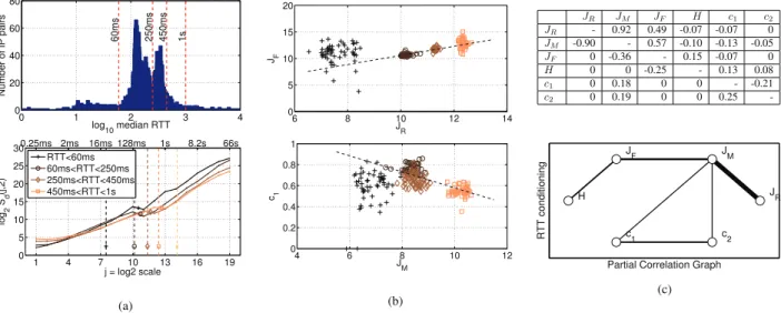
While scaling at CS has been related to flow sizes, scaling at FS has rather been associated to packet injection mech-anisms, that is essentially to the TCP congestion control, designed to regulate traffic. For instance, [47] described how TCP self-clocking shapes the packet interarrivals within TCP connections and thus the FS temporal dynamics. TCP has thus been envisaged as one of the mechanisms potentially producing or modifying burstiness and hence multifractality or scaling at FS [8], [15], [18], [33], [69]. The importance of time scales below the Round-Trip-Time (RTT) in Internet traffic temporal dynamics, has been evidenced (e.g. [47]). The relation and strength of scaling with respect to other queuing mechanisms (such as bottlenecks and congestions) has been further documented [16]. In [69], it was shown that protocol related burstiness contributed strongly to the form of the LDs over (what corresponds here to) FS, as did network topology aspects, albeit in a very simple dumbbell topology. In [70], it was shown that TCP congestion control can propagate scaling between distant areas of the Internet. In [42], varying TCP parameters was shown empirically to modify the scaling parameters measured at FS in Grid Traffic. TCP essentially relies on modifying a time window injection mechanism, depending on bandwidth availability and traffic congestion status: Large available bandwidth yields an additive increase of the slow-start window per returning acknowledg-ment packet, while loss detection results in a multiplicative decrease. This mechanism, linked to a cascade mechanism, has been envisaged in the context of Internet traffic in [37] and [70] as a potential explanation for multifractality, together with the protocol hierarchy of IP data networks [15], [69]. To quantitatively investigate the relations between the RTT induced time scale and multifractality at FS, RTT has been estimated for each flow using Karn’s algorithm [71], see also [72] for further details. Here, the difference between each TCP packet transmission time and the corresponding acknowledgment reception time is measured. Retransmitted packets are ignored to avoid ambiguous acknowledgments. The typical flow-RTT is estimated as the median of such RTTs. For one example 15-min trace, the empirical distribution of RTT estimates is reported in Fig. 7a and appears to be widely spread with several modes. Median-LDs are computed from subtraces designed by conditioning on RTT (partitioned in 4 classes as shown in Fig. 7a). They clearly suggest that the frontier scale ∆F = ∆02JF increases with RTT ∆R =
∆02JR. Fig. 7a also illustrates that the lower limit of the FS
range is controlled by the packet IAT.
This RTT-conditioning procedure is applied to 100 ran-domly chosen 15-min traces. Parameters H, h, c1, c2, JF are
estimated from the Median-LDs computed across the resulting 4×100 traces. For each of the classes, the median of JRis also
measured and its dispersion,JM, is estimated (as the median
absolute deviation). As expected theoretically, c1 and h are
highly correlated (ρ = 0.78) as they are essentially measuring the same dynamical property at the 2nd-order statistic level. The latter is thus removed from further analyses for clarity of exposition. The Graphical Gaussian Model framework [73]
Fig. 7. Origins of scaling at FS: RTT. (a) Top, empirical histogram of RTT, class-partitioning. Bottom, Median-LDs conditioned to RTT quantiles. The dashed-vertical lines correspond to the median RTT for each class of flows. LDs are normalized in amplitude for comparison. (b) Top: JF function of JR.
Bottom, c1 function of JM. The markers and colors of the data indicate the median RTT, as per the figure (a) bottom, on the left. (c) Top, Direct (upper
right triangle) and partial (lower left triangle) correlations between RTT distribution and scaling parameters. Bottom, corresponding Graphical Gaussian Model analysis of partial correlations.
is used to assess direct and partial correlations amongst the remaining 6 parameters. Partial correlation is classically used to quantify how much dependency remains between two vari-ables, once indirect correlations induced by the other variables are removed. This leads to the graph of relations reported in Fig. 7c and to the following comments and conjectures.
i) A weighted least square regression of JF against JR
(reported in Fig.7b) indicates that they are significantly corre-lated and that JF ≃ JR (or ∆F ≃ ∆R), in clear agreement
with daily-median RTT reported in Fig. 3 for the 1176 traces. Further, JF shows significant partial correlations with both
H and JM. RTT can be interpreted as a specific scale of
time, characteristic of a flow, and resulting jointly from inter-actions between available bandwidth, flow size and destination address. This typical time scale thus breaks the CS scaling induced by heavy tails thus creating the frontier scale JF,
whose value hence results from a competition between the CS heavy tail and the FS packet injection mechanisms.
ii) The median RTTs JR is strongly correlated to its
dispersion JM but shows negligible partial correlations with
any other scaling parameter. Conversely, the intra-class RTT dispersion JM shows significant partial correlations with all
scaling parameters. The large dispersion of RTTs (even within classes) implies that a broad spread of time scales contributes to temporal dynamics. A breadth of time scales, with no distin-guishable roles, contributing to temporal dynamics constitutes one potential known generic mechanism inducing scaling. Further, partial correlations suggest that JM acts as a hub
controlling the values of c1 (thus h) and c2. Negative direct
correlations (Figs. 7b and 7c) between c1 or c2 and both
JR and JM indicate that a decrease of JR and JM induces
largerc1 and|c2|. This confirms that the modulation of both
c1andc2also stems from the competing CS/FS mechanisms.
A decrease inJRandJM may be a consequence of an increase
in available bandwidth. For instance, the link upgrade in 2006, resulting into an increase of the available bandwidth, also implies a decrease in JF and JR. This bandwidth increase
makes possible a much more active and efficient TCP control mechanism, thus larger temporal burstiness and richer FS tem-poral dynamics, which are quantified by an increase of both c1 (stronger correlation) and|c2| (stronger multifractality).
iii) H at CS can be interpreted as not impacted by packet injection mechanisms and thus as solely depending on flow heavy tails.
3) Partial Conclusion 5: The present investigations provide robust evidence that the multifractal paradigm offers a relevant description of Internet traffic temporal dynamics at FS, notably accounting for burstiness, consistently along the 14 years studied here, as well as along the 3-day trace. They also report quantitative and consistent empirical evidence, relating the frontier scale∆F and FS temporal dynamics to RTT∆R
distributions, and thus to the TCP mechanism, in competition with the heavy tail CS mechanism.
VII. DISCUSSIONS ANDCONCLUSIONS
This longitudinal study over 14 years and across 3-days suggests the following comments and conclusions related to the scaling properties of Internet (MAWI) traffic, and echoing the challenges raised in Introduction section.
A relevant study of scale invariance in Internet traffic cannot be achieved without the combined use of multiscale representations and random projections. The latter permit statistical analyses that are robust to anomalous behaviors and thus describe background regular traffic. The former allow the range of scales where scaling behavior holds (through wavelet coefficients) to be determined and allows for a better discrimination of the nature of the scaling (wavelet leaders enable one to discriminate multifractality, beyond LRD).
Scaling properties in Internet traffic do exist and are not caused by spurious non stationarity. They develop not within a single scaling range but across two scaling ranges, the coarse and fine scales. This biscaling regime is a robust property that holds within traffic monitored continuously along the 3-day trace. This biscaling regime thus provides practitioners with a paradigm to describe the statistical properties of Internet traffic over scales from ms (10−3s) to several hours (104s), impressively ranging over 7 decades. This biscaling regime is also a property that has remained remarkably stable both in terms of the qualitative shape of LDs and in the values of the scaling exponents across the 14 years of the present study, thus showing that the amazing evolution of services, applications, behaviors and of technological capacity increase (bandwidth, volumes, …) have not caused any significant changes in the temporal dynamics of Internet traffic time series. Particularly, in contradistinction to what has sometimes been proposed (cf. e.g., [23], [26]), the present study shows that neither the increase in bandwidth and traffic volume nor the constant evolution of applications and services, have led to the disappearance of scaling properties. They favor neither the disappearance of LRD at CS, nor the return to Gaussian statistics and reduced burstiness at FS – multifractal properties remains.
The scaling at CS (above 1s) is well described by LRD that models temporal dynamics at the covariance (2nd order statistics) level, with no need for recourse to multifractality. As often proposed qualitatively, we showed here an exceptional quantitative agreement with the heavy tail behavior of the flow size (number of packets) distribution, providing an empirical validation of the universal mechanism proposed in [12]. This CS scaling holds up to the coarsest scale practically available for the analysis (several hours in the case of the 3-day trace) and remains visible down to scales of the orders of 0.5s where competing mechanisms related to within-flow packet injection become dominant. Details of the CS/FS competition, governing in particular the definition of the corresponding scale ranges, depend on RTT. This forms a link between scaling properties and protocol-specific mechanisms which can be further explored in future work.
In the FS regime, from several hundreds of ms down to the typical packet IAT (below 1ms), scaling temporal dynamics are better described by multifractal properties. Notably, while it is sometimes incorrectly associated to LRD, the burstiness of Internet traffic time series is actually well accounted for by multifractality: the larger |c2| (multifractality) the more
prominent the temporal burstiness. In contradistinction to CS, there is no universal mechanism proposed to described scaling at FS. Packet injection policies are driven by several protocols, the most prominent of which being TCP. TCP relies on a specific time scale, the RTT of a flow, that depends on flow size and destination, traffic volume and bandwidth. This study showed that the RTT distribution is very broad (see also [72]), thus producing a large continuum of time scales contributing to temporal dynamics and hence scaling. This study has provided quantitative evidence of the relations of scaling at FS with RTT. This is hence a possible mechanism producing scaling at FS, competing with scaling at CS, and thus producing the
biscaling regime. These links to RTT and TCP do not per se explain multifractality. Therefore, the point made in the present contribution is not that Internet traffic is multifractal at FS, but rather that multifractal processes constitute an efficient modeling of the statistics of Internet traffic at FS, notably accounting for temporal burstiness.
The frontier scale separating the two scaling regimes ranges from several hundreds of ms to1s. It can be regarded as a typ-ical time scale separating Internet users (human beings) gen-erating/producing the contents transferred through the Internet and hence to some large extent, the heavy tail of flow size, and technological behaviors (packet injection protocols).
Instead of having recourse to a different description for each scaling range, with no relation between the two ranges, one may prefer to use a single model valid across all scales (cf. e.g., [28] for the definition of an index of variability across all scales). The Cluster Point Process model (CPP), put forward in [18], provides a unique description of traffic across all available scales in a hierarchical manner (clusters of point processes) that accounts for flows and packets with-in flows. By construction, the CPP model is asymptotically LRD at CS when cluster size is heavy tailed, but being a point process cannot be strictly multifractal in the limit of FS. However, the extent to which it is well approximated as such across a large range of FS is currently being investigated. While theoretically appealing to describe Internet traffic, the CPP model is fully parametric hence less versatile to accommodate real data. Multifractal, and scaling exponents c1 and c2, can thus be
envisaged as alternative versatile semi-parametric features, practically, relevant and useful for various network tasks (e.g., traffic characterization and anomaly detection, cf. e.g., [53]).
ACKNOWLEDGMENT
P. Abry gratefully acknowledges the National Institute of Informatics for recurrent Visiting Professor funding.
REFERENCES
[1] W. E. Leland, M. S. Taqqu, W. Willinger, and D. V. Wilson, “On the self-similar nature of Ethernet traffic (extended version),” IEEE/ACM
Trans. Netw., vol. 2, no. 1, pp. 1–15, Feb. 1994.
[2] V. Paxson and S. Floyd, “Wide area traffic: The failure of Pois-son modeling,” IEEE/ACM Trans. Netw., vol. 3, no. 3, pp. 226–244, Jun. 1995.
[3] A. Erramilli, O. Narayan, and W. Willinger, “Experimental queueing analysis with long-range dependent packet traffic,” IEEE/ACM Trans.
Netw., vol. 4, no. 2, pp. 209–223, Apr. 1996.
[4] W. Willinger, M. S. Taqqu, R. Sherman, and D. V. Wilson, “Self-similarity through high-variability: Statistical analysis of Ethernet LAN traffic at the source level,” IEEE/ACM Trans. Netw., vol. 5, no. 1, pp. 71–86, Feb. 1997.
[5] P. Abry and D. Veitch, “Wavelet analysis of long-range-dependent traffic,” IEEE Trans. Inf. Theory, vol. 44, no. 1, pp. 2–15, Jan. 1998. [6] J. Beran, Statistics for Long-Memory Processes. New York, NY, USA:
Chapman & Hall, 1994.
[7] K. Park and W. Willinger, Self-Similar Network Traffic and Performance
Evaluation. Hoboken, NJ, USA: Wiley, 2000.
[8] A. Erramilli, M. Roughan, D. Veitch, and W. Willinger, “Self-similar traffic and network dynamics,” Proc. IEEE, vol. 90, no. 5, pp. 800–819, May 2002.
[9] I. Norros, “A storage model with self-similar input,” Queueing Syst., vol. 16, no. 3, pp. 387–396, Sep. 1994.
[10] O. J. Boxma and V. Dumas, “Fluid queues with long-tailed activeity period distributions,” CWI, Amsterdam, The Netherlands, Tech. Rep. PNA-R9705, Apr. 1997.


![Fig. 6. Origin of scaling at CS: LRD versus heavy Tail. Flow size distribution (measured in pkt) show heavy-tail behavior, with tail exponent in exceptional quantitive agreement with Hurst exponent H at CS, as predicted in [12].](https://thumb-eu.123doks.com/thumbv2/123doknet/14378550.505508/11.892.518.758.137.267/distribution-measured-behavior-exponent-exceptional-quantitive-agreement-predicted.webp)