HAL Id: hal-01691568
https://hal.archives-ouvertes.fr/hal-01691568
Submitted on 24 Jan 2018
HAL is a multi-disciplinary open access
archive for the deposit and dissemination of
sci-entific research documents, whether they are
pub-lished or not. The documents may come from
teaching and research institutions in France or
abroad, or from public or private research centers.
L’archive ouverte pluridisciplinaire HAL, est
destinée au dépôt et à la diffusion de documents
scientifiques de niveau recherche, publiés ou non,
émanant des établissements d’enseignement et de
recherche français ou étrangers, des laboratoires
publics ou privés.
Summarizing Large Scale 3D Point Cloud for Navigation
Tasks
Imeen Salah, Sebastien Kramm, Cédric Demonceaux, Pascal Vasseur
To cite this version:
Imeen Salah, Sebastien Kramm, Cédric Demonceaux, Pascal Vasseur. Summarizing Large Scale 3D
Point Cloud for Navigation Tasks. IEEE 20th International Conference on Intelligent Transportation
Systems, Oct 2017, Yokohama, Japan. �hal-01691568�
Summarizing Large Scale 3D Point Cloud for
Navigation Tasks
Imeen Ben Salah
*, S´ebastien Kramm
*, C´edric Demonceaux
†and Pascal Vasseur
**Laboratoire d’Informatique, de Traitement de l’Information et des Syst`emes
Normandie Univ, UNIROUEN, UNIHAVRE, INSA Rouen, LITIS, 76000 Rouen, France
†Laboratoire LE2I FRE 2005, CNRS, Arts et M´etiers, Univ. Bourgogne Franche-Comt´e
Abstract—Democratization of 3D sensor devices makes 3D maps building easier especially in long term mapping and autonomous navigation. In this paper we present a new method for summarizing a 3D map (dense cloud of 3D points). This method aims to extract a summary map facilitating the use of this map by navigation systems with limited resources (smartphones, cars, robots...). This Vision-based summarizing process is applied in a fully automatic way using the photometric, geometric and semantic information of the studied environment.
I. INTRODUCTION
Last years, the introduction of High-Definition (HD) and semantic maps has made a great participation in the large commercial success of navigation and mapping products and also in the enhancement of data fusion based localization algorithms. Several digital map suppliers like TomTom and HERE are now providing HD maps with higher navigation accuracy, especially in challenging urban environments. On the one hand, these HD maps provide more detailed representation of the environment even within large-scale 3D point cloud data. On the other hand, they require a high processing capacity with severe time constraints as well as a large storage requirement. Hence the need to find a new method to sum-marize these maps in order to reduce the required resources (computation / memory) to run the intelligent transportation systems while preserving the essential navigation information (saliency pixels, important nodes, etc.).
II. PREVIOUS WORKS
In some navigation tasks, setting a full-size map on a mobile device (car, robot, etc.) poses several difficulties. Appearance-based navigation methods are Appearance-based on global features like color, histogram or local features like points. To simplify the process of appearance-based navigation, a selection process is applied to select the key/reference features in the environment. In the visual memory approach a set of relevant and distinctive areas (images) are acquired and used during navigation by comparing it to the current position. This approach could serve to produce a compact summary of a map [9], [15], [16]. In the work of Cobzas [3], an example of panoramic memory of images is created by combining the acquired images with the depth information extracted from a laser scanner. In this image database, only the essential information to the navigation process will be retained [2]. This allows to obtain homoge-neous results with the same properties (precision, convergence,
robustness,. . . ) as the original global map. In order to build this image database, some techniques have been developed in order to guarantee the maximum efficiency in the choice of useful information. A spherical representation has been proposed by M. Meilland et al. [5], [13], [14]. This spherical representation is build by merging different images acquired by a set of cameras with the depth information extracted from a laser scanner. In this representation, all the information necessary for localization is present and compacted in a single sphere, thus avoiding the mapping of areas unnecessary to navigation [14]. We build upon this idea in this paper, as this approach is promising. Methods based on Bag of Words (BoW) are widely used for localization. BoW methods can efficiently represent a huge amount of data using the occurrences of several visual vocabulary. By applying hierarchical dictionary to the visual navigation problem [19], BoW methods proved a high scalability and accuracy in vision-based localization and mapping processes. The huge number of 3D points in HD maps makes point cloud compression algorithms essential for efficient storage and transmission. Over the past decade, several compression approaches have been proposed in lit-erature. Some of them employ special data structures such as octree [4] [6] for progressive encoding of point clouds. Schnabel et al. [17] propose a prediction scheme to achieve the compression using the octree approach. A novel compression method has been proposed in [10] to code only the spatial and temporal differences within an octree structure. Jae-Kyun
et al.[1] proposed a geometry compression algorithm for large
scale point cloud to encode radial distances in a range image. Several approaches based on feature selection to summarize a map for localization purposes were presented in [23], [24], [25]. The authors propose a few scoring functions to order the map landmarks according to their utility or to the observation statistics while guaranteeing a maximum coverage of the scene. An approach to map reduction was proposed in [26]. It aims to select only the places that are particularly suitable for localization using the location utility metric.
The remainder of this paper is organized as follows. First, we present an overview of our system. Next, we describe precisely our method for map summarization. Before conclud-ing our work in the last section, experiments and results are presented for a small point cloud and then for a large-scale labelled point cloud.
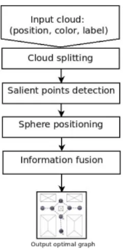
Fig. 1: Summarizing Large Scale 3D Point Cloud
III. OUR SOLUTION
Our work aims to perform several navigation tasks using only a map summary of the environment. This map should be not only compact but also coherent with the perception of the agent. To provide this map summary, we propose a new method dealing with large-scale 3D point clouds. The output of our summarizing method is a set of interconnected spherical images. Our main contributions are:
∙ We introduce the concept of ViewPoint Entropy, which
is a measure of viewpoint's informativeness based on geometric, photometric and semantic characteristics. The ViewPoint Entropy is used to facilitate best viewpoint selection.
∙ Using ViewPoint Entropy, we formulate map
summariz-ing process as an optimization problem.
∙ We propose a new representation of summarized
localiza-tion map using augmented and labelled spherical images.
∙ We introduce a novel partitioning step in our scalable
summarizing algorithm to allow large-scale point clouds handling.
In Fig. 1, we present the main steps of our algorithm to find the optimal set of spheres.
A. Cloud Splitting
To treat a large-scale 3D point cloud, we choosed to apply ”Divide and Conquer” method. This algorithmic technique consists in:
∙ Divide : split an initial problem into sub-problems.
∙ Conquer : solve sub-problems recursively or directly if
they are small enough.
∙ Combine : merge the solutions of the sub-problems to
find the global solution of the initial problem.
In our case, we might manipulate a very large 3D cloud with high density of information representing a large part of an urban environment. This method is therefore the best-suited to our needs. The first step of our algorithm consists in splitting the large 3D cloud from the beginning into several subsets to determine the optimum position of the sphere representing
Fig. 2: Splitting Large-scale point cloud
each small region (subset). To do this, we have proposed a splitting method. This technique allows us to split the input cloud into several cells using a discrete set of points called ”germs”. These germs are the centers of the cells. To adequately split the input cloud, the centers must cover all the navigable areas in the cloud (zones of circulation for cars, bikes and pedestrians). To find the best set of centers, we randomly select several points from the cloud. A new point is added to the set of germs if it is far enough (about 3 or 4 meters in our case) from every one of them and it belongs to the navigable areas. This process will be repeated until there are no more points respecting the criteria of a germ. Fig. 2 shows an example of splitting a 3D point cloud.
B. Salient Points Detection
In our final representation of the large-scale 3D point cloud, the salient areas must be represented in a very efficient way. To select these areas, we use the concept of visual saliency very commonly used these last years. There are many algorithms used for the detection of 3D visual saliency in a scene. Here, we consider three possible approaches dealing with saliency in 3D point cloud. They are based on the distinction between the regions in a scene. These methods are distinguished with the type of input information (geometric and photometic) used to extract salient points. The first method was proposed in [18]. This method uses a 3D point descriptor called Fast Point Feature Histogram (FPFH) (Geometric-based saliency) to characterize the geometry of the neighborhood of a point. A point is considered as distinct if its descriptor is dissimilar to all the other descriptors of points in the cloud. This operation is carried out on two levels with different neighborhood sizes.
First, a low-level distinctness 𝐷𝑙𝑜𝑤 is computed to detect the
small features. Then, a value of association 𝐴𝑙𝑜𝑤 is calculated
to detect salient points in the neighborhood of the most distinct
points. Next, a high-level distinctness 𝐷ℎ𝑖𝑔ℎ is computed to
select the large features. The final saliency map is calculated
for each 3D point 𝑝𝑖 as follows:
𝑆(𝑝𝑖) =
1
2(𝐷𝑙𝑜𝑤+ 𝐴𝑙𝑜𝑤) +
1
2𝐷ℎ𝑖𝑔ℎ (1)
However, this method uses only the geometry of the scene without any other type of information such as colors. A new algorithm for detecting saliency in 3D point cloud was presented in a recent work [20] (Supervoxel-based saliency). This algorithm consists in exploiting the geometric features and the color characteristics together to estimate the saliency
Fig. 3: Database (ground-truth) -a- manual segmentation -b-sphere positioning
in a cloud of colored points. All the 3D points are grouped in several supervoxels and then a measure of saliency for each set is calculated using the geometrical and photometric characteristics of its neighbors. This process is applied on several levels. Based on the center-surround contrast, a mea-sure of the distinctness is computed for every cluster using its feature compared to each surrounding adjacent cluster's one.
The feature contrast 𝜌𝑖 of a given cluster C at a given level i
is calculated as follows:
𝜌𝑖(𝐶) = 𝜃𝜌𝑔𝑒𝑜(𝐶) + (1 − 𝜃)𝜌𝑐𝑜𝑙𝑜𝑟(𝐶) (2)
Where 𝜌𝑔𝑒𝑜 and 𝜌𝑐𝑜𝑙𝑜𝑟 denote the normalized geometric and
color feature contrast of the cluster C, and 𝜃 is a weighting pa-rameter which is empirically set to 0.5 in [20]. Another method has been proposed in the work of Leroy [11] (Supervoxels-rarity) based only on supervoxels rarity. For each supervoxel 𝑣
a measure of rarity 𝑆𝑖(𝑣) is calculated using only photometric
characteristics (3).
𝑆𝑖(𝑣) = −𝑙𝑜𝑔(𝑃𝑖/𝑁 ) (3)
At each color component 𝑖, a self-information of the
occur-rence probabilities of the supervoxel 𝑃𝑖 is obtained and 𝑁 is
the number of supervoxels. To evaluate the level of saliency captured by these methods, we have proposed to calculate a
criterion called in the literature: 𝐹𝛽 [12] . This criterion allows
to characterize the relevance of the information returned by each method. This measure is calculated as follows:
𝐹𝛽= (1 + 𝛽2) * (𝑃 𝑟𝑒𝑐𝑖𝑠𝑖𝑜𝑛 * 𝑅𝑒𝑐𝑎𝑙𝑙) 𝛽2* 𝑃 𝑟𝑒𝑐𝑖𝑠𝑖𝑜𝑛 + 𝑅𝑒𝑐𝑎𝑙𝑙 (4) 𝑅𝑒𝑐𝑎𝑙𝑙 = 𝑇 𝑃 (𝑇 𝑃 + 𝐹 𝑁 ) (5) 𝑃 𝑟𝑒𝑐𝑖𝑠𝑖𝑜𝑛 = 𝑇 𝑃 (𝑇 𝑃 + 𝐹 𝑃 ) (6)
∙ True Positive (TP): number of points reasonably classified
as relevant for localization
∙ False Positive (FP): number of points wrongly classified
as relevant for localization
∙ False Negative (FN): number of points wrongly classified
as irrelevant for localization
𝐹𝛽 score is the weighted harmonic mean of precision and
recall and reaches its best value at 1 and worst score at 0.
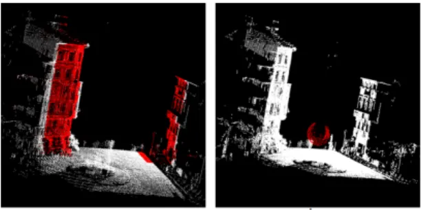
Fig. 4: Result of salient points detection according to the four 3D saliency extraction methods. -a- Geometric method [18] -b- Geometric and Photometric method [20] -c- Photometric method [11] -d- Harris3D [7] Methods 𝐹𝛽 Supervoxel-based saliency (𝜃 = 0.7) [20] 0.7401 Geometric-based saliency [18] 0.7234 Supervoxel-based saliency (𝜃 = 0.5) [20] 0.6696 Supervoxels-rarity [11] 0.5363 Harris3D [7] 0.4536
TABLE I: Results of salient points detection
Recall and precision are equally important if 𝛽 is set to 1. 𝛽 < 1 lends more weight to precision, while 𝛽 > 1 favors recall. To contrast the approach of using the maximum recall of points (no discrimination) we decided that precision should be given much more priority over recall. In our work, 𝛽 is set to 0.5 because it is one of the most common values assigned to 𝛽 (recall is half as important as precision).
C. Sphere Positioning
After completing the decomposition of the initial problem (large size) into a set of sub-problems (small size), we search for the optimal position of the sphere in a 3D cloud using optimization methods. This problem is known as Optimal point of view selection. In this type of problem, we aim to determine the best possible location of the Viewpoint in order to maximize the amount of information given by this sphere center. In the next part, we consider the map-summarizing process as an optimization problem.
1) Problem Modeling: Our goal is to determine the best
viewpoint allowing the capture of a maximum amount of salient points in the environment. This viewpoint will be represented by a spherical image. To find the optimal position of our sphere, we define a criterion called ”Viewpoint En-tropy”. The output of the entropy optimization process is a 3D
position (𝑋𝑜, 𝑌𝑜, 𝑍𝑜) of the optimal sphere center. To select
0.25 0.3 0.35 0.4 0.45 0.5 0.55 0.6 0.65 0 2 4 6 8 10 12 14 16 18 20 V iewP oint Entr opy Sampling step (10-5)
ViewPoint Entropy wrt Sampling step
Fig. 5: Entropy value of a given dataset related to the sampling step
use photometric, geometric and semantic information of the studied environment. This criterion is defined below.
Entropy Calculation
We consider {𝑃𝑖(𝑋𝑖, 𝑌𝑖, 𝑍𝑖, 𝑅𝑖, 𝐺𝑖, 𝐵𝑖, 𝐿𝑖), 𝑖 = 1..𝑁 } as
a finite set of N 3D points with their cartesian coordinates,
their labels 𝐿𝑖 and their colors (𝑅𝑖, 𝐺𝑖, 𝐵𝑖), and a point
𝐶(𝑋𝑐, 𝑌𝑐, 𝑍𝑐) as the center of our sphere. The idea is to
project all points of the cloud onto the sphere. For each point
𝑃𝑖, the coordinates (𝑋, 𝑌, 𝑍) of the projected point on the
sphere are: (︃ 𝑋𝑐 + 𝑅(𝑋𝑖− 𝑋𝑐) ‖ ⃗𝑃 𝐶‖ , 𝑌 𝑐 + 𝑅(𝑌𝑖− 𝑌 𝑐) ‖ ⃗𝑃 𝐶‖ , 𝑍𝑐 + 𝑅(𝑍𝑖− 𝑍𝑐) ‖ ⃗𝑃 𝐶‖ )︃ (7) Subsequently, we make the conversion into spherical coordi-nates:
(𝜑, 𝜃) = {︃
arccos(𝑍/𝜌)
arctan(𝑌 /𝑋) (8)
R is the radius of the sphere (set to 1 in our work). The next step is to sample these projected points to have a homogeneous points ditribution on all the spheres. To do this, we use constant angle sampling. In the real-time implementation of on-line localization algorithms, this type of sampling methods was used in order to favor the calculation time [13]. This method consists in sampling the projected points on the sphere:
𝑃𝑠=(𝜃,𝜑), with angles 𝜃 ∈ [−𝜋, 𝜋] and 𝜑 ∈ [0, 𝜋], using the
sampling steps 𝜕𝜃 et 𝜕𝜑
𝜕𝜃 = 2𝜋
𝑚, 𝜕𝜑 =
𝜋
𝑛 (9)
In this equation m denotes the number of samples in latitude and n the number of samples in longitude. We conducted a small study of the influence of the sampling step on the entropy value, regardless of other factors, on a given test dataset containing 60,000 3D points and representing an urban environment. The results are shown on Fig. 5. It appears
that it decreases strongly for values above 15 x 10−5 𝑟𝑎𝑑.
However, smaller values will increase the data volume thus we recommend staying with that value.
To obtain the corresponding intensity for each projected pixel, an interpolation is applied using the intensity of the nearest neighbor. We propose to define two levels of saliency
in a 3D point cloud. The low-level saliency 𝑆𝑙𝑜𝑤 is based on
low-level characteristics (photometric and geometric) of a 3D
point. The high-level saliency 𝑆ℎ𝑖𝑔ℎ is based on the semantic
information of each 3D point. To compute 𝑆𝑙𝑜𝑤 values we
use the Supervoxel-based saliency method described in the previous section which allows the combination of photometric and geometric information. We have chosen this method because it ensures a compromise between the calculation time and the selection of the most salient points useful for the
localization. To compute 𝑆ℎ𝑖𝑔ℎ values, we use the semantic
Labels for each point. Using these two types of saliency, we calculate the number of points of interest on the sphere according to their relevance. Therefore, we have four possible combinations as following.
∙ 𝑛00: number of non relevant points semantically,
photo-metrically and geophoto-metrically.
∙ 𝑛10: number of points relevant only photometrically and
geometrically.
∙ 𝑛01: number of points relevant only semantically.
∙ 𝑛11: number of points relevant semantically,
photometri-cally and geometriphotometri-cally.
The entropy of a sphere will be characterized by the entropy of its center P. The entropy is given by the algorithm 15: Algorithm 1 Entropy
Input :{𝑃𝑗(𝑋𝑗, 𝑌𝑗, 𝑍𝑗, 𝑆𝑗𝑙𝑜𝑤, 𝑆
ℎ𝑖𝑔ℎ
𝑗 ) ∈ S, 𝑗 = 1..𝑀 } ◁ 𝑀 is
the number of projected points on the sphere 𝑆 of center 𝐶
Output :𝜉(𝐶) ∈ [0..1]
1: procedure 𝜉(𝐶) ◁ The entropy of the center 𝐶
2: 𝜉(𝐶) ← 0 3: 𝑗 ← 1 4: 𝑛00← 0, 𝑛01← 0, 𝑛10← 0, 𝑛11← 0 5: for 𝑗 = 1 to 𝑀 do 6: if ((𝑆𝑗𝑙𝑜𝑤 = 0)𝑎𝑛𝑑(𝑆 ℎ𝑖𝑔ℎ 𝑗 = 0)) then 7: 𝑛00← 𝑛00+ 1 8: else if ((𝑆𝑙𝑜𝑤 𝑗 = 1)𝑎𝑛𝑑(𝑆 ℎ𝑖𝑔ℎ 𝑗 = 0)) then 9: 𝑛10← 𝑛10+ 1 10: else if ((𝑆𝑙𝑜𝑤 𝑗 = 0)𝑎𝑛𝑑(𝑆 ℎ𝑖𝑔ℎ 𝑗 = 1)) then 11: 𝑛01← 𝑛01+ 1 12: else 13: 𝑛11← 𝑛11+ 1 14: end if 15: end for 16: 𝜉(𝐶) ← 17: −𝑛00 𝑀 log 𝑛00 𝑀 − 𝑛01 𝑀 log 𝑛01 𝑀 − 𝑛10 𝑀 log 𝑛10 𝑀 − 𝑛11 𝑀 log 𝑛11 𝑀 18: return 𝜉(𝐶) 19: end procedure
2) Optimization: The Best Viewpoint Selection is an
en-tropy optimization process. This optimal point of view is the center of our optimal sphere. To maximize the entropy criterion, we have proposed a genetic algorithm to determine
the maximum of entropy function 𝜉 : 𝑋 → R3, where 𝑋
is the initial population of N 3D points. These points are the centers of the spheres on a navigable area in the cloud. This
Fig. 6: Result of spheres positioning according to the four 3D saliency extraction methods. -a- Geometric method [18] -b- Geometric and Photometric method [20] -c- Photometric method [11] -d- Harris3D [7]
optimization algorithm consists in evaluating the entropy of each member in the population. Both individuals (parents) with maximum entropy values are selected. The combination of two parents in a first iteration allows us to obtain a solution (child) with a better entropy than these parents. Thanks to this evolution of the viewpoint selection from one iteration to another, the algorithm becomes able to converge towards a solution among the points maximizing the entropy after a few iterations. The optimization algorithm is defined as follows: Algorithm 2 Genetic Algorithm
Inputs : Navigable area {𝑃𝑖(𝑋𝑗, 𝑌𝑗, 𝑍𝑗) ∈ Z, 𝑖 = 1..𝑁 }
Number of iterations 𝑁𝑖𝑡𝑒𝑟 Number of individuals 𝑁𝑖𝑛𝑑𝑖𝑣
Output :Best viewpoint 𝑉 ∈ 𝑍
1: procedure 𝐺𝐴(𝑍)
2: 𝑘 ← 1
3: 𝐼 ←Select 𝑁𝑖𝑛𝑑𝑖𝑣 random points ∈ 𝑍
4: while 𝑘 < 𝑁𝑖𝑡𝑒𝑟 do
5: for each point 𝑝ℎ in 𝐼 do 𝑒𝑛𝑡𝑟𝑜𝑝𝑦(ℎ) ← 𝜉(𝑝ℎ)
6: end for
7: 𝑝𝑎𝑟𝑒𝑛𝑡1 ← 𝑎𝑟𝑔 𝑚𝑎𝑥1(𝑒𝑛𝑡𝑟𝑜𝑝𝑦)
8: 𝑝𝑎𝑟𝑒𝑛𝑡2 ← 𝑎𝑟𝑔 𝑚𝑎𝑥2(𝑒𝑛𝑡𝑟𝑜𝑝𝑦)
9: for 𝑙 = 1 to 𝑁𝑖𝑛𝑑𝑖𝑣 do
10: Add 𝜆 * 𝑝𝑎𝑟𝑒𝑛𝑡1 + 𝛼 * 𝑝𝑎𝑟𝑒𝑛𝑡2 To 𝐼
◁ 𝜆 and 𝛼 random numbers ∈ [0..1]
11: end for
12: end while
13: return (𝑎𝑟𝑔 𝑚𝑎𝑥(𝑒𝑛𝑡𝑟𝑜𝑝𝑦))
14: end procedure
This algorithm has two parameters: maximum number of
iterations 𝑁𝑖𝑡𝑒𝑟 and initial population size 𝑁𝑖𝑛𝑑𝑖𝑣). To be
able to assign a value to them and maintaining a reasonnable computing time, we conducted a small study on some sample
dataset of 30 000 points. To find the optimal value of 𝑁𝑖𝑛𝑑𝑖𝑣,
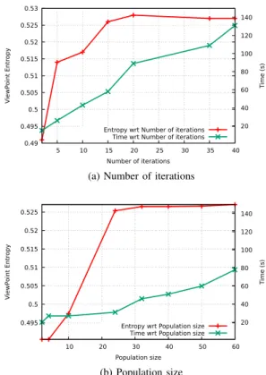
0.49 0.495 0.5 0.505 0.51 0.515 0.52 0.525 0.53 5 10 15 20 25 30 35 40 20 40 60 80 100 120 140 V iewP oint Entr opy Time (s) Number of iterations Entropy wrt Number of iterations
Time wrt Number of iterations
(a) Number of iterations
0.495 0.5 0.505 0.51 0.515 0.52 0.525 10 20 30 40 50 60 20 40 60 80 100 120 140 V iewP oint Entr opy Time (s) Population size Entropy wrt Population size
Time wrt Population size
(b) Population size
Fig. 7: Entropy and computation time values of a given dataset related to the population size and the number of iterations
we set 𝑁𝑖𝑡𝑒𝑟 to 5 and we measure the computation time and
the entropy value while varying 𝑁𝑖𝑛𝑑𝑖𝑣. Results can be seen
on Fig. 7a and show that values of 𝑁𝑖𝑛𝑑𝑖𝑣 above 20 give the
best results. However, higher values also increase computation
time. Similarly, Fig. 7b shows the he entropy value when 𝑁𝑖𝑡𝑒𝑟
varies while fixing 𝑁𝑖𝑛𝑑𝑖𝑣 = 20. It shows that values of 𝑁𝑖𝑡𝑒𝑟
above 15 are sufficient to reach a compromise between the algorithm convergence and the computation time.
D. Information Fusion
After the splitting and the sphere positioning steps, we will present, in this section, the last step of our algorithm allowing the calculation of the similarity between the obtained spheres. Then, the similar spheres are merged to eliminate the redundant information. This correlation (similarity) expresses the variation rate of the photometric, semantic and geometric information between every two compared spheres. In Meil-land's work [14], this criterion is calculated using the Median Absolute Deviation (MAD) which represents the difference (error) of intensity between the pixels of the two spheres (compared pixel by pixel). Similarly, we have proposed to
add a measure of semantic similarity 𝑆𝑠𝑒𝑚 between two
spheres. This measure aims to compute the number of similar pixels having the same label. We have also added a measure of geometric similarity by computing a histogram using the geometric descriptor FPFH. By comparing the histograms of different spheres we have obtained a measure of geometric
0.53 0.54 0.55 0.56 0.57 0.58 0.59 0.6 0 0.2 0.4 0.6 0.8 1 Fβ θ Fβ wrt θ
Fig. 8: Evolution of 𝐹𝛽of a given dataset related to the mixing
parameter 𝜃
Fig. 9: 3D point cloud Summary
similarity 𝑆𝑔𝑒𝑜𝑚.
𝑆𝑝ℎ𝑜𝑡= med(|𝑝(𝑥) − med(𝑝(𝑥))|)
𝑆𝑠𝑒𝑚= med(|𝑠(𝑥) − med(𝑠(𝑥))|)
𝑆𝑔𝑒𝑜𝑚= med(|𝑔(𝑥) − med(𝑔(𝑥))|)
𝑆 = 𝑚𝑒𝑎𝑛(𝑆𝑝ℎ𝑜𝑡+ 𝑆𝑔𝑒𝑜𝑚+ 𝑆𝑠𝑒𝑚) (10)
In this equations, 𝑝(𝑥), 𝑠(𝑥) and 𝑔(𝑥) are respectively the vectors containing the photometric, semantic and geometric errors between the pixels of the two spheres. Theoretically, two or more spheres are considered similar if the 𝑆 value is lower than a certain threshold. This is due to the small distance between the spheres. If two or more spheres are similar, a merging process is launched. This process consists in concatenating the two or more corresponding regions to the compared spheres and then re-applying the optimization method (Genetic Algorithm) in order to merge the similar spheres into one representing all the regions.
IV. RESULTS
A. Small 3D Point Cloud
At the beginning, we have tested our algorithm on a first database containing 60,000 3D points [21]. This point cloud,
developped originally without semantic information,
repre-sents an urban environment and covers around 400 𝑚2. We
have used this dataset to compare the 3D Saliency Extraction methods and to verify the estimated location of the optimal sphere. Because of its small size, this dataset is considered as a sub-part of a larger point cloud. Therefore, it was not necessary to apply the splitting step. We have chosen to implement and test the three methods detailed in the second section and the Harris3D [7] to extract a saliency map. We have compared the 3 methods, as detailed in the previous section, and also the method of interest points detector Harris3D known for its simplicity and efficiency in computer vision applications.
In order to build a ground-truth map before comparing these methods, we have manually segmented this urban database by choosing the most salient and useful points for localization. Among these points, we have selected those belonging to the building facade (front), the road signs and the ground marking. This ground-truth allowed the evaluation of the obtained results. Fig. 4 shows the result obtained by each
method. Table I shows the 𝐹𝛽 values obtained by the four
methods. The two algorithms using geometry to compute the saliency map had given better results than methods using only photometry because, in our case, points of interest for localization are generally more salient geometrically than photometrically. Fig. 6 shows the result of positioning the sphere in this scene. These results are obtained using a genetic algorithm for entropy optimization. We have obtained four results in the form of a position (x, y, z) of the center of the sphere summarizing the scene. Fig. 3 shows our ground truth. The sphere of the ground-truth is computed using the optimization algorithm (GA) and the ground-truth saliency map as described above. This sphere is located at equi-distance of the buildings and we have judged it to be the best point of view to visualize all the points of interest in this scene. We have calculated euclidean distance between the resulting spheres of the four methods and the sphere of the ground-truth (table I) to determine which one is the closest to the ground-truth sphere. The results obtained with the methods using geometry are the closest to the ground truth. We have obtained a compression ratio around 87%.
B. Large-Scale 3D Point Cloud
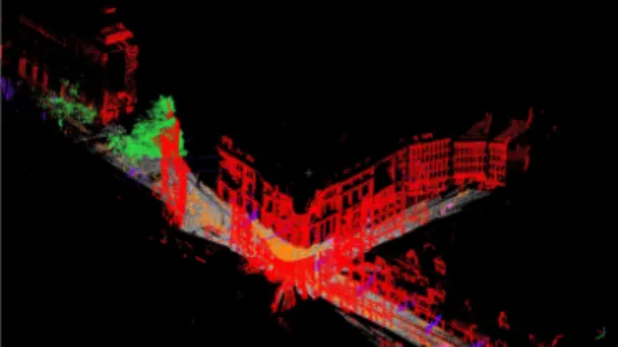
In the next part of our work, we have applied our method on a much larger environment. This large-scale point cloud contains over 40 millions of 3D labelled points [8]. In this dataset, we have 8 classes of labels (Fig. 10), namely {1: man-made terrain, 2: natural terrain, 3: high vegetation, 4: low vegetation, 5: buildings, 6: hard scape, 7: scanning artefacts, 8: cars}. An additional label {0: unlabeled points} marks points without any semantic value. In our summarizing pro-cess, points labelled ”buildings”, are considered among the most salient points for localization. This dataset permitted the evaluation of our solution's performance by using all semantic, photometric and geometric characteristics together. After splitting this large-scale point cloud, we have obtained 72 sub-clouds. To compute the saliency map we have chosen
Fig. 10: Semantic 3D Large-scale point cloud
the second method seeing that it provides a compromise between the relevance of the result and the time consumption. The parameter 𝜃 in equation 2 that controls the preference between geometric and photometric distinctness is assigned to a value of 0.7. This value has been chosen after a short study of the influence of the mixing parameter 𝜃 on the entropy value, on a small 3D Point Cloud described in the previous section. The results can be seen on Fig. 8 and clearly justify this value.
The output of this summary process, as shown in the Fig. 9, is a compact set of spherical images. We have obtained 35 spheres summarizing a point cloud of about 160 𝑚 length. The mean distance between all the spheres is around 4.5 𝑚. We have obtained a good compression ratio of this map (93%). To evaluate our solution, we have computed Recall and Precision (equations 5 and 6). They are defined as follows :
∙ True Positive (TP): number of relevant points actually
projected on the spheres
∙ False Positive (FP): number of irrelevant points actually
projected on the spheres
∙ True Negative (TN): number of irrelevant and
non-projected points on the spheres
∙ False Negative (FN): number of relevant and
non-projected points on the spheres
We have built our ground truth dataset. For each point in the cloud, we have attributed a label {0 : irrelevant for localization, 1 : relevant for localization}. Most of the relevant points belong to buildings thanks to their geometric shapes. As a result, we have significantly decreased the size of the map. Nevertheless, we have succeded to keep a maximum number of salient points (Recall around 60%) with a good level of precision (greater than 91 %). To improve the recall value, we could refine the input semantic labels to select the finest and most useful areas for localization (windows, doors, panels . . . ). All the spheres are positioned in a way to capture the maximum possible points belonging to the front facades of the buildings.
V. CONCLUSIONS
The developped method throughout this project allows us to summarize efficiently a large-scale point cloud. The summa-rizing process is based on the extraction of several spherical view representing sub-clouds of the initial map. This spherical
representation contains semantic, photometric and geometric information. This new method of summarizing 3D maps will allow us to facilitate several navigation tasks when applied in intelligent transportation systems (localization, route planning, obstacle avoidance, ...) by reducing significantly the calcula-tion time and the memory size required to the funccalcula-tioning of the navigation systems. We also believe that using the semantic information permits the development of a precise summary map by rejecting unnecessary localization data such us points belonging to dynamic objects (cars, pedestrians... ). Thanks to ”divide and conquer” technique, we have proposed a scalable summarizing algorithm dealing with large-scale point clouds. Our method outperforms existing systems. It enables the compressing of a 30,000 points cloud in less than 1 minute compared to 30 minutes as mentioned in [27]. In our future works, we will aim to provide a multilevel map in which a special level will be fully dedicated to every transportation system (trains, cars, bikes, pedestrians...) to enhance the navigation precision.
VI. ACKNOWLEDGMENTS
This work takes part in the ANR-15-CE23-0010-01 pLaT-INUM project. This project has been funded with the support from the French National Research Agency (NRA).
REFERENCES
[1] Jae-Kyun Ahn, Kyu-Yul Lee, Jae-Young Sim, and Chang-Su Kim. Large-scale 3d point cloud compression using adaptive radial distance prediction in hybrid coordinate domains. IEEE Journal of Selected Topics in Signal Processing, 9(3):422–434, 2015.
[2] Selim Benhimane, Alexander Ladikos, Vincent Lepetit, and Nassir Navab. Linear and quadratic subsets for template-based tracking. In IEEE Conference on Computer Vision and Pattern Recognition, pages 1–6, 2007.
[3] Dana Cobzas, Hong Zhang, and Martin Jagersand. Image-based local-ization with depth-enhanced image map. In Robotics and Automation, volume 2, pages 1570–1575, 2003.
[4] Olivier Devillers and P-M Gandoin. Geometric compression for interac-tive transmission. In Visualization 2000. Proceedings, pages 319–326. IEEE, 2000.
[5] Gabriela Gallegos, Maxime Meilland, Patrick Rives, and Andrew I Com-port. Appearance-based slam relying on a hybrid laser/omnidirectional sensor. In Intelligent Robots and Systems (IROS), pages 3005–3010, 2010.
[6] Pierre-Marie Gandoin and Olivier Devillers. Progressive lossless com-pression of arbitrary simplicial complexes. ACM Transactions on Graphics (TOG), 21(3):372–379, 2002.
[7] Chris Harris and Mike Stephens. A combined corner and edge detector. In Alvey vision conference, volume 15, page 50, 1988.
[8] IGP and CVG. Large-Scale Point Cloud Classification. Benchmark. http://www.semantic3d.net/, 2016.
[9] Matjaz Jogan and Ales Leonardis. Robust localization using panoramic view-based recognition. In Pattern Recognition, volume 4, pages 136– 139, 2000.
[10] Julius Kammerl, Nico Blodow, Radu Bogdan Rusu, Suat Gedikli, Michael Beetz, and Eckehard Steinbach. Real-time compression of point cloud streams. In Robotics and Automation (ICRA), 2012 IEEE International Conference on, pages 778–785, 2012.
[11] Julien Leroy, Nicolas Riche, Matei Mancas, and Bernard Gosselin. 3d saliency based on supervoxels rarity in point clouds.
[12] Ran Margolin, Lihi Zelnik-Manor, and Ayellet Tal. How to evaluate foreground maps? In IEEE Conference on Computer Vision and Pattern Recognition, pages 248–255, 2014.
[13] Maxime Meilland, Andrew I Comport, and Patrick Rives. A spherical robot-centered representation for urban navigation. In Intelligent Robots and Systems (IROS), pages 5196–5201, 2010.
[14] Maxime Meilland, Andrew I Comport, and Patrick Rives. Dense omnidirectional RGB-D mapping of large-scale outdoor environments for real-time localization and autonomous navigation. Journal of Field Robotics, 32(4):474–503, 2015.
[15] Emanuele Menegatti, Takeshi Maeda, and Hiroshi Ishiguro. Image-based memory for robot navigation using properties of omnidirectional images. Robotics and Autonomous Systems, 47(4):251–267, 2004.
[16] Anthony Remazeilles, Franc¸ois Chaumette, and Patrick Gros. Robot motion control from a visual memory. In Robotics and Automation, volume 5, pages 4695–4700, 2004.
[17] Ruwen Schnabel and Reinhard Klein. Octree-based point-cloud com-pression. In Spbg, pages 111–120, 2006.
[18] Elizabeth Shtrom, George Leifman, and Ayellet Tal. Saliency detection in large point sets. In IEEE International Conference on Computer Vision, pages 3591–3598, 2013.
[19] Fraundorfer, Friedrich and Engels, Christopher and Nist´er, David. Topo-logical mapping, localization and navigation using image collections. IROS, 3872–3877, 2007.
[20] Jae-Seong Yun and Jae-Young Sim. Supervoxel-based saliency detection for large-scale colored 3d point clouds. In IEEE International Confer-ence (ICIP), pages 4062–4066, 2016.
[21] Bernhard Zeisl, Kevin Koser, and Marc Pollefeys. Automatic registration of rgb-d scans via salient directions. In international conference on computer vision, pages 2808–2815, 2013.
[22] Whitley, L Darrell Foundations of genetic algorithms. morgan Kauf-mann, 1993.
[23] Marcin Dymczyk, Simon Lynen, Titus Cieslewski, Michael Bosse, Roland Siegwart, and Paul Furgale The gist of maps-summarizing experience for lifelong localization Robotics and Automation , 2015. [24] Muhlfellner, P., Burki, M., Bosse, M., Derendarz, W., Philippsen, R.,
Furgale Summary maps for lifelong visual localization Journal of Field Robotics, 2015.
[25] Hyun Soo Park, Yu Wang, Eriko Nurvitadhi, James C Hoe, Yaser Sheikh, and Mei Chen 3d point cloud reduction using mixed-integer quadratic programming Computer Vision and Pattern Recognition Workshops , 2013
[26] Ted J. Steiner, Guoquan Huang, and John J. Leonard Location utility-based map reduction obotics and Automation , 2015
[27] H. S. Park, Y. Wang, E. Nurvitadhi, J. Hoe, Y. Sheikh, and M. Chen, 3d point cloud reduction using mixed-integer quadratic programming Computer Vision and Pattern Recognition Workshops (CVPRW), 2013