HAL Id: hal-01545548
https://hal.archives-ouvertes.fr/hal-01545548v2
Submitted on 15 Jan 2018
HAL is a multi-disciplinary open access
archive for the deposit and dissemination of
sci-entific research documents, whether they are
pub-lished or not. The documents may come from
teaching and research institutions in France or
abroad, or from public or private research centers.
L’archive ouverte pluridisciplinaire HAL, est
destinée au dépôt et à la diffusion de documents
scientifiques de niveau recherche, publiés ou non,
émanant des établissements d’enseignement et de
recherche français ou étrangers, des laboratoires
publics ou privés.
Characterization: Application to Brain Tumors Using
Multiparametric Quantitative MRI Data
Alexis Arnaud, Florence Forbes, Nicolas Coquery, Nora Collomb, Benjamin
Lemasson, Emmanuel Barbier
To cite this version:
Alexis Arnaud, Florence Forbes, Nicolas Coquery, Nora Collomb, Benjamin Lemasson, et al.. Fully
Automatic Lesion Localization and Characterization: Application to Brain Tumors Using
Multipara-metric Quantitative MRI Data. IEEE Transactions on Medical Imaging, Institute of Electrical and
Electronics Engineers, 2018, 37 (7), pp.1678-1689. �10.1109/TMI.2018.2794918�. �hal-01545548v2�
Fully Automatic Lesion Localization and
Characterization:
Application to Brain Tumors using Multiparametric
Quantitative MRI Data
Alexis Arnaud, Florence Forbes, Nicolas Coquery, Nora Collomb, Benjamin Lemasson, and Emmanuel L. Barbier
Abstract
When analyzing brain tumors, two tasks are intrinsically linked, spatial localization and physiological characterization of the lesioned tissues. Automated data-driven solutions exist, based on image segmentation techniques or physiological parameters analysis, but for each task separately, the other being performed manually or with user tuning operations. In this work, the availability of quantitative magnetic resonance (MR) parameters is combined with advanced multivariate statistical tools to design a fully automated method that jointly performs both localization and characterization. Non trivial interactions between relevant physiological parameters are captured thanks to recent generalized Student distributions that provide a larger variety of distributional shapes compared to the more standard Gaussian distributions. Probabilistic mixtures of the former distributions are then considered to account for the different tissue types and potential heterogeneity of lesions. Discriminative multivariate features are extracted from this mixture modelling and turned into individual lesion signatures. The signatures are subsequently pooled together to build a statistical fingerprint model of the different lesion types that captures lesion characteristics while accounting for inter-subject variability. The potential of this generic procedure is demonstrated on a data set of 53 rats, with 36 rats bearing 4 different brain tumors, for which 5 quantitative MR parameters were acquired.
Index Terms
Perfusion imaging, Magnetic resonance imaging (MRI), Animal models and imaging, Computer-aided detection and diagnosis, Probabilistic and statistical methods, Automatic segmentation, Automatic characterization, Brain tumor, Quantitative multipara-metric MRI, Mixture model, Anomaly detection, Radiomics, Fingerprint model.
I. INTRODUCTION
M
AGNETIC resonance imaging (MRI) is the recommended imaging modality for brain tumor analysis (De Angelis [1], Drevelegas and Papanikolaou [2], Wen et al [3]). Several sequences may be obtained from a single MRI exam. When diagnosis is required, the radiologist is then left with a potentially large number of information sources but relatively few analysis tools. In this work, we propose an automated data driven tumor identification procedure where identification includes both localisation (segmentation) and characterization (signature). Segmentation is an intermediate Region-Of-Interest (ROI) determination step to produce tumor signatures that provide representations of the observed lesions with respect to their tissue composition. These compositions being characterized by various physiological parameters in good accordance with the expected tissue types. The construction of such signatures is made possible by the availability of so-called quantitative MRI. Quantitative MRI refers to maps of meaningful physical or chemical variables that can be measured in physical units and compared between tissue regions and among subjects. The use of such quantitative data has emerged more recently (see e.g. [4] and the journal issue on quantitative Brain MRI [5]). Most clinical MRI acquisitions rely on so-called weighted images, whose contrast is determined by a combination of different factors, tissue or experiment dependent. To detect pathology, conventional intensity-based MRI (e.g. Menze et al [6]) relies on differences in signal intensities which are not specific to the underlying biological state. Nevertheless, the term quantitative is often used when numeric values of signal intensities are measured and used for tissue segmentation and classification. We consider here a more stringent definition of the term quantitative as described in [5]. An important and promising aspect of quantitative MRI is the possibility to perform a meaningful analysis beyond a few global features such as mass diameter, the occurrence of an edema or of contrast enhancement. In addition, as the number and relevance of images increase, the sources of variability, such as inter-operator difference or subjectivity, should be carefully minimized but most current clinical practice lacks quantitative and reproducible assessment (Hectors et al [7], Menze et al [6], Weltens et al [8]).Several attempts, although less numerous than in conventional MRI analysis, have been made to analyze multiparametric quantitative MRI data to probe the information content of lesions. They usually consist of two steps, localization and charac-terization whose variability and accuracy can be controlled in two main ways respectively, through automated ROI selection
A. Arnaud and F. Forbes are with the Mistis team at Univ. Grenoble Alpes, INRIA, Laboratoire Jean Kuntzmann, Grenoble, France, E-mail: firstname.lastname@inria.fr. N. Coquery, N. Collomb, B. Lemasson, and E. Barbier are with Grenoble Institut des Neurosciences, Inserm U1216 & Univ. Grenoble Alpes, France, E-mail: firstname.lastname@univ-grenoble-alpes.fr.
and through quantitative feature extraction standardization. Most approaches focus on one or the other aspects: segmentation approaches are usually based on a few standard MRI maps, while more advanced feature extraction techniques commit to a preliminary manual ROI delineation. Coquery et al [9] propose to analyse 6 MR parameter maps and to identify different tissue types by looking for groups of voxels with similar parameter values. Voxels in manually segmented ROIs are clustered using a 6-dimensional Gaussian mixture model. The number of components (clusters) is chosen according to the Bayesian information criterion. Similarly, Boult et al [10] use manual segmentations followed by a k-means clustering of 3 MRI parameters maps to determine intra-tumoral tissue types whose relevance is assessed by comparison to histology data. In contrast, studies that focus on automated segmentation are generally faced with the issue of automatic lesion classes isolation. Unsupervised segmentation produces a partitioning into several classes with no clear semantic sense. Classes across different segmentations may not always represent the same tissue, complicating its biological interpretation. As an illustration, the intra-tumoral segmentation technique proposed by Katiyar et al [11] is restricted to a single tumor type localized and known in advance. These studies highlight the potential of conducting robust analysis from multiparametric quantitative data, but one common limitation is the number of tuning operations left to the user. Manual delineations have been already mentioned as an essential step, but most statistical inference procedures also rely on parameters that have to be set in advance such as the number of components in a mixture or the type of mixture distributions. Other limitations of the previous studies are that they do not account for dependencies between parameters or use multivariate Gaussian models because of their tractability in arbitrary dimensions and despite some observed parameter distributions have non Gaussian shapes [9]. In addition, the diagnosis ability of these approaches is not fully evaluated.
Therefore, there is a need for fully automated methods that can analyze multiple quantitative MR data in a reproducible way that correlates well with expert analyses.
A first challenge is the design of multivariate models that can capture non trivial interactions between physiological parameters while remaining tractable. The effort has to be put on the distributional modelling of the observed parameters whose deviation from standard Gaussian shapes may be of high significance. Similarly, extreme values of some of the parameters should be adequately modeled as important information may lie in the tails of the distributions rather than in their central part. For example, in human patients, glioblastoma are evaluated based on the high CBV (Cerebral Blood Volume) hotspot [12]. CBV values twice higher than that of normal appearing white matter are considered as originating from aggressive tumor tissue. To capture such non trivial interactions between multiple parameters, the usual multivariate Gaussian distributions but more generally the so-called elliptical distributions (Gaussian, multivariate Student, Laplace distributions, etc.) are limited by the type of elliptical shapes they allow. Observed physiological parameters seldom fit into such elliptical shapes (see Figure 1 below). Alternatives distributions, with a large variety of shapes, exist such as those using copula modelling [13]. Unfortunately copula models become rapidly intractable when more than 2 parameters have to be jointly modeled. When more than 2 parameters are available, it is important to design models that are both flexible in shapes and tractable in higher dimension. This is the case of the multiple scale t-distribution (MST) introduced in [14] which goes far beyond the standard Student distribution in terms of possible (not restricted to elliptical) shapes.
In addition to an accurate account of multiple parameters interactions, a second challenge is to perform accurate lesion localization. There are many ways to achieve lesion localization. The relevance of each of these ways depends on the available data. In this study we consider a weakly supervised case in which a moderate number of healthy (or control) subjects are available and identified as such. This automatically excludes deep learning methods that require a large amount of labelled voxels. Indeed, so far the most striking successes in deep learning have involved discriminative models and supervised classification tasks (see [15]–[17] and references therein). Models that have unsupervised learning capability with less requirement on ground truth labels are needed. Generative Adversarial Networks (GAN) [18] are unsupervised models that have been applied to natural images but have not been yet really assessed in a medical imaging context. Data augmentation and transfer learning, or the use of pre-trained networks, are promising directions of research but not quite mature yet. To our knowledge, there exists no pre-trained network or architecture for quantitative multi-modal medical images. Learning efficiently from limited data is still an important area of research. We believe more traditional unsupervised techniques are still useful to solve unsupervised tasks and to produce some proxy to the manual segmentations that are needed for neural networks. Among unsupervised segmentation methods, the vast majority of methods are clustering methods. But these are fully unsupervised and do not make use of the availability of a set of healthy subjects.
In our approach, we rather consider a novelty detection approach based on the identification of lesioned voxels as outliers with respect to a previously built reference model. Outlier detection can also be performed using a clustering approach (as in Van Leemput et al, 2001 [19], Gebru et al, 2016 [20] or Cuesta-Albertos et al, 2008 [21]) but most proposed methods are designed for only a few images per subject, usually less than 3. Detecting outliers in one dimensional data is less challenging than in multivariate data. In the multivariate case, the use of symmetric distributions may not be satisfying: the amount of outlying data has to be the same in each dimension, and this has no reason to occur in multi-contrast MRI data [22]. The proposed use of the MST distribution addresses specifically this problem. This is illustrated in Section III with statistical tests that reject Gaussianilty in both the healthy and pathological data cases. At last, one inconvenient of clustering approaches is that they usually require to use an atlas and to fix some sort of hyperparameters indicating for instance the expected number of outliers. In our novelty detection approach, we also have to set thresholds to distinguish intra-lesion classes but we propose
a data driven way based on model selection tools (for the determination of the number of classes) and extreme value theory (for the characterization of the thresholds as quantiles).
The approach proposed in the paper differs from existing work in various aspects. The use of flexible multivariate MST distributions allows to accumulate information from several (more than 3) physiologically meaningful parameters and therefore, successively 1) to build an accurate reference model from control subjects; 2) to perform automated lesion localization via novelty detection based on all imaged parameters but without the need of an atlas and hyperparameters tuning; and 3) to determine intra-lesion segmentations that can be turn into signatures and used to discriminate between different tumor types. The whole procedure is described in Section II and summarized in Figure 2. In Section III, its performance is illustrated on an independent evaluation data set.
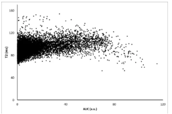
Fig. 1. Two observed physiological parameters: T2 vs AUC parameters for rats with C6 tumors. T2 and AUC values are plotted for each voxels in the tumors ROIs, illustrating skewness and different tail weights in the T2 and AUC directions. As expected, the permeability (i.e. AUC) measured in C6 tumors exhibits a large variability.
II. PROPOSED AUTOMATIC AND DATA-DRIVEN PROCEDURE
I
N the following developments, a generic and automatic data-driven procedure is described and its performance to segment and diagnose brain tumors without any high level expert or spatial knowledge is illustrated. The proposed procedure requires the availability of a dataset made of two sets of voxels: one from healthy subjects and one from pathological subjects for which the pathology (e.g. tumor) type is known. The considered features come from multiparametric quantitative MRI data that provides in each voxel a vector with several measures computed during the MRI session. Quantitative MR measures are considered, in particular, to be as independent as possible of the MRI scanner or the study center (Tofts [23]). In contrast to conventional MRI, image preprocessing issues such as bias field correction, resolution, etc. are less critical because parameters maps can be built so as to avoid most of these complications. For instance, in quantitative imaging, intensity bias is taken care of during the computation of parameter maps. In addition, the kind of data we consider here are acquired using the same geometry and at the same spatial resolution.The proposed procedure consists then of five steps: i) a first mixture model is fitted to the healthy subjects voxels; ii) this reference model is used to detect voxels which exhibit abnormal MR features with respect to the reference model, in the healthy and pathological subjects; iii) a second mixture model is fitted to the detected abnormal voxels and yields a clustering of these voxels into several classes; iv) the proportions of these classes in each subject are used as a signature of the pathology and a discriminative (fingerprint) model is learned that can distinguish between different pathology types; v) an additional spatial post-processing can be carried out to remove some spatial artifacts and refine the pathology signatures.
A. Reference model
Starting from a set of reference, typically healthy subjects, the goal is to construct a statistical parametric model of the MR parameters associated to these subjects. Each reference subject is associated to a number M of co-localized MR parameter maps that provide for each voxel v a M -dimensional vector of parameters denoted by yv. All voxels from all subjects are gathered
into a single set of voxels denoted by VH. The considered data set of M -dimensional vectors, pooling all vectors together, is
denoted by YH = {yv, v ∈ VH}. To characterize the distribution of these MR parameters, we consider a multivariate mixture
model to account for the potential heterogeneity in the parameter values due to the presence of different tissue types. This corresponds to cluster the data YH into a number of groups (clusters) of similar parameter vectors and to model each group
with a parametric distribution. In practice, in each dimension, the data are standardized to avoid scaling effects between MR parameters. This standardization is made at the whole dataset level and not for each subject individually.
In Coquery et al [9], a Gaussian mixture model is used assuming that each group is distributed according to a Gaussian distribution. However, the observed physiological parameters do not necessarily exhibit a Gaussian shape. Also Gaussian distri-butions are known to be sensitive to outliers whose occurrence may severely bias the estimation. As a more robust alternative, heavy tail distributions have the ability to accommodate potential outliers. In this paper, we consider such distributions and
Fig. 2. Construction of a model to automatically localize and characterize lesions. Starting from subjects labeled as healthy or pathological, the procedure is made of 5 main steps.
in particular multiple scale distributions (MST) introduced in Forbes and Wraith [14] that generalize the standard Student t-distribution. MST distributions allow the assignment of outlying parameter values to clusters without degrading the location and scale of the clusters. One advantage of the MST distribution over the standard t-distribution is a varying amount of tail weight in each dimension resulting in a much greater variety of distributional shapes. The mixture of MST distributions (MMST) that best fits the observed data YH is estimated using an Expectation-Maximization (EM) algorithm as described in Forbes and
Wraith [14]. This requires to set the number of groups in the mixture. This number, denoted by KH, is chosen automatically
from the data following a model selection approach. More specifically, we use the so-called slope heuristic (Baudry et al [24]) that generally provides a clear selection (see supplementary materials for more details). The clustering EM algorithm results in KH clusters, each represented by a multivariate M -dimensional MST distribution. Each distribution summarizes the MR
EM algorithm is that each voxel has a probability to be assigned to each cluster. The set of these membership probabilities can be seen as the signature of the voxel in the coding provided by the dictionary, the whole dictionary being itself summarized by the probability distribution function (pdf) of the estimated MMST model, namely
fH(y) = KH
X
k=1
πk MST (y; ψk) (1)
where MST (y; ψk) denotes the MST pdf with parameter ψk and proportion πk learned from YH. The pdf in (1) is referred
to as the reference model and will be used in the following anomaly detection step.
B. Anomaly localization
Considering a set of pathological subjects, the goal is to identify in each of them the lesioned voxels in order to provide a delineation of potential lesions. As lesions generally exhibit MR parameter values different from healthy tissues, lesion localization and delineation is recast into a novelty detection task. For a precise localization, mere visual inspection may not be enough and may be tedious when the number of available MR parameters increases. As before, the voxels of all pathological subjects are gathered into a set VP of voxels and the corresponding set of MR vectors is denoted by YP = {yv, v ∈ VP}. To
deal with comparable values, the normalization applied to the reference observations YH is also applied to YP. A voxel v is
considered as abnormal with regards to the previously built reference model fH in (1) if it corresponds to MR parameter values
yv with a low likelihood in the reference model. This likelihood is assessed via the reference pdf value at yv, i.e. fH(yv).
Novelty detection can be used not only to detect the lesioned voxels from the normal ones but among them to identify various degrees of proximity to normality. The log-density score log fH(yv) is considered as a measure of proximity of one voxel v
(associated to value yv) to the reference healthy model (represented by fH).
When considering the maps of all subjects, there are as many log-scores as there are voxels in the whole set of subjects. The idea is to look at the distribution of all these log-score values. As some of the voxels correspond to healthy tissues, there should be a group of voxels whose log-scores are high meaning a good adequacy with the reference model. More generally, we assume that there exist groups of voxels with similar log-scores and approximate the log-score values distribution as a MST mixture model. The number of groups L is determined automatically with the slope heuristic and a partition of the voxels into L groups is deduced. These groups can be ordered according to their mean log-score, from the farthest to the closest to the reference model. Then thresholds denoted by {t1, . . . , tL} are set to values that reflect the borders between two successive
groups. Among these thresholds, the topt threshold that corresponds to the retained lesion segmentation is just one of them.
The best 2-group partition of the log-scores is determined and the threshold that matches best with this partition is chosen as topt. For more explanations, see Appendix A. Figure 5 illustrates the obtained nested anomaly segmentations that reflect
different abnormality levels and are indicative of different tissue types within lesions. The global threshold topt can also be
used to separate the input data Y = YH∪ YP into a set of abnormal values YA and the rest:
YA= {yv, v ∈ VH∪ VP s.t. fH(yv) < topt} .
Note that, as the proposed thresholds are quantiles of the reference model pdf, healthy subjects may also exhibit a small fraction of abnormal voxels. Some of them are isolated voxels and can be easily removed using simple morphological operators (see Section II-E). However, these isolated voxels tend to be present in all subjects, for similar reasons (noise, skull stripping, artifacts, etc.), and their removal does not significantly affect the discriminative power of the fingerprint model. In contrast, other voxels may correspond to normal regions or structures (e.g. vessels, ventricles) whose physiological characteristics and then MR parameters are close to that of lesioned tissues. Individually, these voxels are therefore correctly detected as deviant from the reference model. However, their global signature is expected to be different from the signature of lesioned tissues and will then be learned by the fingerprint model.
C. Anomaly model
The goal of the two previous steps was essentially to perform automatic ROI localizations. The obtained ROIs provide a set of MR parameter vectors that are referred to as the abnormal data set YA. An anomaly model is then constructed following
the same procedure as for the reference model (Section II-A). The observations in YA are standardized in each dimension and
then used to fit a MMST model with a number KA of clusters selected with the slope heuristic. The fitted mixture is denoted
by fA, fA(y) = KA X k=1 ηk MST (y; φk) (2)
where MST (y; φk) denotes the MST pdf with parameter φk and proportion ηklearned from YA. This anomaly model is used
D. Fingerprint model
By fingerprint model we mean a model that can correctly characterize and classify a subject into one of a number of classes (e.g. different tumor types), based on MR parameters maps. Such a model is built in a supervised manner from pairs associating some chosen features to a class label. This requires the availability of a number of subjects for which the class label is known. The extracted features have then to be as informative as possible so as to allow the correct classification of unlabeled subjects. For each available subject in the learning data set, its anomaly class or label is known. These classes typically include the healthylabel and different tumor types. For each subject S, features are extracted from a set VS of nS voxels corresponding to
the voxels of S detected as abnormal in the previous step (Section II-B). As mentioned in Section II-B, healthy subjects also exhibit a small fraction of abnormal voxels. For each voxel v ∈ VS, the anomaly model (Section II-C) provides a probability
ρv
k that voxel v belongs to cluster k among KAclusters,
ρvk= ηkMST (yv; φk) PKA
l=1ηlMST (yv; φl)
.
For features at the subject level, we compute for each k = 1 : KA, the mean probability over voxels in VS,
ρSk = P v∈VSρ v k nS . The retained signature vector for subject S is then
ρS = {ρS1, . . . , ρ S
KA−1, nS} (3)
where the last probability has been removed and replaced with the ROI size nS to avoid co-linearity. Such a vector captures
the expression level of each anomaly cluster in the ROI of subject S. Intuitively, it is expected to capture the proportions of the different tissue types in the ROI. The addition of the ROI size seems natural at the stage as we suspect size could be discriminant if large number of pathologies and lesion types are considered. In the experiments on tumors made in Section III, size appears to be useful while not being essential to discriminate between different tumor types, as indicated by the similar ratios of the between-group variance over the total variance for each feature.
As for the supervised learning part, we adjust different discriminant analysis models and compare their ability to correctly predict the label (e.g. lesion type) of each subject by a leave-one-out cross-validation procedure. The selected discriminant analysis model is the one providing the highest true positive rate. Further details are given in the application Section III-D. E. Post-processing
The segmentations obtained in Section II-B can be further refined by removing connected components which are too small. This is done by applying an erosion-dilatation operator with a 9 voxels box-type kernel on each slice. In addition, the fingerprint model can improve the segmentations thanks to its ability to recognize healthy tissue. A fingerprint model is a signature definition as given in equation (3) (proportions of voxels in different groups) and a classifier able to distinguish between different signatures. A fingerprint model can then classify any ROI into a lesion type or as healthy. Therefore when a lesion is made of different connected components, these components can be seen as separated lesions for which a signature can be computed. Since signatures live all in the same space, whatever the size of the ROIs they are representing, the previously constructed classifier can be applied to classify each connected component separately. When a connected component is classified as healthy, we propose to remove it from the lesion. When doing this for all initial lesion segmentations, we obtain then (smaller) refined segmentations. Going back to the procedure described in Section II-D, the refined segmentations can in turn be used to relearn a refined classifier in two steps. First, since the removal of connected components may affect the different pixels proportions, signatures of the refined segmentations have to be recomputed. Then these new signatures can be used as input for the estimation of a new fingerprint model, referred to below as the refined fingerprint model. This post-processing enables the removal of groups of voxels that may individually exhibit MR parameter values close to lesioned tissues but show group anomaly proportions (signature) close to healthy components. After this stage, healthy tissues should correspond to a null signature (i.e. with no abnormal pixels) while the lesioned tissues signatures are cleaned from healthy tissues. An illustration is given in Figure 8.
F. Characterization and prediction
To predict the label of a new subject, its ROI is first determined using fH the reference model (Section II-A) for anomaly
detection (Section II-B). The obtained ROI is cleaned from potentially remaining healthy connected components that have not been removed by erosion-dilatation. The initial fingerprint model is used to identify these healthy connected components. The cleaned ROI (see Figure 6) is used to extract a ρS signature (see Figure 8) using the anomaly model (Section II-C) as explained in Section II-D. This signature is then given to the refined fingerprint model which provides an associated label (Table III).
TABLE I
AVAILABLE DATA:A LEARNING SET(Y = YH∪ YP)OF HEALTHY(YH)AND PATHOLOGICAL(YP) MRVALUES IS USED TO LEARNED A FINGERPRINT MODEL. ANOTHER TEST SET(YT)OF BOTH HEALTHY(YT
H)AND PATHOLOGICAL(YPT) MRVALUES IS USED FOR VALIDATION. THE SETS OF
DETECTED ABNORMAL VOXELS ARE ALSO INDICATED IN BOTH CASES(YAANDYAT). THE OBSERVATIONS DIMENSION IS5.
Learning set voxels subjects
Y = YH ∪ YP 260405 32 YH 45051 6
YP 215354 26 YA 57547 32
Test set voxels subjects
Y T = Y TH∪ Y TP 150085 21 Y TH 71340 11 Y TP 78745 10 Y TA 20105 21
O
UR procedure is illustrated on a data set of 53 rats for which 5 quantitative MRI maps are available. Some of the rats were implanted with different tumor types. The study design was approved by the local institutional animal care and use committee (COMETHS). All animal procedures conformed to French government guidelines and were performed under permit 380820 and B3851610008 (for experimental and animal care facilities) from the French Ministry of Agriculture (Articles R214-117 to R214-127 published on 7 February 2013). This study is in compliance with the ARRIVE guidelines (Animal Research: Reporting in Vivo Experiments [25]).A. Description of the MRI data
a) Rats and tumor types (Table I): The healthy subject group (YH) is composed of 6 healthy Fisher rats. The pathological
subject group (YP) contains 26 subjects with 4 tumor types: 9L (6 Fisher rats), C6 (6 Wistar rats), F98 (7 Fisher rats) and RG2
(7 Fisher rats). The MR parameter maps of all these subjects form the data set Y . For evaluation purpose, another group of subjects is available and contains 5 rats with 9L tumor, 5 rats with F98 tumor, and 11 healthy Fisher rats. The MR parameter maps associated to these subjects are kept as a test set and denoted by YT distinguishing the healthy sub-group YHT from the pathological one YPT.
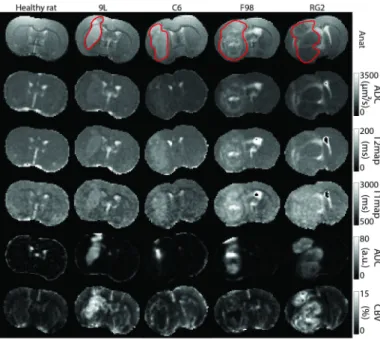
b) MRI parameters (Figure 3): The following 5 quantitative MR maps were acquired on 5 contiguous slices: apparent diffusion coefficient (ADC), T1, T2, CBV, and a vessel permeability map called area under the curve (AUC). All measures are naturally co-localized: all maps were acquired with the same geometry so that each voxel is described by the 5 parameters above. Section III-A in the supplementary materials provides further details about the MRI session. In addition, an anatomical T2-weighted image was acquired to allow automatic skull-striping. A manual delineation (superimposed red line in Figure 3 first row) of the tumor was performed using the anatomical image and the diffusion map. This manual segmentation is used as ground truth for the evaluation of the automatic tumor localization proposed in this study.
Fig. 3. MRI maps -ADC, T2, T1, AUC, CBV- associated to the central slice for one rat of each group (from the data set Y ). The red line superimposed on the anatomical map corresponds to the manual segmentation.
B. A healthy subjects based reference model
The reference model fH is built as a MMST model using an EM algorithm on the healthy subjects maps YH. When defining
this reference model, the slope heuristic approach selects KH = 10 clusters. An example of this partitioning in KH = 10
clusters is given in Figure 4 for the 5 slices of a healthy rat. In the whole set of healthy rats, 4 main clusters (red -1-, orange -2-, yellow -3-, light green -4-) gather 79.5% of the voxels in YH. The 6 remaining clusters (green -5-, turquoise -6-, blue -7-,
dark blue -8-, purple -9-, light purple -10-) correspond to less represented features such as vessels and ventricles (clusters 9 and 10) or interfaces between the main tissue types (interface between gray matter and cerebro-spinal fluid for clusters 6 and 7). Interestingly, although the model is adjusted without any spatial regularization, the resulting segmentations present spatially homogeneous regions and are rather visually consistent with brain anatomy: clusters 1 and 4 for the cortex and the corpus callosum, clusters 1 to 3 for the striatum, clusters 7 to 10 for the ventricles. The fitted MST distributions potentially include Gaussians that can be recovered by setting the degrees of freedom parameters to large values in the MST model [14]. To check that the fitted MST mixture does not reduce to a Gaussian mixture, the MST mixture component with the largest number of voxels was tested against Gaussianity using an Anderson-Darling test for each of the 5 parameters separately, (ADC, AUC, CBV, T1, T2). The respective p-values were (1.04e-06, 1.08e-01, 7.14e-24, 4.39e-15, 5.91e-19) indicating that only the AUC parameter could be considered as Gaussian, the probability of the data under the Gaussian distribution being less than 1e-06 for the other parameters. A similar conclusion was found with another statistical test referred to as the Shapiro-Wilk test.
Fig. 4. Reference model clustering (with KH= 10 clusters) on the 5 slices of one healthy rat. From left to right: slices in decreasing order along the vertical
axis of the scanner.
C. Anomaly localization
As described in Section II-B, for each MR parameter vector yv in Y , the pdf fH(yv) is evaluated. We found that these
values are best partitioned into 7 groups, according to the slope heuristic. Within each group, the voxels have similar likelihoods in the reference model, that is similar degrees of abnormality with respect to the reference model. This partition leads to 7 anomaly thresholds {t1, . . . , t7}. The optimal threshold that best divides the voxels into 2 subsets, according to a 2-component
mixture model (Section II-B), is the 4th threshold topt= t4. The abnormal subset YA= {yv, fH(yv) ≤ topt} represents 22.1%
of the full data set Y with a false positive rate of 1.4%, i.e. p(fH(Yv) ≤ topt) = 0.014 when the random variable Yv is
distributed according to the reference model. The voxels in YAform the subject ROIs.
An illustration is given in Figure 5-A last row. Colored voxels (thresholds t1 -red-, t2 -orange-, t3 -yellow- and t4 -green-)
belong to YA while grey ones (thresholds t5 -light grey-, t6 -medium grey- and t7 -dark grey-) are not tagged as abnormal.
The concordance with manual segmentation (superimposed red line in Figure 5-A) is indicated in Figure 5-B right via the computation of the Adjusted Rand Index (ARI) for each threshold. The higher the ARI the better, the maximum value being 1 (Rand [26], Hubert and Arabie [27]). For a given threshold tl, MR parameters yv in Y such that fH(yv) ≤ tl are selected.
The corresponding voxels form the segmentations linked to threshold tl, on which the ARI is computed. More specifically, the
ARI is computed at level tl for each rat. The boxplots in Figure 5-B show the variations of these ARI’s independently of the
tumor type. Other scores such as the DICE [28] are shown in Supplementary-Table III. Regarding global tumor delineation, it appears that the selected 4th threshold in the MMST case, corresponds to the best all tumor average ARI (0.42). ARI values can also be averaged for rats with the same tumor type. It appears then that some tumors are easier to segment. For instance, in the MMST case, for threshold t4, the average ARI’s are respectively of 0.49, 0.40, 0.32, and 0.47 for 9L, C6, F98 and RG2
tumors. The corresponding boxplots are shown in Supplementary Figure 5a. Inside the tumors, the thresholds also yield some satisfying spatial coherence. The strongest abnormality (red -t1- and orange -t2- areas in Figure 5) is mainly located at the
center of the tumor area. The delineated regions around (yellow -t3- and green -t4-) match with the border of the tumor area,
and the highest thresholds ({t5, t6, t7} -gray levels-) are mainly for the healthy voxels. However, it also appears that some
voxels are tagged as abnormal in healthy subjects (Figure 5-A 1st column) or in the contralateral part of pathological subjects (Figure 5-A 4 last columns). Based on their anatomical location, these voxels mainly correspond to ventricles and possibly blood vessels. As mentioned in Section II-E, most of these wrongly tagged voxels will be easily removed in Section III-D by using their signature after morphological operations. In terms of segmentation for the pathological rats, if we except the contralateral voxels, the 9L rat shows a high concordance with the manual segmentation, while the F98 segmentation is smaller and the RG2 segmentation is bigger. This is consistent with the intrinsic difficulty of delineating tumors of varying visual appearance across MR maps. As a matter of fact, on anatomical (Figure 5, 1st row) and diffusion images, 9L tumors are easier to delineate manually while F98 and RG2 tumors are more diffuse.
For comparison, our protocol is also applied with Gaussian mixture (GM) models. The anomaly localization results are shown in Figures 5-A, second row and B, left. The MMST model provides finer intra-tumoral descriptions with 4 abnormal
classes instead of 3 in the Gaussian case, and smoother segmentations. This is quantitatively confirmed by a MMST ARI of 0.42 which is 10.5% higher than the Gaussian ARI of 0.38. If healthy parts are considered instead, MMST and GM ARI are in the same order. Similar conclusions hold for the DICE values given in Supplementary-Table III. Regarding lesion segmentation, the main difference is in the contralateral areas. With GM models, the contralateral areas detected as abnormal are larger, and more of them are connected to the lesion areas, which leads to a less effective spatial post-processing. Indeed, only connected components not connected to the lesion area can be removed, because in case of contact the ROI signature does not correspond to the healthy one. As shown in Figure 6 for 9L and F98 tumors, the GM case requires more user interpretation than the MMST model to differentiate the lesion from the contralateral area.
Fig. 5. Nested anomaly segmentations for the different anomaly thresholds (part A), with the associated false positive rates and respective adjusted rand indices (part B) for the overlap with the manual segmentation. The thresholds are ordered from lowest (most abnormal in red) to highest (less abnormal in dark gray). The colored ones are those defining the abnormal data set YA. The gray ones correspond to normal groups. The ARI value for a threshold is
obtained by concatenating the segmentations associated to the thresholds lower to this threshold. The results are given for both Gaussian mixture and MMST models.
D. Anomaly and fingerprint models
A MMST model fA is adjusted on the abnormal YA data set with a number of clusters KA= 10 selected using the slope
heuristic. As in Section III-B, Anderson-Darling tests confirmed that the data did not exhibit Gaussian distributions with p-values of (3.70e-24, 3.70e-24, 3.75e-14, 4.62e-04, 3.58e-11) respectively for parameters (ADC, AUC, CBV, T1, T2). For each rat S in the learning set, we then extract a signature ρS as explained in Section II-D representing the proportions of each cluster in the ROI. The signatures are associated to the known subject labels in order to build a discriminative fingerprint model. Three discriminant analysis are compared based on their true positive rate with a leave-one-out procedure: linear discriminant analysis (lda: 90.6%, R package MASS, Venables and Ripley [29]), high dimensional discriminant analysis (hdda: 93.7%, R package HDclassif, Berg´e et al [30]), and a discriminant analysis based on a Gaussian finite mixture modeling (mclustda: 90.6%, R package mclust, Fraley et al [31]). The hdda analysis is retained due to its higher score to built a first fingerprint model. This fingerprint model is used in turn to refine the segmentations made in Section III-C. Too small connected components are removed with a 9 voxel box-type kernel and the fingerprint model is used to remove other connected components classified as healthy.
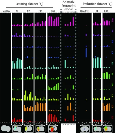
The obtained cleaned segmentations are illustrated for some rats in Figure 6. The ARI values for the 26 pathological rats in the training set are summarized in Figure 7 (boxplots), while mean DICE values are shown in Table II. Similar boxplots for DICE can be seen in Supplementary Figure 12. A signature for each subject is then computed using the cleaned ROI possibly still made of several connected components. The signatures are shown in Figure 8 for the 4 pathological groups and the healthy group. As a result of the post-processing, the healthy subjects present empty signatures. Although the four tumor models used in this study are aggressive glioma with a median survival of 3 to 4 weeks, the proportions of clusters differ between tumors. The 9L tumor is mainly composed of cluster 6 (turquoise), and to a lesser extent of clusters 1 (red), 3 (yellow), 9 (purple), and 5 (green). Cluster 6 is characterized by a high CBV and a mild edema as compared to normal tissue. This correspond to the high vascular density previously reported in 9L tumors [32]. The C6 tumor is mainly composed of clusters 2 (orange) and 3, and to a lesser extent of clusters 5, 1, 6 and 9. Clusters 2 and 3 are characterized by a high permeability and CBV values similar to that of normal tissue. This corresponds to the combination of low vascular density and large vascular diameter reported in [33] The F98 tumor is mainly composed of cluster 2, but also of clusters 3, 5, and 6.
Cluster 2 exhibits ADC, permeability, T1, and T2 values above that of cluster 3, and CBV below that of cluster 3, in line with [9]. Finally, tumor RG2 is mainly composed of clusters 1 and 4 (light green), and to a lesser extent of clusters 2, 3, 5, 6, and 7 (blue). Cluster 1 is characterized by its normal ADC and its high permeability and CBV as compared to normal values. This signature characterizes an angiogenesis without edema and corresponds to previous reports [34]. These results suggest that all tumors are heterogeneous and that different tissue types can lead to an aggressive tumor.
Fig. 6. Intra-tumoral segmentations for some of the pathological rats in the training set. First two rows: manual delineations and Gaussian clustering (KA= 13)
as described in [9]. Last two rows: Automatic segmentations and clustering using KA= 13 and KA= 10 with a Gaussian (3rd row) and MST (4th row)
mixture model. The ROIs correspond to the refined segmentation (i.e. after spatial post-processing).
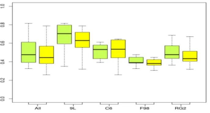
Fig. 7. Pathological rats in the training set: Adjusted rand index values per tumor type for the refined segmentations (i.e. after spatial post-processing), using the MMST (green) or Gaussian mixture (yellow) models.
TABLE II
PATHOLOGICAL RATS IN THE TRAINING SET: MEAN COVERING SCORES FOR LESION SEGMENTATIONS AFTER POST-PROCESSING USINGGAUSSIAN MIXTURE ANDMMSTMODELS.
Gaussian mixture model MMST model
9L C6 F98 RG2 All 9L C6 F98 RG2 All DICE index 0.677 0.636 0.665 0.823 0.704 0.718 0.644 0.677 0.833 0.721 ARI 0.607 0.509 0.386 0.466 0.487 0.661 0.514 0.409 0.507 0.518
E. Validation on a test data set
To evaluate the potential of our procedure, a test set different from the learning data set is used. It is composed of 9L rats (n = 5), F98 rats (n = 5), and healthy rats (n = 11). All voxels of these rats are gathered into data set YT. After
normalization with the normalization values used for the reference model, the pdf fH(yv) for each voxel v is computed and
values lower than topt define the abnormal voxels and subset YAT of Y
T. Each vector of parameters in YT
A is normalized
using the normalization values computed for the anomaly model fA. Individual subject signatures ρS are then first extracted
as described in Section II-D, eq. (3), for each rat in the test set. Spatial post-processing is then applied as explained in Section II-E to produce individual refined signatures on which are based the final predictions with the refined fingerprint model. All 9L rats are correctly predicted, but one F98 rat and one healthy rat are misclassified (Table III). The misclassified healthy rat, visible in Figure 8-right part, has only a few number of voxels tagged as abnormal (size, first line). Small differences on these
Fig. 8. Refined anomaly signatures by subject. Each signature is represented by a column with 10 rows (bars) indicated on the right hand side by K1 - K9 and Size. In each signature and each row, the bar corresponds to the proportion of voxels in the cluster corresponding to the row for the animal corresponding to the column. Left: individual subject refined signatures associated to the learning data set Y and grouped by tumor type. Center: mean signatures for each tumor type as provided by the refined fingerprint model. Right: individual refined signatures for each subject in the evaluation data set YT. For each tumor
type (9L, C6, F98, RG2) and healthy animals (H), an illustration of the segmentation is presented at the bottom.
few voxels may lead to very different signatures potentially closer to pathological ones. The misclassification of the F98 rat as a C6 rat may be explained by the C6 and F98 fingerprint models similarity: they share the same clusters but with different proportions. The Gaussian model faces the same difficulties to differentiate the C6 and F98 rats, with 3 miss-classifications. In contrast, all the healthy rats are well recovered (Table III). When manual segmentations are used like in [9], the confusion between F98 and C6 tumors is worse with all F98 rats classified as C6 rats both for the Gaussian mixture and MMST models. The refined segmentations for the evaluation data set test are presented in the Supplementary-Figure 13, with the associated values of ARI (Supplementary-Figure 14a) and DICE (Supplementary-Figure 14b). The average ARI and DICE scores are respectively 0.52 and 0.72.
TABLE III
TUMOR TYPE PREDICTION USING THE REFINED FINGERPRINT MODEL BUILT WITH THE TRAINING DATA SET(Y )AND EVALUATED ON AN INDEPENDENT TEST DATA SET(YT)FOR THEGAUSSIAN MIXTURE ANDMMSTMODELS BASED ON MANUAL OR AUTOMATIC SEGMENTATIONS.
Manual segmentation & Gaussian mixture or MMST model 9L C6 F98 RG2 Healthy Blind 9L (n=5) 5 . . . . Blind F98 (n=5) . 5 . . . Automatic segmentation & Gaussian mixture model
9L C6 F98 RG2 Healthy Blind 9L (n=5) 5 . . . . Blind F98 (n=5) . 3 2 . . Blind Healthy (n=11) . . . . 11
Automatic segmentation & MMST model 9L C6 F98 RG2 Healthy Blind 9L (n=5) 5 . . . . Blind F98 (n=5) . 1 4 . . Blind Healthy (n=11) . 1 . . 10
Q
UANTITATIVE MRI allows the comparison of measurements between subjects and with normative values acquired in a healthy population. The monitoring of subtle changes is then possible and represents an important component to design imaging biomarker candidates. In this study, a modular, fully automatic and data-driven procedure to detect and characterize abnormality within medical images was proposed. This procedure was tested on MRI data collected in rats bearing a brain tumor (4 tumor types). The lesions were localized within the brain as anomaly with respect to a reference probabilistic mixture model built using a dataset collected on healthy animals. Abnormal voxels were then clustered in groups with similar MR parameter values. The proportions of each group in each animal were used to construct a signature of each animal. For each tumor type, the signatures for the animals with this tumor type were used to build a fingerprint model of each tumor type. The specificity and sensitivity of the obtained fingerprints were eventually illustrated on a diagnostic task performed successfully without user interaction on an additional test data set. This first application of a procedure whose purpose is more general (any lesion visible by a radiologist, any type of clinical imaging modalities) relied on data from 4 tumor types and characterized by 5 quantitative parameter maps each. Six healthy rats and 26 pathological rats were used to learn the reference and pathology models and 21 additional rats were used for testing. While this dataset is large compared to other preclinical studies [9]–[11] and was sufficient to prove our concept (predictive rate greater than 90% in this particular application), it remains small compare to the volume of data collected daily in patients. Further evaluations are thus required on larger, pre-clinical and clinical data sets to confirm the robustness of the proposed method.One technical point of interest is that MST distributions performed better than Gaussian distributions: they yielded a better spatial agreement with the manual delineation (6.4% higher ARI on the learning set) and a better predictive rate (5.6% higher on the test set). While the quantitative MRI dataset obtained for tumor models and used in this study is probably not the most challenging one to compare the performance of the two distributions, the MST appears promising for its greater ability to accommodate outliers while maintaining a good separation between clusters [14].
The main evaluation criterion of our procedure was the final diagnostic. Further evaluations of the anomaly detection and of the anomaly model would also be useful to refine the procedure, including the number and type of MR parameter maps used to perform the automated diagnosis. To improve robustness, the results of the intermediate steps could be compared to that of histology. For our specific application (tumors), one could thereby evaluate the ability of MRI to detect abnormal cell densities and differentiate tissue types based on the standard pathologist diagnostic (Louis et al [35]). In addition to improving the quality of the procedure, the results of the intermediate steps may be of interest per se. The anomaly detection step, which progressively separates the tumor from the healthy tissue, could help neurosurgeons in planning a tumor resection (Barone, Lawrie and Hart [36]). The anomaly model, which discriminates tissue types, with specific parameter values (c.f. Supplementary Table IV), within the tumor, could be of interest to pathologists who cannot evaluate functional parameters such as blood flow. Clustering does not alter the types of information used as input. Thereby, radiologists or pathologists may directly interpret the output tissue characteristics, while such an interpretation is reportedly more difficult with deep learning techniques. Interestingly, the cluster maps show an excellent spatial coherence although no spatial information was used during the clustering steps of the procedure: all voxels were considered independent from each other. Moreover, at the lesion detection step, the ARI score reached 0.52 and the DICE 0.72 on the learning set, and respectively 0.49 and 0.69 on the test set (after post-processing in both cases). These scores were obtained from the comparison between a manual delineation performed on two images (anatomical and diffusion-weighted images as prescribed in standard clinical evaluation) and our procedure which used 5 parameter maps to delineate the tumor. As the images used to perform the delineations differed, it was not surprising to find different lesions between the automatic and the manual delineations. Histology could be used as a more reliable ground truth of high cell proliferation areas than manual delineation (De Angelis [1]). As in a clinical setting, it is generally not possible to obtain histological ground truth data on the entire tumor, this validation step has to be performed at a preclinical level.
The procedure proposed in this study is limited to the detection of tissues whose signal intensity (or parameter values) differs from that of normal tissue. However, a lesion may also appear as a tissue structure with a different volume (e.g. Alzheimer patients exhibit a reduction in the cortical thickness compared to age-matched, healthy, subjects [37]). While a large change in structure volume might be detected with our procedure as a change in the proportions of clusters in normal tissue, it would be of interest to add a spatial detection module based on a priori knowledge (e.g. atlas [22]). Moreover, a spatial regularization criterion could be added to the proposed procedure to exploit the fact that spatially close pixels have a higher probability to belong to the same tissue type [11], [38]. Exploiting complementarity between spatial proximity and parametric proximity should strongly reinforce our procedure. Once each subject of the training dataset has been labeled (healthy/pathology, lesion type) and the type of MR parameter maps chosen, the proposed procedure requires no human intervention. The determination of the optimal number of clusters, the anomaly threshold, and the final fingerprint model are data-driven to maximize the contrast between the reference data and the lesions and to best discriminate the tumor fingerprints.
In this respect, the proposed procedure differs from that in [9] and is a first attempt to combine both detection and characterization in an all-in-one procedure. It stands as an alternative to texture analysis in the context of radiomics [39]. In the context of multicentre studies, the mixture models at the heart of the procedure could be trained and controlled per center, thereby accounting for inter-center variability.
homogeneity, outliers) to obtain robust training datasets or to check the data set quality prior to performing an automated diagnostic. The proposed extensions would help meet the challenge of a human application in which the volume of data and number of tissue types represent an exciting challenge for the proposed computer-aided diagnosis procedure. Quantitative MR data are already available for humans [4], [5] but not standard however.
A follow up of this work would be to prove the feasibility and utility on human data with the hope then that quantitative images would be acquired on a more standard basis. To apply our method to more standard non quantitative MRI, one would need to decide on some normalization using for instance ideas from intensity normalization. The algorithm of Nyul et al, 1999 [40] is one of the most popular normalization techniques. Other recent approaches that would require further investigation are described in [41], [42]. Intensity bias correction would be more critically required and more attention should be put on inter-scanner variability [41].
APPENDIX A. Nested anomaly segmentations
A voxel v is considered as abnormal with regards to the reference model fH in (1), if it corresponds to parameter values yv
with a low likelihood fH(yv). Since pdf values cannot be interpreted as probabilities, the following key step is to decide on a
threshold toptbelow which voxels will be declared as abnormal, when fH(yv) ≤ topt. This threshold can be fixed to control the
false positive error, i.e. when Yv is distributed according to fH (healthy tissue), we seek for toptso that p(fH(Yv) < topt) = α
with a small value of α. However, the α value generally chosen (5%) is arbitrary and is likely not to coincide with lesions present in the data set. A threshold specific to the data under consideration is then preferable and can be computed as follows. Likelihood scores are computed for all voxels in VP, i.e. fH(yv), for all v ∈ VP, but also for the voxels that were used to
construct fH, i.e. fH(yv) for all v ∈ VH. Intuitively, high fH(yv) scores corresponding to parameters close to the reference
model should separate from the others. To fix the separation in a data driven way, we fit a MMST model to the log-score data set {log fH(yv), v ∈ VH∪ VP}. The slope heuristic is used to set the number L of components in the mixture. Due to
the heterogeneity of lesions, L is generally greater than 2 indicating the presence of abnormal tissues with different anomaly levels in the pathological data. Clusters can then be ordered according to their respective mean log-score. The lowest mean corresponds to a group whose departure from the reference model is the highest, while the highest mean should correspond to healthy voxels. The voxels are then partitioned into L groups of successive anomaly levels. Anomaly thresholds are set to the highest likelihood score in each group and denoted by {t1, . . . , tL}. They are used to provide nested anomaly segmentations
that reflect the structure of the lesions (e.g. Figure 5). For a global lesion segmentation, another MMST model is fitted to the log-scores with the number of groups set to 2. The two groups are ordered according to their means. For consistency with the previously computed thresholds, we retain as the global threshold toptthe value in the series {t1, . . . , tL} which is the closest
to the highest score in the first group of the 2-component mixture. The thresholds that correspond to abnormality levels are the ones lower or equal to topt, that is {t1, . . . , topt}. They are associated to colored voxels in Figure 5. For each of them,
we compute the false positive probability αl = p(fH(Yv) < tl) when Yv is distributed according to fH. Unfortunately the
distribution of fH(Yv) is usually not known and the αl’s need to be computed using simulations. However, the thresholds tl
correspond in general to extreme quantiles so that standard empirical estimation would lead to αl = 0 in most cases. For a
more precise estimation, we propose to use extreme value theory that enables a more accurate modelling of the distribution tail (see e.g. [43]). Details are given in the following Appendix B.
B. Extreme quantile estimation
The computation of α = p(fH(Y ) ≤ t) when Y follows fH is problematic because the pdf of fH(Y ) and its theoretical
quantiles are not available in general. Empirical estimates are easy to obtain via simulation of i.i.d. realizations of fH(Y ).
However, the t-values of interest are in general extreme quantiles and very few simulated values of fH(Y ) will be smaller
than t in practice so that α will be estimated to 0. This is a standard issue in extreme quantile estimation that can be addressed via extreme value theory (EVT). EVT focuses on distributions maxima and minima. Considering a set of i.i.d. variables {Zm,n, m =1:M, n =1:N }, a set {Z1∗, . . . , ZM∗ } of M maxima can be defined as Zm∗ = max(Zm,1, . . . , Zm,N). EVT provides
an estimation of the pdf denoted by f of the Zm∗s via the estimation the generalized extreme value (GEV) distribution. In
particular, most EVT procedures provide good estimations of p(Zm∗ ≤ η) when η is an extreme value in the upper tail of f .
Our task can then be recast as follows,
p(fH(Y ) ≤ t) = 1 − p(fH(Y ) > t)
with p(fH(Y ) > t) = p(min(fH(Y1), . . . , fH(YN)) > t)1/N
where {Y1, . . . , YN} are i.i.d. with distribution fH. Then
p(min(fH(Y1) . . . fH(YN)) > t) = p(max(−fH(Y1) . . . − fH(YN)) ≤ −t)
= p(max(− log fH(Y1) . . . − log fH(YN)) ≤ − log t) .
This latter quantity is computed setting η = − log t and Zi= − log fH(Yi). The log turns the bounded upper tail of −fH(Y )
into an unbounded upper tail in − log fH(Y ). This provides more stable estimation of the GEV parameters obtained here with
ACKNOWLEDGEMENTS
The authors acknowledge the excellent technical support of the MRI Facility of Grenoble (UMS IRMaGe). IRMaGe is partly funded by the French program Investissement d’Avenir run by the French National Research Agency, grant Infrastructure d’avenir en Biologie Sant´e[ANR-11-INBS-0006].
REFERENCES
[1] L. M. De Angelis, “Brain Tumors,” New England Journal of Medicine, vol. 344, no. 2, pp. 114–123, January 2001.
[2] A. Drevelegas and N. Papanikolaou, Imaging of Brain Tumors with Histological Correlations. Springer Berlin Heidelberg, 2011, ch. Imaging Modalities in Brain Tumors, pp. 13–33.
[3] P. Y. Wen, D. R. Macdonald, D. A. Reardon, T. F. Cloughesy, A. G. Sorensen, E. Galanis, J. DeGroot, W. Wick, M. R. Gilbert, A. B. Lassman, C. Tsien, T. Mikkelsen, E. T. Wong, M. C. Chamberlain, R. Stupp, K. R. Lamborn, M. A. Vogelbaum, M. J. van den Bent, and S. M. Chang, “Updated Response Assessment Criteria for High-Grade Gliomas: Response Assessment in Neuro-Oncology Working Group,” Journal of Clinical Oncology, vol. 28, no. 11, pp. 1963–1972, 2010.
[4] O. Wu, R. M. Dijkhuizen, and A. G. Sorensen, “Multiparametric magnetic resonance imaging of brain disorders,” Topics in Magnetic Resonance Imaging, vol. 21, no. 2, pp. 129–138, 2010.
[5] C. Pierpaoli, “Quantitative Brain MRI,” Topics in Magnetic Resonance Imaging, vol. 21, no. 2, p. 63, 2010.
[6] B. H. Menze, A. Jakab, S. Bauer, J. Kalpathy Cramer, K. Farahani, J. Kirby, Y. Burren, N. Porz, J. Slotboom, R. Wiest, L. Lanczi, E. Gerstner, M. A. Weber, T. Arbel, B. B. Avants, N. Ayache, P. Buendia, D. L. Collins, N. Cordier, J. J. Corso, A. Criminisi, T. Das, H. Delingette, C. Demiralp, C. R. Durst, M. Dojat, S. Doyle, J. Festa, F. Forbes, E. Geremia, B. Glocker, P. Golland, X. Guo, A. Hamamci, K. M. Iftekharuddin, R. Jena, N. M. John, E. Konukoglu, D. Lashkari, J. A. Mariz, R. Meier, S. Pereira, D. Precup, S. J. Price, T. R. Raviv, S. M. S. Reza, M. Ryan, D. Sarikaya, L. Schwartz, H. C. Shin, J. Shotton, C. A. Silva, N. Sousa, N. K. Subbanna, G. Szekely, T. J. Taylor, O. M. Thomas, N. J. Tustison, G. Unal, F. Vasseur, M. Wintermark, D. H. Ye, L. Zhao, B. Zhao, D. Zikic, M. Prastawa, M. Reyes, and K. Van Leemput, “The Multimodal Brain Tumor Image Segmentation Benchmark (BRATS),” IEEE Transactions on Medical Imaging, vol. 34, no. 10, pp. 1993–2024, October 2015.
[7] S. J. C. G. Hectors, I. Jacobs, G. J. Strijkers, and K. Nicolay, “Automatic segmentation of subcutaneous mouse tumors by multiparametric MR analysis based on endogenous contrast,” Magnetic Resonance Materials in Physics, Biology and Medicine, vol. 28, no. 4, pp. 363–375, 2015.
[8] C. Weltens, J. Menten, M. Feron, E. Bellon, P. Demaerel, F. Maes, W. van den Bogaert, and E. van der Schueren, “Interobserver variations in gross tumor volume delineation of brain tumors on computed tomography and impact of magnetic resonance imaging,” Radiotherapy and Oncology, vol. 60, no. 1, pp. 49–59, 2001.
[9] N. Coquery, O. Franc¸ois, B. Lemasson, C. Debacker, R. Farion, C. R´emy, and E. L. Barbier, “Microvascular MRI and unsupervised clustering yields histology-resembling images in two rat models of glioma,” Journal of Cerebral Blood Flow & Metabolism, vol. 34, no. 8, pp. 1354–1362, May 2014. [10] J. K. Boult, M. Borri, A. Jury, S. Popov, G. Box, L. Perryman, S. A. Eccles, C. Jones, and S. P. Robinson, “Investigating intracranial tumour growth
patterns with multiparametric MRI incorporating Gd-DTPA and USPIO-enhanced imaging,” NMR in Biomedicine, vol. 29, no. 11, pp. 1608–1617, 2016. [11] P. Katiyar, M. R. Divine, U. Kohlhofer, L. Quintanilla Martinez, B. Sch¨olkopf, B. J. Pichler, and J. A. Disselhorst, “A Novel Unsupervised Segmentation Approach Quantifies Tumor Tissue Populations Using Multiparametric MRI: First Results with Histological Validation,” Molecular Imaging and Biology, vol. 19, no. 3, pp. 391–397, 2017.
[12] M. Law, S. Yang, J. Babb, E. Knopp, J. Golfinos, D. Zagzag, and G. Johnson, “Comparison of cerebral blood volume and vascular permeability from dynamic susceptibility contrast-enhanced perfusion MR imaging with glioma grade,” American Journal of Neuroradiology, vol. 25, no. 5, pp. 746–755, 2004.
[13] I. Kosmidis and D. Karlis, “Model-based clustering using copulas with applications,” Statistics and Computing, vol. 26, no. 5, pp. 1079–1099, 2016. [14] F. Forbes and D. Wraith, “A new family of multivariate heavy-tailed distributions with variable marginal amounts of tailweights: Application to robust
clustering,” Statistics and Computing, vol. 24, no. 6, pp. 971–984, 2014.
[15] Z. Akkus, A. Galimzianova, A. Hoogi, D. L. Rubin, and B. J. Erickson, “Deep Learning for Brain MRI Segmentation: State of the Art and Future Directions.” Journal of Digital Imaging, vol. 30, no. 4, pp. 449–459, 2017.
[16] G. Litjens, T. Kooi, B. E. Bejnordi, A. Arindra-Adiyoso-Setio, F. Ciompi, M. Ghafoorian, J. A. van der Laak, B. van Ginneken, and C. I. S´anchez, “A survey on deep learning in medical image analysis,” Medical Image Analysis, vol. 42, pp. 60–88, 2017.
[17] D. Shen, G. Wu, and H. Suk, “Deep learning in medical image analysis,” Annual Review of Biomedical Engineering, vol. 19, pp. 221–248, 2017. [18] I. J. Goodfellow, J.Pouget-Abadie, M. Mirza, B. Xu, D. Warde-Farley, S. Ozair, A. C. Courville, and Y. Bengio., “Generative adversarial nets.” in Advances
in Neural Information Processing Systems 27: Annual Conference on Neural Information Processing Systems 2014, Montreal, Quebec, Canada, 2014, pp. 2672–2680.
[19] K. van Leemput, F. Maes, D. Vandermeulen, A. Colchester, and P. Suetens, “Automated segmentation of multiple sclerosis lesions by model outlier detection,” IEEE Transactions on Medical Imaging, vol. 20, no. 8, pp. 677–688, 2001.
[20] I. D. Gebru, X. Alameda-Pineda, F. Forbes, and R. Horaud, “EM algorithms for weighted-data clustering with application to audio-visual scene analysis,” IEEE Transactions on Pattern Analysis and Machine Intelligence, vol. 38, no. 12, pp. 2402–2415, 2016.
[21] J. A. Cuesta-Albertos, C. Matran, and A. Mayo-Iscar, “Robust estimation in the normal mixture model based on robust clustering,” Journal of the Royal Statistical Society Series B, vol. 70, no. 4, pp. 779–802, 2008.
[22] F. Forbes, S. Doyle, D. Garcia Lorenzo, C. Barillot, and M. Dojat, “A Weighted Multi-Sequence Markov Model For Brain Lesion Segmentation,” in 13th International Conference on Artificial Intelligence and Statistics, AISTATS 2010, May, 2012, ser. JMLR Workshop and Conference Proceedings, Neil Lawrence, Ed., vol. 9, Sardinia, Italie, 2010, pp. 225–232.
[23] P. S. Tofts, Quantitative MRI of the Brain. John Wiley & Sons, Ltd, July 2004, ch. Concepts: Measurement and MR, pp. 1–15.
[24] J.-P. Baudry, C. Maugis, and B. Michel, “Slope heuristics: overview and implementation,” Statistics and Computing, vol. 22, no. 2, pp. 455–470, 2012. [25] C. Kilkenny, W. J. Browne, I. C. Cuthill, M. Emerson, and D. G. Altman, “Improving Bioscience Research Reporting: The ARRIVE Guidelines for
Reporting Animal Research,” PLOS Biology, vol. 8, no. 6, pp. 1–5, June 2010.
[26] W. M. Rand, “Objective Criteria for the Evaluation of Clustering Methods,” Journal of the American Statistical Association, vol. 66, no. 336, pp. 846–850, December 1971.
[27] L. Hubert and P. Arabie, “Comparing partitions,” Journal of Classification, vol. 2, no. 1, pp. 193–218, 1985.
[28] L. R. Dice, “Measures of the amount of ecologic association between species,” Ecology, vol. 26, no. 3, pp. 297–302, 1945. [29] W. N. Venables and B. D. Ripley, Modern Applied Statistics with S, 4th ed. Springer-Verlag New York, 2002.
[30] L. Berg´e, C. Bouveyron, and S. Girard, “HDclassif : An R Package for Model-Based Clustering and Discriminant Analysis of High-Dimensional Data,” Journal of Statistical Software, vol. 46, no. 1, pp. 1–29, 2012.
[31] C. Fraley, A. E. Raftery, T. B. Murphy, and L. Scrucca, “mclust Version 4 for R: Normal Mixture Modeling for Model-Based Clustering, Classification, and Density Estimation,” Department of Statistics, University of Washington, Box 354322 Seattle, WA 98195-4322 USA, Tech. Rep. 597, 2012. [32] B. Lemasson, N. Pannetier, N. Coquery, L. S. Boisserand, N. Collomb, N. Schuff, M. Moseley, G. Zaharchuk, E. L. Barbier, and T. Christen, “MR
[33] S. Valable, B. Lemasson, R. Farion, M. Beaumont, C. Segebarth, C. Remy, and E. L. Barbier, “Assessment of blood volume, vessel size, and the expression of angiogenic factors in two rat glioma models: a longitudinal in vivo and ex vivo study,” NMR in Biomedecine, vol. 21, no. 10, pp. 1043–1056, Nov 2008.
[34] M. Beaumont, B. Lemasson, R. Farion, C. Segebarth, C. Remy, and E. L. Barbier, “Characterization of tumor angiogenesis in rat brain using iron-based vessel size index MRI in combination with gadolinium-based dynamic contrast-enhanced MRI,” Journal of Cerebral Blood Flow & Metabolism, vol. 29, no. 10, pp. 1714–1726, Oct 2009.
[35] D. N. Louis, A. Perry, G. Reifenberger, A. von Deimling, D. Figarella Branger, W. K. K. Cavenee, H. Ohgaki, O. D. Wiestler, P. Kleihues, and D. W. Ellison, “The 2016 World Health Organization Classification of Tumors of the Central Nervous System: a summary,” Acta Neuropathologica, vol. 131, no. 6, pp. 803–820, 2016.
[36] D. G. Barone, T. A. Lawrie, and M. G. Hart, “Image guided surgery for the resection of brain tumours,” Cochrane Database of Systematic Reviews, no. 1, 2014.
[37] A.-T. Du, N. Schuff, J. H. Kramer, H. J. Rosen, M. L. Gorno Tempini, K. Rankin, B. L. Miller, and M. W. Weiner, “Different regional patterns of cortical thinning in Alzheimer’s disease and frontotemporal dementia,” Brain, vol. 130, no. 4, pp. 1159–1166, March 2007.
[38] J. Juan Albarrac´ın, E. Fuster Garcia, J. V. Manj´on, M. Robles, F. Aparici, L. Mart´ı Bonmat´ı, and J. M. Garc´ıa G´omez, “Automated Glioblastoma Segmentation Based on a Multiparametric Structured Unsupervised Classification,” PLoS ONE, vol. 10, no. 5, pp. 1–20, May 2015.
[39] R. Gillies, P. Kinahan, and Hedvig Hricak, “Radiomics: Images are more than pictures, they are data,” Radiology, vol. 278, no. 2, pp. 563–577, 2016. [40] L. G. Nyul and J. Udupa, “On standardizing the MR image intensity scale,” Magnetic Resonance in Medicine, vol. 42, no. 6, pp. 1072–1081, 1999. [41] J. Fortin, E. Sweeney, J. Muschelli, C. Crainiceanu, and R. Shinohara, “Alzheimer’s disease neuroimaging initiative. removing inter-subject technical
variability in magnetic resonance imaging studies,” Neuroimage, vol. 132, pp. 198–212, May 2016.
[42] R. Ghassemi, R. Brown, S. Narayanan, B. Banwell, K. Nakamura, and D. Arnold, “Normalization of white matter intensity on T1-weighted images of patients with acquired central nervous system demyelination.” Journal of Neuroimaging, vol. 25, no. 2, pp. 184–190, 2015.
[43] P. Embrechts, C. Kl¨uppelberg, and T. Mikosch, Modelling Extremal Events: for Insurance and Finance, 1st ed., ser. Stochastic Modelling and Applied Probability. Springer-Verlag Berlin Heidelberg, 1997, vol. 33.