Commodity market modeling and physical trading strategies

(1)

Commodity market modeling and physical trading strategies

by

Per Einar S. Ellefsen

Ingénieur de l’Ecole Polytechnique, 2008

Submitted to the Department of Mechanical Engineering in partial fulfillment of the requirements for the degree of

Master of Science in Mechanical Engineering

at the

Massachusetts Institute of Technology

June 2010

Signature of Author: _____________________________________________________________ Department of Mechanical Engineering May 13, 2010 Certified by:____________________________________________________________________ Paul D. Sclavounos Professor of Mechanical Engineering and Naval Architecture Thesis Supervisor Accepted by:___________________________________________________________________ David E. Hardt Professor of Mechanical Engineering Chairman, Department Committee on Graduate Students

(2)

(3)

3

Commodity market modeling and physical trading strategies

by

Per Einar S. Ellefsen

Submitted to the Department of Mechanical Engineering on May 13, 2010 in partial fulfillment of the requirements for the degree of Master of Science in Mechanical Engineering

ABSTRACT

Investment and operational decisions involving commodities are taken based on the forward prices of these commodities. These prices are volatile, and a model of their evolution must correctly account for their volatility and correlation term structure. A two-factor model of the forward curve is proposed and calibrated to the crude oil, shipping, natural gas, and heating oil markets. The theoretical properties of this model are explored, with focus on its decomposition into independent factors affecting the level and slope of the forward curve. The two-factor model is then applied to two problems involving commodity prices. An approximate analytical expression for the prices of Asian options is derived and shown to explain the market prices of shipping options. The floating storage trade, which appeared in the oil market in late 2008, is presented as an optimal stopping problem. Using the two-factor model of the forward curve, the value of storing crude oil is derived and analyzed historically. The analytical framework for physical commodity trading that is developed allows for the calculation of expected profits, risks involved, and exposure to the major risk factors. This makes it possible for market participants to analyze such physical trades in advance, creates a decision rule for when to sell the cargo, and allows them to hedge their exposure to the forward curve correctly.

Thesis supervisor: Paul D. Sclavounos

(4)

(5)

5

1. INTRODUCTION

1. Commodity markets

On July 3rd_{, 2008, Brent crude oil futures were trading at 146 US dollars per barrel. The TD3 Arabian Gulf –}

Japan shipping route was quoted at 240 Worldscale, and analysts were predicting crude prices at 200 dollars within the next months. On December 3rd_{, Brent traded at 45 US dollars per barrel and TD3 at 70}

Worldscale, drops of 69 and 71 percent respectively.

The commodity markets are among the most volatile in the world, and their volatility is a source of both profits and risks for the actors involved. In order to manage these risks the physical spot markets have from an early stage been accompanied by forward markets, later transforming into financial derivatives markets. The Chicago Board of Trade introduced exchange-traded futures contracts on agricultural products in 1848, and crude oil was traded forward from its beginnings in the 1860s (Yergin, 2008).

Most modern commodity markets consist of two intertwined markets: the physical and the financial market. The physical – or spot – market is made up of all market participants selling or taking delivery of the commodity product. In the crude oil market these are oil companies, refiners and physical trading companies. Trading in the spot market usually occurs through brokers, matching sellers and buyers of cargoes at specific dates and locations.

The financial commodity market is the market for derivative contracts based on the spot. These derivatives take the form of forwards, futures and options, and are used for risk management by companies involved in the physical market and speculation by other players. Importantly, the derivatives settle against the physical market, thereby linking the two. In some cases the derivatives are physically settled, i.e. the buyer receives the actual commodity. In others, the derivatives settle financially against a spot index published daily based on transactions in the physical market.

The relative volumes of the financial and physical markets depend on the level of development of the derivatives market. As seen in Appendix 1, in 2009, the volume of derivatives (futures and options) traded on crude oil was 303 billion barrels, compared with an annual world production of 33 billion barrels (CIA, 2009), making the derivatives market nine times the size of the physical market. In tanker shipping, the derivatives market traded 304 million tonnes of oil cargo in 2009, compared to 145 million tanker deadweight tonnes traded spot in 2006 (Stopford, 2009), which evaluates the size of the derivatives market to twice the physical market. There is still a large growth potential in the freight derivatives market, which will happen through standardization and changes in the conventions for physical price setting, similar to what has occurred in the oil market since the 1980s.

The linkage between the spot and forward markets for commodities will be the main topic of this thesis, and in particular how the financial market can be used to gain greater insight into physical trading decisions. While the focus will be on crude oil and tanker shipping, we will present results in a general setting and the same principles apply for dry commodities such as coal.

(8)

8

2. Definitions and markets

Definitions

In this thesis we will be considering a commodity market where the commodity is trading at a spot price ( )

S t on date t. This is the market price for delivery as soon as possible, which can be the next day for electricity or during the next month for crude oil.

Associated with this market are forward prices F t T( , ) on date t. These are the prices in the market for delivery of the commodity at the date T, which is in the future. The distinction is often made between forward and future contracts, the latter being more standardized and marked-to-market daily, but we will not make such a distinction here. In the case when the forward is financially settled, a long position in the forward contract entered on date t will pay off S T( )−F t T( , ) on the settlement date T. As long as the physical market is liquid, entering a physical or financial forward contract is therefore equivalent with respect to market risk – both give a fixed purchase price of F t T( , ).

The set of forward contracts trading in the market allows us to construct a forward curve F t T( , ). Usually the maturities T are monthly, but they can be more granular in the short end. We will also index this curve by the time-to-maturity

τ

= −T t, which is the time to settlement of the forward contract:

( , ) ( , ) f t

τ

=F t t+

τ

. Crude oil market

The crude oil derivatives market is by far the largest commodity market, with a volume of 303 billion barrels traded in 2009 (ICE, 2009 and CME, 2009). It is, however, not a single commodity – the price of crude oil depends on its grade (mainly specific gravity and sulphur content) and location. There are however two reference grades of crude oil: BFOE (Brent, Forties, Oseberg and Ekofisk) in the North Sea and light sweet crude oil at Cushing, Oklahoma in the United States, also known as West Texas Intermediate (WTI). Most grades of oil at other locations are priced at a differential to these marker crudes.

WTI futures contracts trade on the New York Mercantile Exchange (NYMEX) and are physically deliverable into the pipeline system in Cushing, Oklahoma, during the month of the contract. This makes the front-month WTI contract the spot contract of crude oil at that location. However Cushing is inland and only reachable by pipeline, while imported crude oil will generally arrive by tanker at the Louisiana Offshore Oil Port (LOOP) in the Gulf of Mexico. We will therefore also be considering the spot price of Louisiana Light Sweet (LLS) which is a light sweet crude priced at St. James, Louisiana.

BFOE is the most complete crude forward market. The spot price, known as Dated Brent, is assessed daily by Platts from trades during the “Platts trading window”, and corresponds to cargoes delivered between 10 and 21 days forward. Starting a month out there are futures contracts trading on the Intercontinental Exchange (ICE) and settling financially against the ICE Brent Index. Between the two, traders can hedge prices during more specific time windows using over the counter Brent Contracts For Difference (CFDs).

(9)

9

Using these different prices, a very precise forward curve can be constructed for BFOE, especially in the short end.

In addition to futures contracts, there is a liquid market for options on these crude oil marker prices. The exchange-traded options are mostly American and deliver a futures contract when exercised.

Tanker shipping market

While oil has been transported on ships since 1861 (Yergin, 2008), its transition from a logistical exercise controlled by the oil majors to a spot market is relatively recent, with 70% of spot chartering in the 1990s versus only 20% in 1973. In the spot market, tankers are chartered for a single voyage (e.g. Sullom Voe – LOOP) through brokers, with all costs included in the price. There are a number of reference routes for dirty and clean tankers, numbered TD1 through TD18 (dirty, i.e. crude) and TC1 through TC11 (clean, i.e. products). At the end of each trading day the Baltic Exchange polls brokers and publishes an assessment of the price level for each of these routes, making up the Baltic Exchange dirty and clean tanker indices. This is the recognized spot price in the tanker market.

Tanker rates are usually published in a unit called Worldscale (WS). This unit, specific to each route, is updated yearly by the Worldscale Association and represents a reference price for a reference tanker on the specific route, in US dollars per deadweight tonne. A spot price of WS100 will then be equal to 100% of this price, while WS150 would be 150% of this price. These tanker rates for voyage charters include all costs, i.e. fuel, port and canal costs. It is useful to back out a TimeCharter Equivalent (TCE) price for the ship, in US dollars per day, corresponding to the daily price of hiring the ship net of these costs. This requires knowing details about the distance covered, ship speed, fuel consumption and fuel prices. Based on this assessment the Baltic Exchange also publishes daily TCE prices for VLCC, Suezmax, Aframax and MR tankers.

The tanker market has also seen the relatively recent development of a Forward Freight Agreement (FFA) market. While BIFFEX1_{futures were traded as early as 1985 they lost popularity and have since been}

replaced by route-specific FFAs. FFAs settle financially at the end of their contract month on the arithmetic average of the daily values of the underlying Baltic Exchange index during that month. FFAs are traded through brokers, with the International Maritime Exchange (Imarex) having the largest market share in tanker FFAs. Liquidity is concentrated in a few key routes, such as TD3 (VLCC Arabian Gulf – Japan), TD5 (Suezmax West Africa – US Atlantic Coast) and TC2 (MR product tanker Rotterdam – New York). In addition to broker prices, the Baltic Exchange publishes a daily assessment of FFAs obtained by polling brokers.

An important specificity of the shipping market is that the commodity being traded, tonne-miles, is a service, not a physical commodity that can be stored. It is similar in this respect to electricity markets. While it is not impossible to store tonne-miles, it can be done by slow steaming or laying up ships for example, it is more difficult and this lack of inventories induces higher spot price volatility and lower correlations between forward contracts of different tenors.

There is also a nascent market in freight options, spearheaded by Imarex. These are of Asian style and, like the FFAs, settle on the average of a spot index during a month.

(10)

10

3. Motivation

The volatility of commodity prices exposes market actors to considerable risk. All investment decisions involving commodities expose the investors to the forward curve. Such decisions include buying a coal mine, operating a power plant, ordering and canceling a new ship, trading commodities between different locations and writing options on a commodity.

As stressed in Dixit and Pindyck (1994), these decisions should not be taken based solely on forecasts of prices. The 40% yearly volatility of the crude oil spot price will have substantially more impact on investment decisions in crude oil assets than a forecasted growth of 2%.

The year 2008 was a particularly volatile year in the oil market. It was also marked by the transition of the forward market to a steep contango after years of backwardation as the spot price plummeted. At the same time, tanker rates fell 71%. This led to an array of tankers being used as floating storage facilities, anchored up near delivery ports to store the unused crude oil and take advantage of the contango, a phenomenon not seen since 1973. Deciding when to release crude from such a floating storage trade also depends on the forward market and price volatility.

While many such investments and trades are being executed, they are not, in general, evaluated using a proper framework. The correct valuation and operational decision-making for such investments or trades requires the use of a simple and correct model for the commodity forward curves involved. Such a model opens further possibilities of managing the firm’s risk correctly and making informed choices about different possibilities.

4. Objectives

The main objective of this thesis is to develop a simple and efficient framework for the optimal physical trading of commodities. Such a framework will allow us to understand and analyze the floating storage trade that appeared in late 2008 and continued into 2009.

The questions we will attempt to answer in this thesis are:

• Can a simple two-factor forward curve model explain the historical volatilities and correlations of traded forward contracts, in different commodity markets?

• What is the consequence on the spot price process for such a two-factor model?

• How should commodity Asian options, as traded in the shipping market, be interpreted, priced, and hedged by market participants? What is the meaning of implied volatility for such options?

• When has the cross-Atlantic crude oil arbitrage window been open? When were there floating storage opportunities in this trade?

(11)

11

• What is the optimal floating storage strategy to follow to maximize profits for the trader? Is there value to keeping exposure to the forward curve by not selling the cargo forward immediately, and how can we understand this value?

• What is the optimal ship routing strategy to follow when a general physical trading problem is considered? When should a ship be re-routed from its initial destination?

5. Methodology and outline

The general framework we will be working under is that of continuous-time financial markets using Itô’s stochastic calculus as formulated in Musiela and Rutkowski (2008). Securities prices will generally be assumed to follow diffusions of the type

( ) ( ) ( ) ( ) ( ) dS t t dt t dW t S t =

µ

+

σ

where W t( ) is a Brownian motion,

µ

( )t will be called the instantaneous drift and

σ

( )t the instantaneous volatility of the stochastic process S t( ).

This thesis is both theoretical and practical. We present new models and new theoretical results. Each time we present a new model or result, however, we will also present its calibration to market data or historical performance and analyze those results.

In Part 2 we present a two-factor model of commodity forward curves and show that it reproduces the main historical features of the forward curves of four different commodities. We also explore its theoretical properties and reformulate it in terms of mean-reverting factors shocking the constant-maturity forward curve.

Using this parametric stochastic model of the forward curve we are able to derive an approximate evolution of average price contracts such as FFAs in Part 3. This then allows us to find approximate but closed-form formulas for Asian options that take into account the main features of commodity futures: the term structure of prices and the term structure of volatility, as well as relatively short averaging periods. We then compare the prices obtained to market prices of shipping options and find a very good fit to market data.

In Part 4 we use a crude oil forward curve model, data on shipping markets and stochastic dynamic programming to formulate the optimal routing and floating storage problem. Having formulated the optimal stopping problem for trading crude oil across the Atlantic we examine the empirical results of this trade during 2007-2009 and identify its key features: what conditions must be satisfied for it to be interesting, when it performs well and what the origins of the profits are.

(12)

12

2. MARKET MODELING

1. Rationale

The media and commodity market analysts tend to focus on the trends of prices based on expected supply and demand evolution. This is an important task, but commodity markets are volatile and an expected growth of two percent will be dwarfed by a price volatility of forty percent as is the case for crude oil. The market expectations of future supply and demand balances are reflected in the futures markets for the different commodities. Most commodity markets now have liquid forward curves with long maturities and these complete forward curves should be guiding long-dated investment and operational decisions, not only the spot price.

With this in mind, a model of commodity prices needs to provide a realistic model for the evolution of the complete forward curve and the volatility of the different contracts. Such a model can then be used in a variety of applications, such as pricing other derivatives or real assets with operational flexibility.

Such a model must also have a small number of parameters and correspond to reality when calibrated to market prices. With a realistic parametric model, analytical expressions for the prices of options and real assets can be obtained easily, as will be shown in Parts 3 and 4.

2. Existing literature

Early studies of commodity markets have focused on modeling the spot price, as it has been the only observable market price. Following work in equity markets the spot price has been modeled as geometric Brownian motion with constant growth rate, such as Brennan and Schwartz (1985) and Paddock et al (1988) for crude oil. Observing that price-based decisions on the supply or demand side will have a tendency to bring prices back to an equilibrium level, other authors such as Dixit and Pindyck (1994) have favored modeling the spot price as a process mean-reverting to a known and constant mean value. Ådland (2003) develops a mean-reverting spot price model for freight rates, arguing for the use of a spot price model because of the absence of liquidity in the forward market.

These one-factor models of the spot price give a good intuition about the behavior of prices, but fail to capture important effects, most notably transitions of the forward curves from contango to backwardation and the decreasing volatility of futures contracts with respect to maturity. Longstaff, Santa-Clara and Schwartz (1999) detail how failing to account for several factors leads to suboptimal exercise strategies in the swaptions market. In order to account for this Gibson and Schwartz (1990) introduce a mean-reverting stochastic convenience yield. In their model there are thus two factors shocking the forward curve: the spot price, affecting levels, and the convenience yield, affecting slope.

This two-factor model can be reinterpreted in terms of long-term and short-term shocks, such as in Baker, Mayfield and Parsons (1998) and Schwartz and Smith (2000). In this model the spot price is shocked by a mean-reverting short-term factor and a persistent long-term factor.

(13)

13

These models are all spot price models: they seek to explain the behavior of the spot price, which is traditionally the observable and most liquid price. They then price futures from this process by introducing a market price of risk and arbitrage-free pricing, and derive the process for the forward curve. The converse approach consists in taking the complete forward curve as the primary process. Miltersen and Schwartz (1998), Clewlow and Strickland (2000) and Sclavounos and Ellefsen (2009) develop such a model inspired by the multi-factor Heath, Jarrow and Morton (1992) model for the term structure of interest rates. It consists in decomposing the covariance matrix of the forward curve into a small number of orthogonal principal components. The spot price process is then derived as the front price of the forward curve.

It is this approach that we will adopt, but we will make parametric hypotheses about the principal component shapes and calibrate these to the covariance matrices.

3. Exploratory data analysis

In order to get an idea of the main features of the commodity forward markets we will begin by an analysis on the historical prices of different commodities.

Spot price

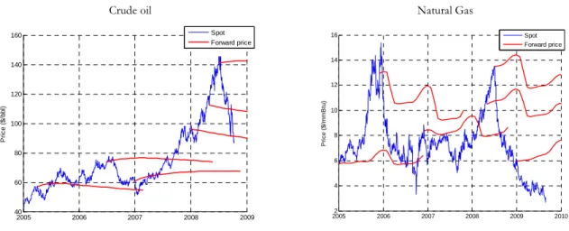
In Figure 1 we present the spot price of different commodities over recent time periods. In many markets, such as crude oil, this spot price is understood to be the price of the front-month futures contract with physical delivery. In other markets, such as shipping, the spot price is an index compiled daily using spot fixings from different brokers, on which the financial futures contracts settle.

20050 2006 2007 2008 2009 2010 50 100 150 200 250 300 350 Crude oil Heating oil Natural gas TD3 shipping

Figure 1. Daily spot prices of crude oil, heating oil, natural gas and the TD3 shipping route from January 2005

(14)

14 Forward curves Crude oil 2005 2006 2007 2008 2009 40 60 80 100 120 140 160 P ri c e ( $ /b b l) Spot Forward price Natural Gas 20052 2006 2007 2008 2009 2010 4 6 8 10 12 14 16 P ri c e ( $ /m m B tu ) Spot Forward price

Figure 2. Spot and forward prices of crude oil and natural gas on different dates

Figure 2 presents the forward curves of crude oil and natural gas on different dates. We observe that the level of the forward curves shifts with the spot price and that the curves transition between contango and

backwardation. Furthermore, the forward curves for natural gas have a seasonal pattern embedded in them. Volatility term structure

0 5 10 15 20 30 40 50 60 70 80 90 100 110 120 Time-to-maturity τ (months) V o la ti li ty ( % ) Crude oil Heating oil Natural gas TD3 shipping

Figure 3. Volatility term structure of futures contracts on crude oil, heating oil, natural gas and TD3 shipping

Figure 3 presents the term structure of volatilities for crude oil, heating oil, natural gas and TD3 shipping. This is the historical volatility of the contracts with fixed time to maturity. We observe that for all these commodities, the volatility of near-term contracts is higher than the volatility of contracts further out on the curve, consistently with Samuelson’s (1965) hypothesis. This is an important feature of commodity markets and happens because they are more inelastic in the short run than in the long run. If the tanker market is saturated it is impossible to add new ships within a month, but new ships can be built to accommodate the increasing demand in the next years.

(15)

15 Correlation structure

The forward prices for a given commodity do not move independently. Observing the correlation matrix of contracts with different maturities quantifies the relationship between these movements. Figure 4 presents the correlation matrix for crude oil contracts. The correlation matrix shows a strong correlation between different contracts, with an 84% correlation between the front-month and 60-month contract. However the correlation between the front-month contract and other contracts decays more rapidly than the correlation between the 60-month contract and neighboring contracts.

0 10 20 30 40 50 60 0 20 40 60 0.8 0.85 0.9 0.95 1 τ1 (months) τ2 (months) C o rr e la ti o n

Figure 4. Correlation structure of crude oil futures

Principal components analysis

To get more insight into the structure of the co-movements of the forward prices we can perform a principal components analysis (PCA) of the price series. This consists in finding the eigenvalues and eigenvectors of the covariance matrix. The eigenvalues can be interpreted as the volatilities of each of the factors and the eigenvectors as the weights with which the principal components shock the forward curve.

We present results of a PCA of the crude oil market in Figure 5. As can be seen from these results, the dominant factor is the first factor, which accounts for 96.9% of the variance. This factor is the parallel shift factor, shifting forward prices in the same direction.

The second factor, explaining 2.8% of the variance, affects the slope of the forward curve by shocking the front end and long end of the forward curve with different signs. This accounts for transitions from contango to backwardation. The third factor affects the convexity of the forward curve by shocking the front and long ends positively and the middle of the curve negatively.

(16)

16 1 2 3 4 5 0 10 20 30 40 50 60 Principal component V o la ti lit y ( % ) 0 10 20 30 40 50 60 -1 -0.5 0 0.5 1 1.5 2 Time-to-maturity τ (months) P C w e ig h t u (τ ) PC 1 PC 2 PC 3

Volatility of the first five principal components Principal component weights

Figure 5. Volatilities and weights for the first principal components of the crude oil market

4. Two-factor model of commodity futures

Consider a commodity forward market where we on each date t observe a forward curve F t T( , ) settling on the spot price S t( ) at date T. S t( ) could represent the spot price of some tradable commodity at time t (e.g. a specific grade of crude oil at a specific location), or the daily published value of an index. If a long forward position is entered at date t, it will receive the difference S T( )−F t T( , )at date T.

Absence of arbitrage tells us (Musiela and Rutkowski, 2004) that under the risk-neutral measure, * * [ ( , )( ( ) ( , ))] 0 ( , ) [ ( )] t t E B t T S T F t T F t T E S T − = = (2.1)

where B t T( , )the time t price of the zero coupon bond that is matures at time T. The forward price of S at time t is the expectation of the spot price at time T, under the risk-neutral measure and given the information at time t. In some markets where the spot is storable, such as equities or currencies, there is a tight arbitrage enforcing the relationship between spot and forward prices. In markets where storage is limited, such as crude oil or shipping, the forward price is determined by supply and demand. It is not our goal here to impose a parametric model for the shape of the initial forward curve, which we take as given, but to give a model of its future stochastic evolution.

Following Baker, Mayfield and Parsons (1998) and Schwartz and Smith (2000), we suggest a two-factor model for the stochastic evolution of the forward curve. We present this model as a forward curve model rather than a spot price model, considering that the commodity derivative markets are generally more liquid than their physical counterparts, and contain more information to calibrate on than the spot price.

(17)

17

We suggest the following two-factor model for the forward curve under the risk-neutral measure:

( ) ( , ) ( ) ( ) ( , ) T t S S L L S L dF t T e dW t dW t F t T dW dW dt α

σ

ρ

− − = + = (2.2)

This is a four-parameter model and as we will show the parameters can be interpreted as follows:

•

σ

S is the volatility of short-term shocks to the forward curve,

•

σ

L is the volatility of long-term shocks,

•

α

is the mean-reversion speed, quantifying how fast short-term shocks dissipate,

•

ρ

is the correlation between short-term and long-term shocks.

Covariance and correlation

This model implies a covariance matrix between contracts that can be calculated as a function of the parameters • Covariance matrix: 1 2 1 2 1 2 1 2 ( ) ( ) 2 2 1 2 ( , ) ( , ) 1 ( , ) Cov , ( , ) ( , ) ( )( ) (1 ) ( , ) t T t T t S L S L L dF t T dF t T T T dt F t T F t T e α e α

σ

ρσ σ

ρσ

ρ σ

τ τ

− − − −   Σ =     = + + + − = Σ (2.3)

where

τ

k = −Tk t is the time to maturity of the contract

• Futures instantaneous volatility function:

( ) 2 2 2 ( , ) ( T t ) (1 ) ( ) inst t T Se L L inst α

σ

₌

σ

− − ₊

ρσ

_{+ −}

ρ σ

₌

σ τ

(2.4) • Spot volatility: 2 2 2 0 ( S L) (1 ) L

σ

=

σ

+

ρσ

+ −

ρ σ

(2.5)

(18)

18 • Correlation matrix: 1 2 1 2 1 2 1 2 1 2 1 2 1 2 ( ) ( ) 2 2 1/ 2 1/ 2 ( ) 2 2 2 ( ) 2 2 2 ( , ) ( , ) ( , ) ( , ) Corr , ( , ) ( , ) ( , ) ( , ) ( )( ) (1 ) ( ) (1 ) ( ) (1 ) ( t inst inst T t T t S L S L L T t T t S L L S L L dF t T dF t T T T T T F t T F t T t T t T e e e e α α α α

ρ

σ

ρσ σ

ρσ

ρ σ

σ

ρσ

ρ σ

σ

ρσ

ρ σ

ρ

− − − − − − − −   _Σ =  =   + + + − =  ₊ _{+ −}   ₊ _{+ −}      =

τ τ

1, 2) (2.6)

All these quantities depend only on the time-to-maturities

τ

= −T t of the contracts involved, and not on time t.

Implied spot price process

In Appendix 2 we show that the spot price model consistent with this forward curve model is:

1 2 2 log ( ) ( ( ) log ( )) ( ) ( ) ( ) ( ) ( ) S L L d S t t S t dt dW t dW t d t m t dt dW t

α µ

σ

µ

σ

= − + + = + (2.7)

i.e. the spot price is mean-reverting to a stochastic mean. This is equivalent to the Schwartz and Smith (2000) model which can be rewritten as

log t t log t t d S S dt dz dz d dt dz ξ χ χ ξ ξ ξ ξ ξ

µ

κ

ξ

σ

κ

ξ µ

σ

  =  + −  + +   = + (2.8)

From equation (2.7) we can see that

α

can be interpreted as the speed of mean-reversion and

σ

L as the volatility of the long-term shocks.

5. Principal components analysis

As discussed in Sclavounos and Ellefsen (2009), futures markets can be analyzed and modeled in a non-parametric way through principal components analysis (PCA) of the covariance matrix, leading to a multi-factor Heath-Jarrow-Morton model of the form

1 ( , ) ( , ) , ( , ) d k k k l kl k dF t T t T dW dW dW dt F t T =

σ

δ

=

∑

= (2.9)

Given the parametric model presented here, we can perform a PCA of the model’s covariance matrix and deduce the shape of its principal components. This will allow us to reformulate the model in terms of independent factors that can be interpreted in terms of their actions on the forward curve.

(19)

19

In the continuous setting we perform the Karhunen-Loève decomposition of the process following Basilevsky (1994). Let f t( , )

τ

=F t t( , +

τ

) be the constant-maturity forward with time-to-maturity

τ

. We want to decompose its evolution into:

1 ( , ) ( , ) ( ) ( , ) k k k k df t t dt u dz f t

τ

_{µ τ}

_λ

_τ

τ

∞ = = +

∑

(2.10) Where:

• The z_k are independent Brownian motions

• The functions ukare the eigenvectors of the covariance matrix Σ( ,

τ τ

1 2) with associated eigenvalues k

λ

: for some arbitrary maximal tenor

τ

_max,

max max 1 2 2 2 1 0 2 0 ( , ) ( ) ( ) ( ) 1 k k k k u d u u d τ τ

τ τ

λ

τ

τ τ

Σ = =

∫

(2.11)

We solve this eigenvector problem analytically in Appendix 3, and show that there are only two distinct functions u_k (because it is a two-factor model), and they can be written in the form

( )

k k k

u

τ

= A e−ατ +B (2.12)

where (A B_k, _k)and

λ

_k are solutions of the two-dimensional eigenvalue problem

max max 2 2 2 max max 2 2 2 2 2 2 2 0 0 2 2 2 2 0 0 ( ) ( ) ( ) ( ) S S L S S L k k k k k S L L S L L e e d e d A A B B e e d e d τ τ ατ ατ ατ τ τ ατ ατ ατ

σ

ρσ σ

τ

σ

ρσ σ

τ

λ

ρσ σ

σ

τ

ρσ σ

σ

τ

− − − − − −   + +     _ _  =   _ _    _ _  + +    

∫

(2.13)

The volatility of factor k is then related to

λ

_k by

σ

_k =

λ

_k . The shape of the eigenfunctions is given in

Figure 6 in the case of crude oil futures. We can notice that u₁ corresponds to parallel shifts of the forward curve, whereas u₂ corresponds to tilts. This is consistent with the two first factors observed doing a PCA of the historical covariance matrix (Sclavounos and Ellefsen, 2009).

(20)

20 0 10 20 30 40 50 60 -0.5 0 0.5 1 1.5 TTM (m) u₁(τ) u₂(τ)

Figure 6. Shape of the eigenfunctions u1( )

τ

and u2( )

τ

for

σ

S =18.1%,

σ

L =23.3%, 1

0.842 yr

α

₌ −

,

ρ

=0.195 and

τ

_max =5 years

This allows us to reformulate the evolution of the individual forward contract expiring at date T, in the risk-neutral measure: 1 1 1 2 2 2 ( , ) ( ) ( ) ( ) ( ) ( , ) dF t T u T t dz t u T t dz t F t T =

σ

− +

σ

− (2.14)

Constant-maturity forward curve

In Appendix 4 we show how this translates to the evolution of constant-maturity forward curve. We show that the constant-maturity futures price f t( , )

τ

=F t t( , +

τ

) can be written as:

1 2 1 2 1 1 2 2 log ( , )f t

τ

=logF(0,t+ +

τ ψ τ ψ

) ( , )t + ( , )t

τ

+g t( )+g t( )+u( ) ( )

τ

f t +u ( )

τ

f t( ) (2.15) where: 2 2 ( ) ( ) ( ) ( ) ( ) 1 ( , ) ( ) 2 k k k k k k k k k k k k df t f t dt dW t dg t B f t dt d t u t dt

α

σ

α

ψ

τ

σ

τ

= − + = = − + (2.16)

Thereby we have decomposed the forward curve’s shape at time t into

• Its initial shape F(0,t+

τ

), which under the risk-neutral measure is also its expected shape

• A deterministic risk-neutral drift

ψ τ ψ

1( , )t + 2( , )t

τ

ensuring that *

[ ( , )] (0, )

t

(21)

21

• A stochastic drift g t₁( )+g t₂( ), independent of the maturity

τ

• Two independent mean-reverting factors f t₁( ) and f t₂( ) (volatilities

σ

_k and mean-reversion speeds

α

_k), giving rise to a parallel shift and a tilt, according to the shape of the factor weights

( )

k u

τ

The spot price process S t( ) is given by the zero time-to-maturity price f t( , 0).

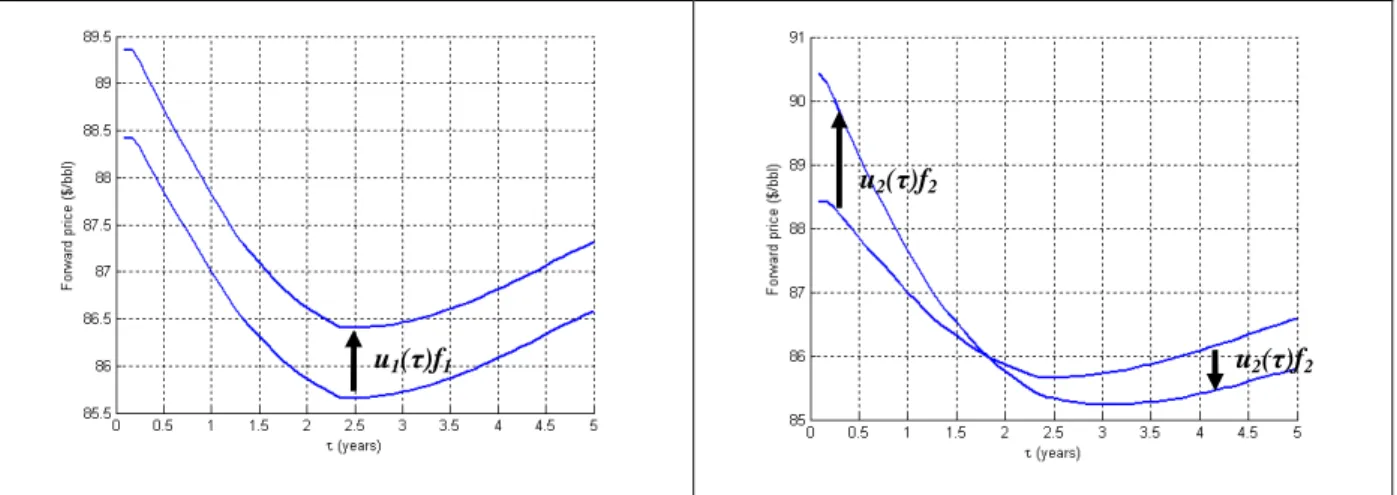
This allows us to express the evolution of the forward curve as the result of shocks from two independent mean-reverting factor values. f₁, the parallel shift factor, affects the average level of the forward curve and is the dominant factor. f₂, the tilt factor, affects the slope of the forward curve, as seen in Figure 7.

Figure 7. Effect of a positive parallel shift (left) and tilt (right) on the forward curve

6. Forward curve seasonality

A number of commodities have seasonal prices. It appears because demand or supply is seasonal, and inventories are not sufficient to smooth this seasonality out over the year. Examples of seasonal commodities are heating oil and natural gas (winter heating demand), gasoline (summer driving season and different volatility requirements during summer and winter) and agricultural products (seasonal supply). This seasonality in spot prices is reflected in the forward prices because of market expectations.

The difficulty when analyzing such forward prices is that the seasonality masks the underlying shifts in level and tilt that we are interested in. When considering such a seasonal commodity, the forward curve can be decomposed into a trend component and a seasonal component:

logF t T( , )=logF t T_T( , ) log+ F t T_S( , ) (2.17) u1(τ)f1

u2(τ)f2

(22)

22

The trend component F t T_T( , ) represents the underlying non-seasonal forward curve, whereas the seasonal component F t TS( , ), which for a given t is 1-year-periodic in T, represents the seasonal aspects of the curve.

Pilipovic (2007) suggests a functional form that we have successfully applied to the natural gas and heating oil markets. In Section 2.10 we will show that this form is also consistent with the static shape of our three-factor model. For the trend component,

3 3

1( ) 2( ) 2 ( ) ( )

1 1 1 2 2 2 3 3 3 3

logF t T_T( , )=(A e−α T t− +B f) +(A e−α T t− +B )f +(A e−α T t− +B e−α T t− +C )f (2.18) This functional form is flexible enough to reproduce the shapes of the underlying forward curve. For the seasonal component, we use sinusoidal seasonality with two harmonics (time must be measured in years)

1 1 2 2

logF t TS( , )=a cos(2 (

π

T−t))+bsin(2 (

π

T−t))+a cos(4 (

π

T−t))+b sin(4 (

π

T−t)) (2.19) The only test of this model is how good the fit to the forward curve is. We find the parameters by least-squares minimization for each day in the data set.

A selection of forward curves is presented in Figure 8. While the fit is not perfect, the trend component seems to correctly capture the underlying trend, and that is what we are ultimately interested in. We then use this trend as the new forward curve, and carry out the rest of the calibration procedure on it.

0 10 20 30 40 50 60 4.5 5 5.5 6 6.5 7 Forward curve Fitted curve Trend component May 21, 2004 0 10 20 30 40 50 60 6.5 7 7.5 8 8.5 9 9.5 Forward curve Fitted curve Trend component May 15, 2008

(23)

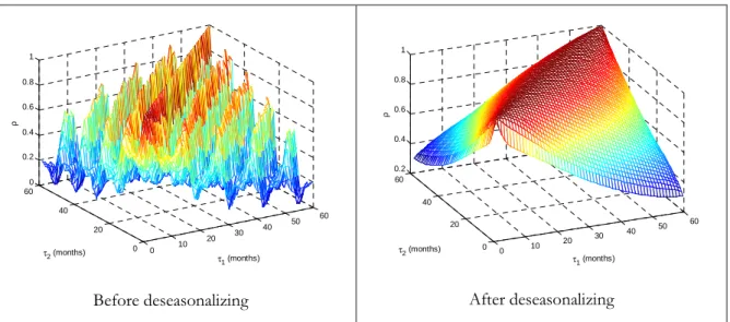
23 0 10 20 30 40 50 60 0 20 40 60 0 0.2 0.4 0.6 0.8 1 τ1 (months) τ2 (months) ρ Before deseasonalizing 0 10 20 30 40 50 60 0 20 40 60 0.2 0.4 0.6 0.8 1 τ1 (months) τ2 (months) ρ After deseasonalizing

Figure 9. Correlation surfaces of Natural Gas futures before and after deseasonalizing the curves

Figure 9 shows the effect of the procedure on the correlation surface. The results of calibrating the two-factor model to this new correlation surface are discussed below.

7. Market calibration

To be successful the model needs to correctly reproduce the volatilities and instantaneous correlations of the traded instruments. We show that there is a good fit to the crude oil, tanker shipping, natural gas and heating oil markets.

Method 1: Least squares fit of the covariance matrix In order to calibrate the model, we perform the following steps:

1. If the forward curve is seasonal (such as natural gas, gasoline, heating oil), deseasonalize it using the technique described above (Section 2.6), and keep only the non-seasonal part F t TT( , j)

2. From the available set of contract prices F t T( , _j), construct constant-maturity prices f t( ,

τ

_j) by linear interpolation using

1 1 1 1 ( ) log ( , ) ( ) log ( , ) log ( , j) j j j j j j , j j j j j t T F t T T t F t T f t T t T T T

τ

+ +

τ

+ + + − + − − = < + < − (2.20)

3. From observations of f t( ,

τ

j) at dates t1,...,tM+1, construct logarithmic returns net of roll yield and their mean value

(24)

24 1 1 1 1 ( , ) log ( , ) 1 ( , ) log ( ) , ( ) ( , ) ( , ) M i j i j i j i i j i j i i j f t f t R t t t R R t f t M

τ

− − = −   _∂ = _ _− − = ∂  

∑

(2.21)

4. Calculate the historical covariance matrix

1 1 ( , ) ( ( , ) ( ))( ( , ) ( )) M j k i j j i k k i R t R R t R M

τ τ

τ

= Σɶ =

∑

− − _(2.22)

5. Find the parameters

σ σ α ρ

S, L, , that minimize the squared error: 2 , , , , , , , 1 min ( , ) ( , ) S L S L N j k j k j k σ σ α ρ σ σ α ρ

∑

₌ Σ

τ τ

− Σɶ

τ τ

 (2.23)

The results are presented in Table 1 for the crude oil, shipping, natural gas and heating oil markets. The results indicate that a satisfactory fit to the volatility term structure and correlation surface can be obtained using the two-factor model presented here. The best calibration results are obtained for crude oil futures, which is arguably the most liquid market of the four. It is also interesting to note the differences between the values obtained. The short-term volatility of shipping futures is extremely high, at 143%, reflecting the high spot price volatility, but its long-term volatility is comparable to the other markets, at 28.7%.

(25)

25

Table 1. Calibration results for different commodity markets

Crude oil (Nymex WTI) Tanker shipping (Imarex TD3)

D

a

ta

Period: April 2005 – October 2008 Contracts: NYMEX WTI futures Frequency: daily

Source: Thomson Datastream

Period: January 2005 – March 2009 Contracts: Imarex TD3 futures Frequency: weekly Source: Imarex P ar am et er s σS σL α ρ 18.1% 23.3% 0.842 0.195 σS σL α ρ 143% 28.7% 3.32 -0.01 V o la ti li ty 0 10 20 30 40 50 60 23 24 25 26 27 28 29 30 31 32 33 TTM (m) V o l (% a n n u a l) Historical Model

Volatility term structure of crude oil futures

0 2 4 6 8 10 12 20 40 60 80 100 120 TTM (m) V o l (% a n n u a l) Historical Model

Volatility term structure of TD3 futures

C o rr el at io n 0 10 20 30 40 50 60 0 20 40 60 0.8 0.85 0.9 0.95 1 τk (m) τl (m) Historical Model

Correlation surface of crude oil futures

0 2 4 6 8 10 12 0 5 10 15 0.4 0.5 0.6 0.7 0.8 0.9 1 τk (m) τl (m) Historical Model

(26)

26 P ri n ci p a l C o m p o n en ts 0 10 20 30 40 50 60 -0.5 0 0.5 1 1.5 TTM (m) u₁(τ) u₂(τ)

Model principal components for crude oil

0 2 4 6 8 10 12 -1.5 -1 -0.5 0 0.5 1 1.5 2 2.5 TTM (m) u₁(τ) u₂(_τ)

Model principal components for TD3 futures

Natural Gas (Nymex Henry Hub) Heating oil (Nymex New York Harbor)

D

a

ta

Period: October 2002 – August 2009 Contracts: NYMEX NG futures Frequency: daily

Source: Reuters

Period: May 2002 – August 2009 Contracts: NYMEX HO futures Frequency: daily Source: Reuters P ar am et er s σS σL α ρ 53% 17.3% 0.762 -0.172 σS σL α ρ 27.6% 26.4% 1.386 0.228 V o la ti li ty 0 10 20 30 40 50 60 15 20 25 30 35 40 45 50 55 60 65 TTM (m) V o l (% a n n u a l) Historical Model

Volatility term structure of natural gas futures

0 2 4 6 8 10 12 14 16 18 26 28 30 32 34 36 38 40 TTM (m) V o l (% a n n u a l) Historical Model

(27)

27 C o rr el at io n 0 10 20 30 40 50 60 0 20 40 60 0.2 0.4 0.6 0.8 1 τk (m) τl (m) Historical Model

Correlation surface of natural gas futures

0 5 10 15 20 0 10 20 0.86 0.88 0.9 0.92 0.94 0.96 0.98 1 τk (m) τl (m) Historical Model

Correlation surface of heating oil futures

P ri n ci p a l C o m p o n en ts 0 10 20 30 40 50 60 -0.6 -0.4 -0.2 0 0.2 0.4 0.6 0.8 1 TTM (m) u₁(τ) u₂(τ)

Model principal components for natural gas

0 2 4 6 8 10 12 14 16 18 -1.5 -1 -0.5 0 0.5 1 1.5 2 TTM (m) u₁(τ) u 2(τ)

(28)

28 Method 2: Calibration of the individual factors

The first two principal components have a simple expression in this model, and can be used for calibration. The method is the same as above, but we replace steps 4 and 5 with:

4’. Calculate the PCA of the historical covariance matrix and extract the first two factor loadings uɶ₁( )

τ

j ,

2( )j

uɶ

τ

5’. Calibrate the exponential functional form on each of the factors by least squares: 2 , , 1 min ( ) ( k j ) k k k N k j k k A B j u A e α τ B α

τ

− =  ₋ ₊   

∑

ɶ (2.24)

We present the results of this method for crude oil futures in Table 2 and Figure 10.

Table 2. Principal component parameters for crude oil futures, using two calibration methods

Principal Component 1 Principal Component 2

Method 1 Method 2 Method 1 Method 2

σ 54.91 % 54.91 % 9.53 % 9.50 % A 0.1218 0.1205 1.7639 1.7385 B 0.4177 0.4189 -0.4435 -0.5148 α 0.8422 0.8713 0.8422 0.6707 0 10 20 30 40 50 60 0.4 0.42 0.44 0.46 0.48 0.5 0.52 0.54 TTM (m) Historical Method 1 Method 2 0 10 20 30 40 50 60 -0.6 -0.4 -0.2 0 0.2 0.4 0.6 0.8 1 1.2 1.4 TTM (m) Historical Method 1 Method 2

Principal Component 1 Principal Component 2

Figure 10. Fit of the shape of the two principal components using the two different calibration methods

(29)

29

We see that the two methods give very close results, except that the second method allows for a different value of

α

which gives a slightly better fit to the second principal component. It should be noted that Method 2 adds one extra free parameter by allowing

α

1 and

α

2 to be different.

8. Forward risk premia – from the risk neutral to the objective measure

The present model has been formulated under the risk-neutral measure. The prices evolve under the real measure. The change of measure from the neutral to the real measure involves introducing a risk-premium

λ

_k for each of the Brownian motions W_k. We assume this risk premium to be constant.

k k k

dW →dW +

λ

dt (2.25)

This will affect the factor processes f t_k( ) and g t_k( ) studied in Section 2.5:

( ) 0 ( ) 0 ( ) ( ( ) ) ( ) ( ) ( )( ( ) ) ( ) ( ) ( ) ( ) ( ) k k t t s k k k k t t s k k k k k k k k k k k k k k k k k k k k k f t e dW s ds df t dW t dt e dW s ds df t f dt dW t f dt dW t α α

σ

λ

σ

σ λ

σ

α

λ

σ λ α

σ

µ α

σ

− − − − = + = + + − + = − + = − +

∫

(2.26)

And for the drift process g tk( ):

( ) 0 ( ) 0 ( ) (1 )( ( ) ) ( ) ( ) ( ) ( ) ( ( ) ) ( ) ( ) k k t t s k k k k k t t s k k k k k k k k k k k k k k g t B e dW s ds dg t B dW t dt dW t dt e dW s ds dt dg t B f t dt α α

σ

λ

σ

λ

α

λ

α

− − − − = − +    =  + − + + − +       =

∫

(2.27)

Hence the factor process f tk( ) follows an Ornstein-Uhlenbeck process mean-reverting to

µ σ λ α

k = k k/ k instead of 0. The definition of g t( ) does not change. We let

µ σ λ

k = k k be the drift term for the factor k. The stochastic evolution of the forward price with tenor T can then be written as

1 1 2 2 1 1 1 2 2 2 ( , ) ( ( ) ( )) ( ) ( ) ( , ) dF t T u T t u T t dt u T t dW u T t dW F t T =

µ

− +

µ

− +

σ

− +

σ

− (2.28)

These results show how to incorporate drifts of the forward curve into the model. These can be based on historical evidence of drifts in prices or subjective evaluations of the expected future prices. This allows

(30)

30

valuation models of physical assets to take into account forecasts of future price evolution. Financial derivatives, however, will be valued under the risk-neutral measure.

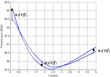
9. Extension to three factors

The model we have considered is sufficient to reproduce the volatility and correlation term structures of most forward markets. However, it only allows for certain movements of the forward curve, i.e. parallel shifts and tilts. As shown previously in the Principal Components Analysis, the forward curve does have other movements, and the third principal component is generally understood to correspond to changes in curvature. Certain strategies, such as a butterfly trade, are especially sensible to this kind of change.

We suggest modeling the third principal component as 2 ( )

u

τ

=Ae−ατ +Be−ατ +C (2.29)

As is shown in Figure 11 it gives a good fit to the third principal component calculated from a historical covariance matrix. With parameters Aand Cpositive and B negative the function u( )

τ

will take positive values for small times-to-maturity, negative values for intermediate

τ

, and then positive values again, thereby affecting the convexity of the curve.

(31)

31

Figure 12. Effect on the forward curve of a positive shock from the third principal component In order to study its interpretation we will consider its effect on the constant-maturity forward curve, as we did in Section 2.4 for the first two components. In Appendix 5 we show that the constant-maturity forward curve can be written as

3 2 1 3 3 3 3 3 3 3 log ( , ) log (0, ) ( ( , ) ( ) ( ) ( )) ( , ) ( ) ( ) ( ) ( ) k k k k k f t F t t g t u f t t B e α τg t C h t u f t

τ

ψ

τ

ψ

τ

= − = + + + + + + + +

∑

(2.30) where 3 3 3 3 3 3 ( ) 3 3 3 3 3 3 3 0 3 3 3 3 3 0 ( ) 2 ( ) ( ) (Ornstein-Uhlenbeck process) ( ) ( ( ) ( )) ( ) ( ) ( ) 2 ( ) ( ) 2 ( ) t t s t df t f t dW t dg t f t g t dt g t e f s ds dh t f t dt h t f s ds α

α

σ

α

− − = − + = − = = =

∫

(2.31)

The process f t₃( ) is an Ornstein-Uhlenbeck process mean-reverting to zero with mean-reversion speed 3

2

α

and volatility

σ

₃. The processes g t₃( ) and h t₃( ) are stochastic drifts – integrals of f t₃( ) with different weights.

10. Model of the static forward curve

While the starting point of our modeling is that the initial forward curve F(0, )T is given, there are situations where one would want to model this curve with a small number of parameters. Using the factor

u3(τ)f3

(32)

32

model presented in this part, we can express the possible shapes of the curve when starting from an initial forward curve: 1 log ( , ) log (0, ) ( , ) ( ) ( ) ( ) N k k k k k f t

τ

F t

τ

ψ

t

τ

g t u

τ

f t = = + +

∑

+ + (2.32)

If we assume the initial forward curve to be flat, F(0, )

τ

=F, this formulation simplifies to:

1 log ( , ) ( ) ( , ) ( ) ( ) N k k k k f t

τ

A t

ψ

t

τ

u

τ

f t = = +

∑

+ (2.33)

Where A t( ) is a time-dependent scalar not depending on time-to-maturity

τ

and 2 0 1 ( , ) ( , ) 2 t k t k s t ds

ψ

τ

= −

_∫

σ

+

τ

(2.34)

This gives the possible shapes that can be taken by the forward curve given an initially flat curve. We can further simplify this by remarking that the first factor, the parallel shift factor, has a function u1( )

τ

that is almost constant, such that the constant term can be merged into the first factor value. Thereby the forward curve can be written as

1 ( , ) exp ( , ) ( ) ( ) N k k k k f t

τ

ψ

t

τ

u

τ

f t =   =  +  

∑

 (2.35)

Hence it can be described by N+1state variables: t f, ₁,..., f_N. Their initial values can be calibrated on the initial forward curve by calculating

(

)

max 0 (0) ( ) log (0, ) k k f u F d τ

τ

τ τ

=

_∫

(2.36)

This formulation also allows us to relate the average level of the forward curve and the first factor value by forming the geometric average weighted by u₁( )

τ

:

max max 1 0 1 0 ( ) ( ) exp ( ) log ( , ) , ( ) ( ) u F t w f t d w u d τ τ

τ

τ τ

τ

τ τ

  = _ _ = 

∫



_∫

(2.37)

(33)

33 such that max max 1 1 1 0 1 0 ( ) ( ) ( , ) ( ) exp ( ) N k k f u t d F t u d τ τ

τ

τ ψ

τ τ

=   +     = _ _      

∑ ∫

∫

(2.38)

We can also examine the initial slope of the curve, that we will use to determine if the curve is in backwardation or contango: 0 0 log ( , 0) f f f t τ τ

τ

=

τ

= ∂ ₌ ∂ ∂ ∂ (2.39) and 1 log ( ) N k k k k u f f t

ψ

τ

=

τ

∂ ∂ ∂ ₌ ₊ ∂

∑

∂ ∂ (2.40)

If we are considering a two-factor model, the first factor is almost flat such that its derivative is zero. In that case the only contribution comes from the second factor:

2 2 2 log ( ) u f f t

ψ

τ

∂ ∂ ∂ ₌ ₊ ∂ ∂ ∂ (2.41)

such that the initial slope of the forward curve is

2 2 2 0 0 0 ( , 0) u ( ) f f t f t τ τ τ

ψ

τ

=

τ

=

τ

= _∂ _∂  ∂ ₌ ₊   ∂  ∂ ∂  (2.42)

Thus the value of f t₂( ) determines the slope of the forward curve.

11. Applications of the market model

Derivatives pricing

The main application of stochastic models of forward curves is in derivatives pricing. The stochastic model that we have derived and calibrated allows for simple pricing of paper derivatives depending on the volatility of prices, such as European or Asian options written on the forward or spot price. In Part 3 we will derive analytical prices of commodity Asian options using the two-factor model derived here.

(34)

34 Real asset valuation and operation

There are a number of physical assets whose value depends on commodity prices and forward curves. Oil or gas reservoirs are a simple example, but more complex assets such as refineries, power plants or oil in transit depend on these prices in a more complex way. Their value depends not only on the spot price but on the complete forward curve, and operational decisions should be made taking into account the possible future evolutions of the complete curve.

The value of such an asset can be written as V t f( , ( ))

τ

where f( )

τ

is the current forward curve. If a two-factor model such as the one in this thesis is adopted, f( )

τ

is a function of the initial forward curve F₀( )

τ

, time t and the factor values f1 and f2, such that the value can be written

1 2

( , ( )) ( , , )

V t f

τ

=V t f f (2.43)

The stochastic evolution of this value function can then be derived, using Ito’s formula and the independence of the factors, as 2 2 2 2 1 2 2 1 2 2 1 2 1 2 2 2 2 2 1 1 1 2 2 2 1 2 2 2 1 1 2 2 1 2 1 2 1 2 1 1 2 2 1 1 ( ) ( ) 2 2 V V V V V dV dt df df df df t f f f f V V V V V V V f f dt dW dW t µ α f µ α f σ f σ f f σ f σ ∂ ∂ ∂ ∂ ∂ = + + + + ∂ ∂ ∂ ∂ ∂ _∂ _∂ _∂ _∂ _∂  _∂ _∂ =_∂ + − _∂ + − _∂ + _∂ + _∂  + _∂ +_∂   (2.44)

Associated with appropriate boundary conditions this allows for the calculation of the value of the real asset and the hedging of its value using the factors. In Part 4 we present the results of this methodology for a physical crude oil trade involving the shipment and possibly storage of crude oil.

Risk evaluation

Once a portfolio of paper and real assets has been valued, the risk of the portfolio can be evaluated using the market model presented here. We assume that given a forward curve f( )

τ

and a date t the portfolio has a value V t f( , ( ))

τ

. If we assume a two-factor model this value can be re-written as V t f f( , ₁, ₂) and its stochastic evolution as 1 2 1 1 2 2 1 2 ( , , ) V V dV t f f dt dW dW f f

µ

∂

σ

∂

σ

= + + ∂ ∂ (2.45) Thereby 1 2 1 1 2 2 1 2 0 0 0 ( ) ( , ( ), ( )) ( ) ( ) t t t V V V t s f s f s ds dW s dW s f f

µ

∂

σ

∂

σ

= + + ∂ ∂

∫

(2.46)

(35)

35

[ ]

1 2 0 ( ) ( , ( ), ( )) t E V t =

∫

µ

s f s f s ds (2.47)

and its standard deviation

1/ 2 2 2 2 2 1 2 1 2 0 0 Std[ ( )] t t V V V t E ds ds f

σ

f

σ

  __∂ _ __∂ _     =   +   ∂ ∂  _ _ _ _ _ _   

∫

 (2.48)

These values can be calculated if the value of Vas a function of the factors and time is known explicitly. Alternatively Monte Carlo simulation can be used, using the two independent processes f1 and f2, to estimate the complete distribution of V at the horizon time t. This Monte Carlo simulation will only require the simulation of two independent stochastic variables and not of each forward price separately.

This information about the distribution of the portfolio value can be used to evaluate the risk of the position and calculate risk measures such as value-at-risk.

Hedging

As seen above a portfolio that depends on forward prices has, according to the two-factor model, a stochastic evolution that can be written

1 2 1 1 2 2 1 2 1 2 1 1 1 2 2 2 ( , , ) ( , , ) V V dV t f f dt dW dW f f t f f dt dW dW

µ

σ

µ

δ σ

∂ ∂ = + + ∂ ∂ = + + (2.49)

In order to hedge the risk related to factor k the portfolio must be complemented with a position of −

δ

_k in the factor k. In that case the hedged portfolio Vɶhas the stochastic evolution

1 2 ( ( , , ) _k( _k _k _k)) _j _j _j j k dV

µ

t f f

δ µ α

f dt

δ σ

dW ≠ = − − +

∑

ɶ _(2.50)

Such a position in a specific factor can only be established with the traded futures F t T( , _j), j=1,...,N. The future with tenor T has the instantaneous evolution

(

1 1 1 2 2 2

)

( , ) ( , ) ( ) ( )

dF t T =F t T

σ

u T−t dW +

σ

u T−t dW (2.51) Consider a portfolio with w_j contracts F t T( , _j), such that

1 ( , ) ( ) N k j j k j k j dW dV w F t T u T t

σ

dt =   ⋅ = −  

∑

 (2.52)

Commodity market modeling and physical trading strategies

Commodity market modeling and physical trading strategies

by

Per Einar S. Ellefsen

Ingénieur de l’Ecole Polytechnique, 2008

Master of Science in Mechanical Engineering

at the

Massachusetts Institute of Technology

June 2010

Commodity market modeling and physical trading strategies

by

Per Einar S. Ellefsen

Table of Contents

1.

INTRODUCTION

τ

τ

τ

µ

σ

µ

σ

2.

MARKET MODELING

σ

σ

ρ

σ

σ

α

ρ

σ

ρσ σ

ρσ

ρ σ

τ τ

τ

σ

σ

ρσ

ρ σ

σ τ

σ

σ

ρσ

ρ σ

ρ

σ

σ

σ

ρσ σ

ρσ

ρ σ

σ

ρσ

ρ σ

σ

ρσ

ρ σ

ρ

τ τ

τ

α µ

σ

σ

µ

σ

µ

κ

ξ

σ

σ

κ

ξ µ

σ

α

σ

σ

δ

∑

_{µ τ}

_λ

_τ