HAL Id: hal-02886493
https://hal.inria.fr/hal-02886493
Submitted on 1 Jul 2020
HAL is a multi-disciplinary open access
archive for the deposit and dissemination of
sci-entific research documents, whether they are
pub-lished or not. The documents may come from
teaching and research institutions in France or
abroad, or from public or private research centers.
L’archive ouverte pluridisciplinaire HAL, est
destinée au dépôt et à la diffusion de documents
scientifiques de niveau recherche, publiés ou non,
émanant des établissements d’enseignement et de
recherche français ou étrangers, des laboratoires
publics ou privés.
Surfaces
Vincent Despré, Jean-Marc Schlenker, Monique Teillaud
To cite this version:
Vincent Despré, Jean-Marc Schlenker, Monique Teillaud. Flipping Geometric Triangulations on
Hy-perbolic Surfaces. SoCG 2020 - 36th International Symposium on Computational Geometry, 2020,
Zurich, Switzerland. �10.4230/LIPIcs.SoCG.2020.35�. �hal-02886493�
Surfaces
Vincent Despré
Université de Lorraine, CNRS, Inria, LORIA, F-54000 Nancy, France [email protected]
Jean-Marc Schlenker
Department of Mathematics, University of Luxembourg, Luxembourg http://math.uni.lu/schlenker/
Monique Teillaud
Université de Lorraine, CNRS, Inria, LORIA, F-54000 Nancy, France https://members.loria.fr/Monique.Teillaud/
Abstract
We consider geometric triangulations of surfaces, i.e., triangulations whose edges can be realized by disjoint geodesic segments. We prove that the flip graph of geometric triangulations with fixed vertices of a flat torus or a closed hyperbolic surface is connected. We give upper bounds on the number of edge flips that are necessary to transform any geometric triangulation on such a surface into a Delaunay triangulation.
2012 ACM Subject Classification Theory of computation → Computational geometry; Mathematics of computing → Discrete mathematics; Mathematics of computing → Geometric topology
Keywords and phrases Hyperbolic surface, Topology, Delaunay triangulation, Algorithm, Flip graph
Digital Object Identifier 10.4230/LIPIcs.SoCG.2020.35
Funding The authors were partially supported by the grant(s) ANR-17-CE40-0033 of the French Na-tional Research Agency ANR (project SoS) and INTER/ANR/16/11554412/SoS of the Luxembourg National Research fund FNR (https://members.loria.fr/Monique.Teillaud/collab/SoS/).
1
Introduction
We investigate triangulations of two categories of surfaces: flat tori, i.e., surfaces of genus 1 with a locally Euclidean metric, and hyperbolic surfaces, i.e., surfaces of genus at least 2 with a locally hyperbolic metric (these surfaces will be introduced more formally in Section 2.1). Triangulations of surfaces can be considered in a purely topological manner: a triangulation of a surface is a graph whose vertices, edges and faces partition the surface and whose faces have three (non-necessarily distinct) vertices. However, when the surface is equipped with a Euclidean or hyperbolic structure, it is possible to consider geometric triangulations, i.e., triangulations whose edges can be realized as geodesic segments that can only intersect at common endpoints (Definition 2). Note that a geometric triangulation can still have loops and multiple edges, but no contractible loop and no contractible cycle formed of two edges. We will prove that any Delaunay triangulation (Definition 4) of the considered surfaces is geometric (Proposition 8).
The flip graph of triangulations of the Euclidean plane is known to be connected; moreover the number of edge flips that are needed to transform any given triangulation with n vertices in the plane into the Delaunay triangulation has complexity Θ(n2) [14]. We are interested in generalizations on this result to surfaces. Flips in triangulations of surfaces will be defined precisely later (Definition 5), for now we can just think of them as similar to edge flips in
© Vincent Despré, Jean-Marc Schlenker, and Monique Teillaud; licensed under Creative Commons License CC-BY
triangulations of the Euclidean plane. Geodesics only locally minimize the length, so the edges of a geometric triangulation are generally not shortest paths. We will prove that the number of geometric triangulations on a set of points can be infinite, whereas the flip graph of “shortest path” triangulations is small but not connected in most situations [8].
IDefinition 1. Let (M2, h) be either a torus (T2, h) equipped with a Euclidean structure h or a closed oriented surface (S, h) equipped with a hyperbolic structure h. Let V ⊂ M2 be a set of n points. The geometric flip graph FM2,h,V of (M2, h, V ) is the graph whose vertices are the geometric triangulations of (M2, h) with vertex set V and where two vertices are connected by an edge if and only if the corresponding triangulations are related by a flip.
Our results are mainly interesting in the hyperbolic setting, which is richer than the flat setting. However, to help the readers’ intuition, we also present them for flat tori, where they are slightly simpler to prove and might even be considered as folklore. The geometric flip graph is known to be connected for the special case of flat surfaces with conical singularities and triangulations whose vertices are these singularities [19].
The main results of this paper are:
The geometric flip graph of (M2, h, V ) is connected (Theorems 12 and 14).
The Delaunay triangulation can be reached from any geometric triangulation by a path in the geometric flip graph FM2,h,V whose length is bounded by n2 times a quantity
measuring the quality of the input triangulation (Theorems 16 and 19).
If an initial triangulation of the surface only having one vertex is given, then the Delaunay triangulation can thus be computed incrementally by inserting points one by one in a very standard way: for each new point, the triangle containing it is split into three, then the Delaunay property is restored by propagating flips. This approach, based on flips, can handle triangulations of a surface with loops and multiarcs, which is not the case for the approach based on Bowyer’s incremental algorithm [6, 5].
2
Background and notation
2.1
Surfaces
In this section, we first recall a few notions, then we illustrate them for the two classes of surfaces (flat tori and hyperbolic surfaces) that we are interested in.
Let M2 be a closed oriented surface, i.e., a compact connected oriented 2-manifold
without boundary. There is a unique simply connected surface gM2, called the universal cover
of M2, equipped with a projection ρ : gM2→ M2 that is a local diffeomorphism. There is
a natural action on gM2 of the fundamental group π1(M2) of M2 so that for all p ∈ M2, ρ−1(p) is an orbit under the action of π1(M2). We will denote asp a lift of p, i.e., one ofe
the elements of the orbit ρ−1(p). A fundamental domain in gM
2 for the action of π1(M2)
on gM2 is a connected subset Ω of gM2 that intersects each orbit in exactly one point, or,
equivalently, such that the restriction of ρ to Ω is a bijection from Ω to M2[17]. The genus g
of M2 is its number of handles. In this paper, we consider surfaces with constant curvature
(0 or −1). The value of the curvature is given by the Gauss-Bonnet Theorem and thus only depends on the genus: a surface of genus 0 only admits spherical structures (not considered here); a flat torus is a surface of genus 1 and admits Euclidean structures; a surface of genus 2 and above admits only hyperbolic structures (see below).
Flat tori
We denote by T2
the topological torus, that is, the product T2
= S1× S1 of two copies
of the circle. Flat tori are obtained by taking the quotient of the Euclidean plane by an Abelian group generated by two independent translations. There are in fact many different Euclidean structures on T2; if one considers Euclidean structures up to homothety – which is sufficient for our purposes here – a Euclidean structure is uniquely determined by a vector
u in the upper half-plane R × R>0: to such a vector u is associated the Euclidean structure
(T2, h
u) ∼ R2/(Ze1+ Zu) , where e1= (1, 0) and u = (ux, uy) ∈ R2 is linearly independent
from e1. The orbit of a point of the plane is a lattice. The area Ah of the surface is |uy|.
The plane R2, equipped with the Euclidean metric, is then isometric to the universal cover of the corresponding quotient surface.
Hyperbolic surfaces
We now consider a closed oriented surface S (a compact oriented surface without boundary) of genus g ≥ 2. Such a surface does not admit any Euclidean structure, but it admits many
hyperbolic structures, corresponding to metrics of constant curvature −1, locally modeled on
the hyperbolic plane H2. Given a hyperbolic structure h on S, the surface (S, h) is isometric
to the quotient H2/G, where G is a (non-Abelian) discrete subgroup of the isometry group P SL(2, R) of H2 isomorphic to the fundamental group π
1(S). The universal cover eS is
isometric to the hyperbolic plane H2.
2.2
The Poincaré disk model of the hyperbolic plane
In the Poincaré disk model [1], the hyperbolic plane is represented as the open unit disk D2 of R2
. The geodesic lines consist of circular arcs contained in the disk D2 and that are
orthogonal to its boundary (Figure 1 (left)). The model is conformal, i.e., the Euclidean angles measured in the plane are equal to the hyperbolic angles.
We won’t need the exact expression of the hyperbolic metric here. However, the notion of a hyperbolic circle is relevant to us. Three non-collinear points in the hyperbolic plane H2 determine a circle, which is the restriction to the Poincaré disk of a Euclidean circle or line. If C is a Euclidean circle or line and φ : D2 → D2 is an isometry of the hyperbolic plane,
then φ(C ∩ D2
) is still the intersection with D2 of a Euclidean circle or a line.
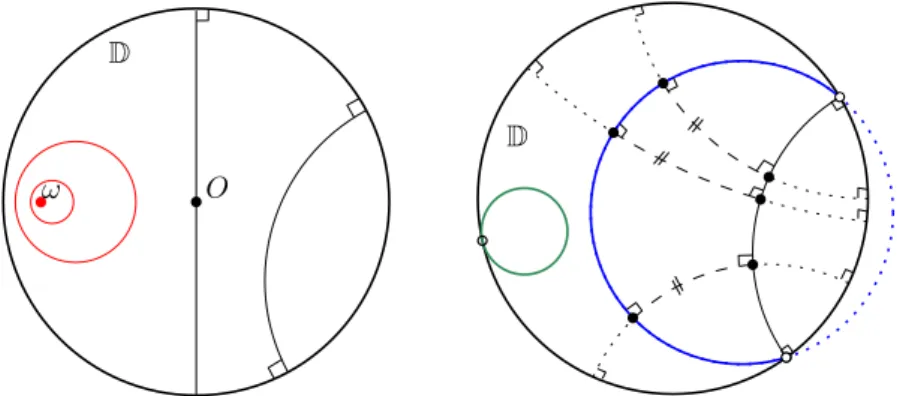
A key difference with the Euclidean case is that the “circle” defined by 3 non-collinear points in H2 is generally not compact (i.e., it is not included in the Poincaré disk). The compact circles are sets of points at constant (hyperbolic) distance from a point. Non-compact circles are either hypercycles, i.e., connected components of the set of points at constant (hyperbolic) distance from a hyperbolic line, or horocycles (Figure 1 (right)) [13].1
Therefore, the relatively elementary tools that can be used for flat tori must be refined for hyperbolic surfaces. Still, some basic properties of circles still hold for non-compact circles. A non-compact circle splits the hyperbolic plane into two connected regions; we will call a
disk the region of the Poincaré disk that is convex, in the hyperbolic sense (Figure 2).
Triangulations of hyperbolic spaces have been studied [3] and implemented in cgal in 2D [4]. Note that that previous work was not considering non-compact circles as circles.
1
D O
ω D
Figure 1 The Poincaré disk. Left: Geodesic lines (black) and compact circles (red) centered at
point ω. Right: A horocycle (green). A hypercycle (blue), whose points have constant distance from the black geodesic line.
D D
Figure 2 Shaded: Two (convex) non-compact disks.
2.3
Triangulations on surfaces
Let (M2, h) be either a torus (T2, h) equipped with a Euclidean structure h or a closed
surface (S, h) equipped with a hyperbolic structure h.
For a given finite set of points V ⊂ M2, we will consider any two topological triangulations T and T0 of M2 with vertex set V as equivalent if for any two vertices u and v in V , the
edges of T with vertices u and v are in one-to-one correspondence with the edges of T0 with the same vertices u and v through homotopies with fixed points.
Recall that given two distinct points v, w ∈ M2, any homotopy class of paths on M2with
endpoints v and w contains a unique geodesic segment [10, Chapter 1]. So, any triangulation is equivalent to a unique geodesic triangulation, i.e., a triangulation whose edges are geodesic segments. Note that the edges of a geodesic triangulation can intersect in their interiors.
IDefinition 2. A triangulation T on M2 is said to be geometric for h if the edges of its equivalent geodesic triangulation do not intersect except at common endpoints.
If T is a triangulation of M2, its inverse image ρ−1(T ) is the (infinite) triangulation of
g
M2whose vertices, edges and faces are the lifted images by ρ−1 of those of T .
IDefinition 3. The diameter ∆(T ) of a geodesic T is the smallest diameter of a fundamental
The diameter ∆(T ) is not smaller than the diameter of (S, h). It is unclear how to compute ∆(T ) algorithmically and the problem looks difficult. However bounds are easy to obtain: ∆(T ) is at least equal to the maximum of the diameters of the triangles of ρ−1(T ) in gM2
and is at most the sum of the diameters of these triangles.
IDefinition 4. We say that a triangulation T of M2 is a Delaunay triangulation if for each face f of T and any face ef of ρ−1(T ), the open disk in gM2that is bounded by the circle passing through the three vertices of ef is empty, i.e., it contains no vertex of ρ−1(T ). It follows that if T is a geodesic Delaunay triangulation of M2with vertex set V , then ρ−1(T )
is the Delaunay triangulation in gM2of ρ−1(V ). So, for a non-degenerate set of points on
M2, since the Delaunay triangulation of their lifts in gM2 is unique, there is also a unique
geodesic Delaunay triangulation on M2. However its edges may a priori intersect.
For a degenerate set V of points, at least two adjacent triangles in the possible Delaunay triangulations of ρ−1(V ) in gM2 have cocircular vertices. Any triangulation of the subset
C of ρ−1(V ) consisting of c cocircular points is a Delaunay triangulation. Any of these
triangulations can be transformed in any other by O(c) flips [14]. From now on, we can thus assume that the set of points V on the surfaces that we consider is always non-degenerate.
We will see in Section 3 that any Delaunay triangulation of M2 is in fact geometric.
Remark that, even for a hyperbolic surface, the closure of every empty disk in the universal cover H2is compact. Indeed, any non-compact disk contains at least one disk of
any diameter, so, at least one disk of diameter ∆(T ), thus it contains a fundamental domain (actually, infinitely many fundamental domains) and its interior cannot be empty.
Let us now give a natural definition for flips in triangulations of surfaces.
IDefinition 5. Let T be a geometric triangulation of M2. Let (v1, v2, v3) and (v2, v1, v4) be two adjacent triangles in T , sharing the edge e = (v1, v2). Let us lift the quadrilateral
(v1, v2, v3, v4) to a quadrilateral (ve1,ve2,ve3,ve4) in gM2 so that (ve1,ve2,ve3) and (ve2,ve1,ve4) form
two adjacent triangles of ρ−1(T ) sharing the edge ee = (ve1,ve2).
Flipping e in T consists of replacing the diagonal ee in the quadrilateral (ve1,ve2,ve3,ve4)
(which lies in gM2, i.e., R2 or H2) by the geodesic segment (ve3,ve4), then projecting the two new triangles (ve3,ve4,ve2) and (ve4,ve3,ve1) to M2 by ρ.
We say that the flip of T along e is Delaunay if the triangulation is locally Delaunay in the quadrilateral after the flip, i.e., the disk inscribing (ve3,ve4,ve2) does not contain ve1 (and
the disk inscribing (ve4,ve3,ve1) does not contain ve2).
An edge e is said to be Delaunay flippable if the flip along e is Delaunay.
Note that even though T is geometric in this definition, the triangulation after a flip is not necessarily geometric. We will prove later (Lemma 9) that a Delaunay flip transforms a geometric triangulation into a geometric triangulation.
Triangulations and polyhedral surfaces
The Euclidean plane can be identified with the plane (z = 1) in R3, while the Poincaré model of the hyperbolic plane can be identified with the unit disk in that plane. We can now use the stereographic projection σ : S2\ {s
0} → R2 to send the unit sphere S2 to this plane
(z = 1), where s0= (0, 0, −1) is the pole. In this projection, each point p 6= s0 on the sphere
is sent to the unique intersection with the plane (z = 1) of the line going through s0 and p. The inverse image of the plane (z = 1) is S2\ {s0}, while the inverse image of the disk
containing the Poincaré model of the hyperbolic plane is a disk, which is the set of points of S2 above a horizontal plane.
Let T? be a triangulation of the Euclidean or the hyperbolic plane – for instance, T? could be the inverse image ρ−1(T ) of a triangulation T of a surface (M2, h), in which case T?
has infinitely many vertices. We associate to T?
a polyhedral surface Σ in R3, constructed
as follows. The construction is similar to the classic duality originally presented with a paraboloid in the case of (finite) triangulations in a Euclidean space [9]. It can also be seen as a simpler version, sufficient for our purpose, of the construction presented for triangulations in hyperbolic spaces using the space of spheres [3].
The vertices of Σ are the inverse images on S2 by σ of the vertices of T?.
The edges of Σ are line segments in R3 corresponding to the edges of T? and the faces of
Σ are triangles in R3 corresponding to the faces of T?.
Note that Σ is not necessarily convex. We can make the following well-known remarks. Let
t1 and t2 be two triangles of T? sharing an edge e, and let tΣ1 and tΣ2 be the corresponding
faces of the polyhedral surface Σ, sharing the edge eΣ. Then Σ is concave at eΣif and only
if e is Delaunay flippable. Flipping e in the triangulation T? in the plane corresponds to replacing the two faces tΣ
1 and tΣ2 of Σ by the two other faces of the tetrahedron formed by
their vertices. That tetrahedron lies between Σ and S2. We obtain a new edge eΣ0 at which the new polyhedral surface Σ0 is convex, and which is strictly closer to S2 than Σ. By an
abuse of language, we will say that Σ0 contains Σ, which we will denote as Σ ⊂ Σ0. As a consequence, Σ is convex if and only if T? is Delaunay.
There is a direct corollary of this statement: Given a (non-degenerate, see above) discrete set V of points in R2
or H2, there is a unique Delaunay triangulation with this set of vertices.
However we are going to see in the next two sections that there can be infinitely many geometric (non-Delaunay) triangulations on a surface, with the same given finite vertex set.
3
Geometric triangulations of surfaces
We consider now Dehn twists, which are usually considered as acting on the space of metrics on a surface [7], but are defined here equivalently, for simplicity, as acting on triangulations of a closed oriented surface (M2, h) equipped with a fixed Euclidean or hyperbolic structure
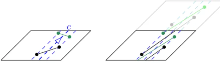
(figures in this section illustrate the flat case, but the results are proved for both flat and hyperbolic cases). Let T be a triangulation of (M2, h), with vertex set V , and let c be
an oriented homotopically non-trivial simple closed curve on M2\ V . We define a new
triangulation τc(T ) of M2 by performing a Dehn twist along c: whenever an edge e of T
intersects c at a point p, we orient e so that the unit vectors of the tangent plane along e and
c form a positively oriented basis (see Figure 3 (left)), and then replace e by the oriented
path following e until p, then following c until it comes back to p, then following e until its endpoint (see Figure 3 (right)). This defines a map τc from the space of triangulations of T2
with vertex set V to itself. Note that, even if T is a geometric triangulation, τc(T ) is not
necessarily geometric. If we denote by −c the curve c with the opposite orientation, then one easily checks that τ−c= τc−1.
ILemma 6. There exists a geometric triangulation T of (M2, h) and a simple closed curve c ⊂ M2 such that for all k ∈ Z, τck(T ) is geometric.
Proof. Let us focus on the hyperbolic case (the construction is easier in the flat case). Consider a pants decomposition of M2and denote as C the set of its boundary curves, which
are simple closed geodesics. Let us choose c in C and ε > 0. We denote by c−, c+ the two
hypercycles at distance ε from c on both sides of c. The value of ε must be sufficiently small so that the region between c− and c+ is an annulus drawn on M2that does not intersect
c
e
p
Figure 3 Transformation of an edge e by the Dehn twist along c on a flat torus T2. Here the black parallelepiped is a fundamental domain, and the gray one, used for the construction of the image of e by τc, is another fundamental domain, image through an element of the the group Γ of
isometries.
any curve in C \ {c}. Each curve in C \ {c} is split into two geodesic segments by putting two points on it; let us add the two segments as edges of T . Let us put two points on c−
(resp. c+) and add as edges of T the two geodesic segments between them, whose union
forms a curve homotopic to c. Each pair of pants not bounded by c, as well as the two “shortened pants” bounded by c− and c+, can be decomposed into two hexagons, which can
easily been triangulated with geodesic edges. All these edges are left unchanged by τc (or
τ−c) as they do not intersect c. The annulus between c− and c+ can be triangulated with
four edges intersecting c exactly once. We realize the image by τc of each of these four edges
as a geodesic segment – there is a unique choice in the homotopy class of the path described above (Figure 4). The annulus is convex, as the projection onto M2 of the intersection of
two (convex) disks (Figure 2), so, the geodesic segment is completely contained in it. Let
c c+ c−
e
Figure 4 Image of e by a Dehn twist (middle), realized as a geodesic edge (right).
e, e0 be two edges of T . If either e or e0 does not intersect c, then their images by τc (or τ−c)
remain disjoint, as they lie in different regions separated by c− and c+. If e and e0 intersect c, then again their images by τc (or τ−c) remain disjoint, as their endpoints appear in the
same order on c− and c+ and two geodesic lines cannot intersect more than once (Figure 5).
As a consequence, τc(T ) and τ−c(T ) are geometric. They are not equivalent as each edge e
c
Figure 5 The Dehn twist of two edges along c for two edges intersecting c.
crossing c is replaced by an edge that does not lie in the same homotopy class as e. The same result follows by induction for τk
c(T ) for any k ∈ Z. J
ICorollary 7. For any closed oriented surface (M2, h), there exists a finite set of points V ⊂ M2 such that the graph of geometric triangulations with vertex set V is infinite.
IProposition 8. Any Delaunay triangulation of a closed oriented surface (M2, h) is geo-metric.
Proof. Let V be a finite set of points on M2, and let T be a Delaunay triangulation of
(M2, h) with vertex set V . Realize every edge of T as a the unique geodesic segment in its
homotopy class, so that T is geodesic. We argue by contradiction and suppose that T is not geometric, so that there are two edges e1and e2that intersect in their interiors. We then lift e1and e2 to edgesee1 andee2of ρ
−1(T ) whose interiors still intersect.
We can find two distincts faces ef1and ef2of ρ−1(T ) such thatee1is an edge of ef1andee2is
an edge of ef2. Let fC1 and fC2be the circles inscribing ef1 and ef2, respectively. Since ρ−1(T )
is Delaunay, fC1 and fC2bound empty disks fD1and fD2, i.e., open disks not containing any
point of ρ−1(V ). Recall that, as mentioned in Section 2.3, the closures of empty disks are compact even in the hyperbolic case, and thatee1⊂ fD1 andee2⊂ fD2 (edges are considered as open). The two circles fC1 and fC2 intersect twice as the intersection point ofee1 andee2
lies in fD1∩ fD2. Let eL be the geodesic line through the intersection points. The endpoints
ofee1 are on fC1\ fD2 and those of ee2 are on fC2\ fD1, so the two pairs of endpoints are on
opposite sides of eL. As a consequence,ee1andee2 are on opposite sides of eL, so they cannot
intersect. This leads to a contradiction. J
4
The flip algorithm
Let us consider a closed oriented surface (M2, h). The flip algorithm consists of performing
Delaunay flips in any order, starting from a given input geometric triangulation of M2, until
there is no more Delaunay flippable edge.
In this section, we first define a data structure that supports this algorithm, then we prove the correctness of the algorithm.
4.1
Data structure
In both cases of a flat or hyperbolic surface, the group of isometries defining the surface is denoted as G. We assume that a fundamental domain Ω0is given. By definition (Section 2.1),
g
M2is the union G(Ω0) of the images of Ω0 under the action of G.
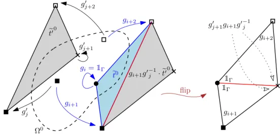
To represent a triangulation on the surface, we propose a data structure generalizing the data structure previously introduced for triangulations of flat orbifolds [6] and triangulations of the Bolza surface [15]. The combinatorics of the triangulation is given by the set of its vertices V on the surface and the set of its triangles, where each triangle gives access to its three vertices in V and its three adjacent triangles, and each vertex gives access to one of its incident triangles. The geometry of the triangulation is given by the set eV0 of the lifts
of its vertices that lie in the fundamental domain Ω0and one liftet
0in gM
2 of each triangle t = (v0,t; v1,t; v2,t) of the triangulation, chosen among the (one, two, or three) lifts of t in gM2
having at least one vertex in Ω0: et0 has at least one of its verticesvfi,t
0
in Ω0 (i = 0, 1, or 2); then the other vertices ofet
0 are images g
i+1,t· ^vi+1,t
0
and gi+2,t· ^vi+2,t
0
of two vertices in eV0, where g
i+1,t and gi+2,t are elements of G (indices are taken modulo 3). In the data
structure, each vertex v on the surface has access to its representativeev0, and each triangle t on the surface has access to the isometries g0,t, g1,t, and g2,t allowing to constructet0, at least one of the isometries being the identity1G. Note that two triangles t and t0 of T that are
adjacent on the surface are represented by two triangleset0and et0
0
, which are not necessarily adjacent in gM2 (Figure 6 (left)). However, there is an isometry g in G such thatet0 and
Let T be an input triangulation given as such a data structure. Figure 6 illustrates a Delaunay flip performed on two adjacent triangles t and t0 on the surface. The triangle e
t00is first moved so that the vertices of the edge to be flipped coincide. Then the edge is
flipped. The isometries in the two triangles created by the flip are easy to compute from the isometries stored in t and t0. Note that the order in which isometries are composed is crucial in the hyperbolic case, as they do not commute. We have shown that the data structure can be maintained through flips.
Ω0 e t0 gi=1Γ gi+1 gi+2 gi+1g0−1j · et0 0 gi+1 gi+2 g0j g0 j+1 g0j+2 1Γ 1Γ gj+10 gi+1g0−1j e t00 flip
Figure 6 A flip. Here (hyperbolic) triangles are represented schematically with straight edges.
Left: the two triangleset 0 and
e
t00 before the flip. Here g
i=1G. Right: the isometries in the two
triangles created by the flip.
4.2
Correctness of the algorithm
The following statement is a key starting point.ILemma 9. Let T be a geometric triangulation of (M2, h), and let T0 be obtained from T by a Delaunay flip. Then T0 is still geometric.
Proof. Let e be a Delaunay flippable edge ande a lift in ge M2. Denote the vertices ofee by ev and ev0. Let
e
t1 andte2 be the triangles of ρ−1(T ) incident toee. To prove that T0 is geometric,
it is sufficient to prove thatte1∪te2 is a strictly convex quadrilateral.
Let fC1 (resp. fC2) be the circle through the three vertices of te1 (resp. te2). Note that
f
C1 and fC2 may be non-compact. Let fD1 and fD2 be the corresponding disks (as defined
in Section 2.2 on case of non-compact circles). The disk fD1 (resp. fD2) is convex (in the
Euclidean plane if M2 is a flat torus, or in the sense of hyperbolic geometry if M2 is a
hyperbolic surface) and containste1 (resp. te2). The fact that e is Delaunay flippable then
implies thatte1andte2are contained in fD1∩ fD2 (see Figure 7). As a consequence, the sum of
angles ofte1andte2at ev is smaller than the interior angle atev of fD1∩ fD2, which is at most
π, and similarly at ev0. As a consequence, the quadrilateral
e
t1∪te2is strictly convex atev and e
v0. Since it is strictly convex at its other two vertices (as each of these vertices is a vertex of
a triangle), it is strictly convex, and the statement follows. J The following lemma, using the diameter of the triangulation (Definition 3), is central in the proof of the termination of the algorithm (Theorem 14) for hyperbolic surfaces and in its analysis for both flat tori and hyperbolic surfaces (Section 5).
e e f D1 f D2 e t1 te2 e v e v0
Figure 7 The quadrilateral is convex (edges are represented schematicaly as straight line segments).
I Lemma 10. Let T be a geometric triangulation of (M2, h). Then, the flip algorithm starting from T will never insert an edge longer than 2∆(T ).
Note that the length of an edge can be measured on any of its lifts in the universal covering space gM2.
Proof. Let Tk be the triangulation obtained from T = T0 after k flips and let Σk be the
corresponding polyhedral surface of R3 as defined in Section 2.3. Since we perform only
Delaunay flips, Σ0⊂ . . . ⊂ Σk⊂ Σk+1(with the abuse of language mentioned in Section 2.3).
We will prove the result by contradiction. Let us assume that Tk has an edge e of length
larger than 2∆(T ). Let Ω be a fundamental domain of M2having diameter ∆(T ), given as
the union of lifts of triangles of T = T0(it is not clear how to compute such a fundamental
domain efficiently but its existence is clear). Let v be the midpoint of e andev its lift in Ω.
Letee = (ve1,ve2) be the unique lift of e whose midpoint isev. The domain Ω is strictly included
in the disk eD of radius ∆(T ) and centered atev, by definition of ∆(T ) (see Figure 8 (left)).
Let PD denote the plane in R3containing the circle on S2that is the boundary of σ−1(D)
(recall that σ denotes the stereographic projection, see Section 2.3), and let p denote the point σ−1(ev) on S2. As p ∈ σ−1(Ω) ⊂ σ−1( eD), the projection pΣ0 of p onto Σ
0 lies above PD (Figure 8 (right)).
Now, denote the edge σ−1(ee) on S2 as (p
1, p2). The points p1and p2lie outside σ−1(D).
So, the corresponding edge eΣ= [p1, p2] of Σk lies below the plane PC, thus the projection
pΣk∈ [p
1, p2] of p onto Σk lies below PC.
From what we have shown, pΣk is a point of Σ
k that lies strictly between the pole s0and
the point pΣ0 of Σ
0, which contradicts the inclusion Σ0⊂ Σk. J
We will now show that, for any order, the flip algorithm terminates and returns the Delaunay triangulation of the surface. The proof given for the hyperbolic case would also work for the flat case. However we propose a more elementary proof for the flat case.
Flat tori
The case of flat tori is easy, and might be considered as folklore. However, as we have not found a reference, we give the details here for completeness.
We define the weight of a triangle t of a geometric triangulation T of T2as the number of vertices of ρ−1(T ) that lie in the open circumdisk of a lift of t. The weight w(T ) of T is defined as the sum of the weights of its triangles.
S2 s0 R2 D ve1 ve2 p1 p2 e D ev pΣk p pΣ0 Ω D e v e v2 e v1 e D Ω e e PD
Figure 8 Illustration for the proof of Lemma 10 (for a hyperbolic surface). Left: notation in H2. Right: contradiction seen in a cutting plane in R3.
ILemma 11. The weight w(T ) of a triangulation T of a flat torus (T2, h) is finite. Let T0 be the triangulation obtained from a geometric triangulation T after performing a Delaunay flip. Then w(T0) ≤ w(T ) − 2.
Proof. The closed circumdisk of any triangle in R2 is compact, so, it can only contain a finite number of vertices of ρ−1(T ). The sum w(T ) of these numbers over triangles of T is clearly finite as the number of triangles of T is finite. Let us now focus on a quadrilateral in R2
that is a lift of the quadrilateral on T2 whose diagonal e is flipped. Let fD
1and fD2
denote the two open circumdisks in R2before the flip and fD0
1 and fD20 denote the two open
circumdisks after the flip, then fD10 ∪ fD02⊂ fD1∪ fD2and fD01∩ fD20 ⊂ fD1∩ fD2 (see Figure 9).
Moreover, by definition of a Delaunay flip, the union fD01∪ fD02 contains at least two fewer
e e f D1 f D2 f D0 1 f D20
Figure 9 CircumdisksDf1andDf2before flippinge ande Df1 andDf20 after the Delaunay flip. vertices of ρ−1(T ) than fD1∪ fD2, which are the two vertices of the quadrilateral that are not
The result follows trivially:
ITheorem 12. Let T be a geometric triangulation of a flat torus with finite vertex set V .
The flip algorithm terminates and outputs the Delaunay triangulation of V . ICorollary 13. The geometric flip graph FT2,h,V is connected.
Hyperbolic surfaces
To show that the flip algorithm terminates in the hyperbolic case, we cannot mimic the proof presented for the flat tori since the circumcircle of a hyperbolic triangle can be non-compact (see Section 2.2) and thus can have an infinite weight. Note also that the proof cannot use a property on the angles of the Delaunay triangulation similar to what holds in the Euclidean case: in H2, the locus of points seeing a segment with a given angle is not a circle arc, and
thus the Delaunay triangulation of a set of points in H2 does not maximize the smallest angle of triangles. The proof relies on Lemma 10.
ITheorem 14. Let T be a geometric triangulation of a closed hyperbolic surface with finite
vertex set V . The flip algorithm terminates and outputs the Delaunay triangulation of V . Proof. We use the same notation as in the proof Lemma 10. Once an edge of Tk is flipped, it
can never reappear in the triangulation, as the corresponding segment in R3becomes interior
to the polyhedral surface Σk+1 (see Section 2.3) and further surfaces Σk0, k0 ≥ k + 1. In
addition, all the introduced edges have length smaller than 2∆(T ) by Lemma 10. Moreover, there is only a finite number of edges with vertices in V that are shorter than 2∆(T ) on
S, as a circle given by a center and a bounded radius is compact. So, the flip algorithm
terminates. The output does not have any Delaunay flippable edge, so, it is the Delaunay
triangulation. J
ICorollary 15. The geometric flip graph FS,h,V is connected.
5
Algorithm analysis
For a triangulation on n vertices in the Euclidean plane, counting the weights of triangulations leads to the optimal O(n2) bound. However the same argument does not yield a bound even
for the flat torus, since points must be counted in the universal cover.
ITheorem 16. For any triangulation T with n vertices of a torus (T2, h), there is a sequence of flips of length Ch· ∆(T )2· n2 connecting T to a Delaunay triangulation of (T2, h), where
Ch only depends on h.
Proof. Let e = (v1, v2) be an edge appearing during the flip algorithm, andve1(resp.ve2) be a
lift of v1(resp. v2), such that (ve1,ve2) is a liftee of e. The pointve2lies in a circle C of diameter 4∆(T ) centered atve1by Lemma 10. Let M be the affine transformation that maps the lattice
of the lifts of v2to the square lattice Z2. M (C) is a convex set and from Pick’s theorem [20],2
the number of points of Z2in M (C) is smaller than area(M (C)) + 1/2 · perimeter(M (C)) + 1,
which is also a bound on the number of possible points ve2 in C and thus the number of
possible edges e. The area of M (C) is 1/Ah· area(C) since det(M ) = 1/Ah, but there is no
simple formula for its perimeter. As already mentioned in the proof of Theorem 14, an edge can never reappear after it was flipped. Moreover, there are n2/2 sets of points {v1, v2} (v1
and v2 may be the same point), which yields the result. J
2
The rest of this section is devoted to computing the number of edges not longer than 2∆(T ) between two fixed points v1 and v2 on a hyperbolic surface (S, h). Counting the
number of points in a disk of fixed radius would give an exponential bound because the area of a circle in H2 is exponential in its radius [16]. Note that we only consider geodesic edges,
so we only need to count homotopy classes of simple paths. The behavior of the number Nl
of simple closed curves smaller than a fixed length l is well understood: Nl/l6g−6 converges
to a positive constant depending “continuously” on the structure h [18]. However, we need a result for geodesic segments instead of geodesic closed curves, and Mirzakhani’s proof is too deep and relies on too sophisticated structures to easily be generalized. So, we will only prove an upper bound on the number of segments. Such an upper bound could be derived from the theory of measured laminations of Thurston, which is also quite intricate. Fortunately, a more comprehensible proof, specific to simple closed geodesic curves on hyperbolic structures, can be found in a book published by the French Mathematical Society [12, 4.III, p.61-67] [11]. While recalling the main steps of the proof, we show how to extend it to geodesic segments. Let Γ = {γi, i = 1, . . . , 3g − 3} be a set of 3g − 3 simple disjoint closed geodesics on (S, h)
not containing v1 and v2 that forms a pants decomposition on S, where each γi belongs to
two different pairs of pants. A set {γi, i = 1, . . . , 3g − 3} of disjoint closed annuli is defined
on S, where each γi is a tubular neighborhood of γi containing none of v1, v2. This yields
a decomposition of S into 3g − 3 annuli γi (i = 1, . . . , 3g − 3) and 2g − 2 pairs of “short
pants” Pj (j = 1, . . . , 2g − 2). For i = 1, . . . , 3g − 3, let us denote as ∂γi any one of the two
curves bounding the annulus γi (this is an abuse of notation but should not introduce any
confusion). In each pair of pants Pj, j = 1, . . . , 2g − 2, for each boundary ∂γ, an arc Jiγ is
drawn in Pi, going from the boundary of γ to itself that separates the other two boundaries
of Pi and that has minimal length.
Two curves γ0 and γ00 are associated to each γ ∈ Γ in the following way (Figure 10). The annulus γ is glued with the two pairs of pants Pi and Pj between which it is lying,
which yields a sphere with four boundaries: ∂γi,1and ∂γi,2 bounding Pi and ∂γj,1 and ∂γj,2
bounding Pj. A curve γ0 is then defined: it coincides with J γ
i in Piand J γ
j in Pj, it separates
∂γi,1and ∂γj,1 from ∂γi,2and ∂γj,2, and it has exactly 2 crossings with γ. The curve γ00is
defined in the same way, separating ∂γi,1 and ∂γj,2 from ∂γi,2 and ∂γj,1.
For each Pi and mi,1, mi,2, mi,3 ∈ N, a model of a multiarc is fixed in Pi, having mi,1,
mi,2 and mi,3 intersections with the three boundaries ∂γi,1, ∂γi,2 and ∂γi,3 of Pi (if one
exists). The model is chosen among all the possible multiarcs as the one that has a minimal number of intersections with the three arcs Jγi,j
i (j = 1, 2, 3) of Pi. The model is unique, up
to homeomorphisms of the pair of pants, and those homeomorphisms are rather simple to understand since they can be decomposed into three Dehn twists around curves homotopic to the three boundaries of the pair of pants.
Let now f be a path between v1 and v2 on S. We decompose f into three parts: (v1, w1), fw = (w
1, w2) and (w2, v2) where w1 and w2 are the first and the last points of f on an
annulus boundary. We “push” all the twists of fw into the annuli γ, γ ∈ Γ, and obtain a
normal form homotopic to f , whose definition adapts the definition given in the book [12]
for closed curves:
1. It is simple.
2. It has a minimal number mi of intersections with each γi, i = 1, . . . , 3g − 3.
3. In each Pj, j = 1, . . . , 2g − 2, it is homotopic with fixed endpoints to the model that
corresponds to the number of intersections with its boundaries. For Pj1 (resp. Pj2)
Pi Pj γ γ Jiγ ∂γ ∂γ Jjγ ∂γi,1 ∂γi,2 ∂γj,2 ∂γj,1 γ0 γ0 γ00 γ00
Figure 10 Two adjacent pairs of pants Pi and Pj.
4. Between v1 and w1(resp. w2 and v2), it has a minimal number of intersections with the
three arcs Jγj1,k
j1 (k = 1, 2, 3) in Pj1 containing v1 (resp. J
γj2,k
j2 in Pj2 containing v2). 5. It has a minimal number ti of intersections with γi0 inside γi, for any i = 1, . . . , 3g − 3.
6. It has a minimal number si of intersections with γi00inside γi, for any i = 1, . . . , 3g − 3.
The existence of a normal form is clear. The two forms of the path f are used to define two notions of complexity: its geodesic form is used to define its length, which can be seen as a geometric complexity, whereas its normal coordinates mi, si and ti can be seen as a
combinatorial complexity. Lemma 18 shows some equivalence between the two notions of complexity. We first show that a fixed set of coordinates corresponds to a finite number of possible non-homotopic paths.
I Lemma 17. For any set of coordinates mi, ti, si, i = 1, . . . , 3g − 3, there are at most
9(max{i=1,...,3g−3}(mi))2 non-homotopic normal forms.
Proof. Let f be a path, decomposed as above into (v1, w1), fw= (w1, w2) and (w2, v2). In
each pair of pants not containing any endpoint v1 or v2, fixing the mi, si and ti leads to a
unique homotopy class of models [12, Lemma 5, p.63]. For the two (not necessarily different) pairs of pants Pj1 and Pj2 containing v1 and v2, w1 and w2 are in fact fixing unique models
(see Figure 11). There are three possible annulus boundaries ∂γj,i, i = 1, 2, 3 for w1 in the
pair of pants Pj that contains v1 (resp. γj,ifor w2), so, at most 3 max{i}(mi) possibilities for
each of them. The choices for w1 and w2 are independent and the result follows. J ILemma 18. Let f be a geodesic segment of length l, then there exists a constant ch such
that the coordinates mi, ti and si, i = 1, . . . , 3g − 3 of the normal form of f are smaller than
ch· l.
Proof. For any simple closed geodesic δ on S, the geodesic form of f intersects δ in a minimal number kδ of points, since they are both geodesics. If εδ is the width of a tubular
v1
w1 w1
w1
v1 v1
Figure 11 Three possible choices for w1. The two left choices correspond to the same model, but the orderings on the upper boundary lead to non-homotopic paths. The right choice leads to different models.
corresponds to the minimal number of intersections with a curve. The number micorresponds
to γi. The number ti is actually not larger than the number of intersections of f with the
geodesic curve that is homotopic to γi0 (γi0 is generally not geodesic), and similarly si is not
larger than the number of intersections of f with the geodesic homotopic to γi00. These curves
γi, γi0, γ00i only depend on (S, h), so, we can take εhto be the largest of all the 9g − 9 widths
εγi, εγ0i, εγi00 and we obtain l ≥ εh· max(mi, ti, si) and thus max(mi, ti, si) ≤ 1/εh· l. J I Theorem 19. For any hyperbolic structure h on S and any triangulation T of (S, h),
there is a sequence of flips of length at most Ch· ∆(T )6g−4· n2 in the geometric flip graph
connecting T to a Delaunay triangulation of (S, h).
Proof. Let Nv1,v2 be the number of segments from v1 to v2 shorter than l = 2 · ∆(T ).
From the previous lemma, we obtain that the 9g − 9 coordinates mi, ti, and si of any such
segment f are smaller than ch· 2∆(T ). It appears that, ∀i, m1 = ti+ si, ti = mi+ si or
si= mi+ ti [12, Lemma 6, p.64 & Fig.5, p.65]. So, if we fix mi and ti there are at most 3
possible si. Lemma 17 and 18 proves that there are 9(ch· 2∆(T ))2potential segments for each
coordinate set. We obtain a bound for Nv1,v2: Nv1,v2 ≤ 9(ch· 2∆(T ))
2· 3(c
h· 2∆(T ))6g−6
and thus, there is a constant Ch0 such that Nv1,v2 ≤ Ch0 · ∆(T )
6g−4. Since there are 1/2 · n2
possible sets {v1, v2}, we obtain the bound on the number of edges. J
References
1 Marcel Berger. Geometry. Springer, 1996.
2 Joan S Birman and Caroline Series. Geodesics with bounded intersection number on surfaces are sparsely distributed. Topology, 24(2):217–225, 1985.
3 Mikhail Bogdanov, Olivier Devillers, and Monique Teillaud. Hyperbolic Delaunay complexes and Voronoi diagrams made practical. Journal of Computational Geometry, 5:56–85, 2014. doi:10.20382/jocg.v5i1a4.
4 Mikhail Bogdanov, Iordan Iordanov, and Monique Teillaud. 2D hyperbolic Delaunay triangula-tions. In CGAL User and Reference Manual. CGAL Editorial Board, 4.14 edition, 2019. URL: https://doc.cgal.org/latest/Manual/packages.html#PkgHyperbolicTriangulation2.
5 Mikhail Bogdanov, Monique Teillaud, and Gert Vegter. Delaunay triangulations on orientable surfaces of low genus. In Proceedings of the Thirty-second International Symposium on Computational Geometry, pages 20:1–20:17, 2016. doi:10.4230/LIPIcs.SoCG.2016.20. 6 Manuel Caroli and Monique Teillaud. Delaunay triangulations of closed Euclidean d-orbifolds.
Discrete & Computational Geometry, 55(4):827–853, 2016. URL: http://hal.inria.fr/ hal-01294409, doi:10.1007/s00454-016-9782-6.
7 Andrew J. Casson and Steven A. Bleiler. Automorphisms of surfaces after Nielsen and Thurston, volume 9 of London Mathematical Society Student Texts. Cambridge University
8 Carmen Cortés, Clara I Grima, Ferran Hurtado, Alberto Márquez, Francisco Santos, and Jesus Valenzuela. Transforming triangulations on nonplanar surfaces. SIAM Journal on Discrete Mathematics, 24(3):821–840, 2010. doi:10.1137/070697987.
9 H. Edelsbrunner and R. Seidel. Voronoi diagrams and arrangements. Discrete & Computational Geometry, 1(1):25–44, 1986. doi:10.1007/BF02187681.
10 Benson Farb and Dan Margalit. A Primer on Mapping Class Groups (PMS-49). Princeton University Press, 2012. URL: http://www.jstor.org/stable/j.ctt7rkjw.
11 Albert Fathi, François Laudenbach, and Valentin Poénaru. Thurston’s Work on Surfaces (MN-48). Princeton University Press, 2012.
12 Albert Fathi, François Laudenbach, Valentin Poénaru, et al. Travaux de Thurston sur les surfaces, volume 66–67 of Astérisque. Société Mathématique de France, Paris, 1979.
13 Martin Gardner. Chapter 19: Non-Euclidean geometry. In The Last Recreations. Springer, 1997.
14 F. Hurtado, M. Noy, and J. Urrutia. Flipping edges in triangulations. Discrete & Computational Geometry, 3(22):333–346, 1999. doi:10.1007/PL00009464.
15 Iordan Iordanov and Monique Teillaud. Implementing Delaunay triangulations of the Bolza sur-face. In Proceedings of the Thirty-third International Symposium on Computational Geometry, pages 44:1–44:15, 2017. doi:10.4230/LIPIcs.SoCG.2017.44.
16 Gregorii A Margulis. Applications of ergodic theory to the investigation of manifolds of negative curvature. Functional analysis and its applications, 3(4):335–336, 1969.
17 William S. Massey. A basic course in algebraic topology, volume 127 of Graduate Texts in Mathematics. Springer-Verlag, New York, 1991.
18 Maryam Mirzakhani. Growth of the number of simple closed geodesics on hyperbolic surfaces. Annals of Mathematics, 168(1):97–125, 2008.
19 Guillaume Tahar. Geometric triangulations and flips. C. R. Acad. Sci. Paris, Ser. I, 357:620–623, 2019.
20 J. Trainin. An elementary proof of Pick’s theorem. Mathematical Gazette, 91(522):536–540, 2007.