HAL Id: hal-02997044
https://hal.archives-ouvertes.fr/hal-02997044
Submitted on 19 Nov 2020HAL is a multi-disciplinary open access archive for the deposit and dissemination of sci-entific research documents, whether they are pub-lished or not. The documents may come from teaching and research institutions in France or abroad, or from public or private research centers.
L’archive ouverte pluridisciplinaire HAL, est destinée au dépôt et à la diffusion de documents scientifiques de niveau recherche, publiés ou non, émanant des établissements d’enseignement et de recherche français ou étrangers, des laboratoires publics ou privés.
Variability of Isotope Composition of Precipitation in
the Southeastern Tibetan Plateau from the Synoptic to
Seasonal Time Scale
Xiaoyi Shi, Camille Risi, Tao Pu, Jean-lionel Lacour, Yanlong Kong, Ke
Wang, Yuanqing He, Dunsheng Xia
To cite this version:
Xiaoyi Shi, Camille Risi, Tao Pu, Jean-lionel Lacour, Yanlong Kong, et al.. Variability of Isotope Composition of Precipitation in the Southeastern Tibetan Plateau from the Synoptic to Seasonal Time Scale. Journal of Geophysical Research: Atmospheres, American Geophysical Union, 2020, 125 (6), pp.e2019JD031751. �10.1029/2019jd031751�. �hal-02997044�
This article has been accepted for publication and undergone full peer review but has not been through the copyediting, typesetting, pagination and proofreading process which may lead to differences between this version and the Version of Record. Please cite this article as doi: 10.1029/2019JD031751
Shi Xiaoyi (Orcid ID: 0000-0003-1503-0088) Risi Camille (Orcid ID: 0000-0002-8267-453X) Pu Tao (Orcid ID: 0000-0002-1876-1487)
Lacour Jean-Lionel (Orcid ID: 0000-0003-3642-7439) Kong Yanlong (Orcid ID: 0000-0002-6414-6266)
Variability of isotope composition of precipitation in the Southeastern Tibetan
Plateau from the synoptic to seasonal time scale
Xiaoyi Shi1,2,4*, Camille Risi3, Tao Pu4, Jean-Lionel Lacour5, Yanlong Kong6, Ke Wang6, Yuanqing He1,4, Dunsheng Xia1
1 MOE Key Laboratory of West China's Environmental System, College of Earth and
Environmental Sciences, Lanzhou University, Lanzhou, China
2 Laboratoire de Météorologie Dynamique, IPSL, Sorbonne Université, Paris, France
3 Laboratoire de Météorologie Dynamique, IPSL, CNRS, Sorbonne Université, Paris, France 4 State Key Laboratory of Cryospheric Sciences, Northwest Institute of Eco-environment and
Resources, Chinese Academy of Sciences, Lanzhou, China
5 Institute of Earth Sciences, University of Iceland, Reykjavik, Iceland
6 Institute of Geology and Geophysics, Chinese Academy of Sciences, Beijing, China
Corresponding author: Xiaoyi Shi ([email protected])
Key Points:
Seasonal isotopic variations are driven both by processes along air mass trajectories and local processes
Isotopic variations at shorter time scales are driven by local processes
Abstract
Daily precipitation samples were collected at 4 sites in Mount Yulong and Mount Meili regions of southeastern TP and analyzed for isotopic composition. Combined with water vapor isotopic composition derived from satellites data (IASI, TES and GOSAT), the factors controlling the variability in the isotopic composition of precipitation are investigated at the synoptic, intra-seasonal and intra-seasonal time scales. At the intra-seasonal scale, the isotope composition in precipitation is controlled by processes along air mass trajectories affecting the water vapor at the large scale (>200km), especially upstream deep convection and air mass origin, and by local processes transforming the large-scale water vapor isotopic composition into the precipitation composition, especially rain evaporation and local circulation. At the intra-seasonal and synoptic scales, the isotope composition in precipitation is mainly controlled by these local processes. The shorter the time scale of isotopic variations, the smaller the spatial imprint of these variations. The fact that different factors controlling the isotopic variability at different time scales calls for caution when applying relationships observed at these time scales to interpret isotopic variations at paleoclimatic time scales. While general circulation models successfully capture the isotopic variability and its controlling factors at the seasonal scale, it fails to simulate them at shorter time scales, because it fails to simulate the local processes.
Plain Language Summary
Water molecules can be light (one oxygen atom and two hydrogen atoms) or heavy (one hydrogen atom is replaced by a deuterium atom). These different molecules are called water isotopes. The isotopic composition of precipitation, when recorded in ice cores, can provide information about past climate. In southeastern TP ice cores, the isotopic records have been interpreted as reflecting past variations in temperature, or as reflecting past variations in monsoon strength. This illustrates that we need to better understand what processes control the isotopic composition of precipitation. We investigate the processes at the seasonal (>1 month), intra-seasonal (10-30 days) and synoptic (<10 days) time scales. We use precipitation samples collected in the southeastern TP, and satellite retrievals of water vapor isotope. We show that storm activity along air mass trajectories is an important factor controlling isotopic variations at the seasonal scale. But local processes, such as the evaporation of rain drops or local winds, are also important, especially at shorter time scales. The fact that the processes controlling the isotopic composition of precipitation depend on the time scale calls for caution when applying the factors observed in present-day variability to interpret isotopic ice core records at very long time scales.
1 Introduction
The Tibetan Plateau (TP), a vast area with an average altitude above 4000 m, encompasses the largest number of glaciers outside the Polar Regions (Yao et al., 2012). With its monsoonal precipitation and glacier melt, it is also considered as a water tower for surrounding regions where billions of people live. Stable isotopes in precipitation provide integrated information on climate and water cycle processes (Galewsky et al., 2016). Understanding what controls the isotopic composition of precipitation in the TP region is necessary for several applications. First, the TP contains a large number of glaciers whose isotopic composition provides a unique window into past climatic variations (Thompson et al., 1990; Yao et al., 1997a; Thompson et al., 2000a). However, the interpretation of past precipitation isotopic variations in the TP is debated, with isotopic variations used as a proxy for temperature (Thompson et al., 1990; Yao et al., 1996, 1997a, 1997b; Thompson et al., 2000b; Yang et al., 2007) or precipitation associated with the strength of the Indian monsoon (Thompson et al., 2000a; Morill et al., 2006; Kaspari et al., 2007; Liu et al., 2007). This calls for a better understanding of the physical mechanisms controlling the isotopic composition of precipitation in the TP region. Second, the isotopic composition of precipitation may provide useful information on water cycle processes in a perspective of water resource management. For example, the isotopic variability of precipitation at short time scales needs to be understood when using isotope-based hydrograph separation to identify the different contributions to runoff and streamflow, or when using isotope-based methods to understand groundwater recharge processes (Pu et al., 2017; Cui et al., 2015; Wang et al., 2018; Kong et al., 2019a). Third, isotopic records of precipitation are used for paleo-altitude reconstructions of the TP (Rowley and Currie, 2006; Rowley, 2007a; Rowley and Garzione, 2017b), based on the observed depletion of precipitation with altitude at present (Dansgaard, 1964). However, recent studies have challenged this approach, arguing that in ancient times, a different combination of dynamical and hydrological processes, in particular convective processes, may lead to an altered relationship between precipitation isotopic composition (Ehlers and Poulsen, 2009; Poulsen and Jeffery, 2011; Shen and Poulsen, 2019), and even a reversed isotopic lapse rate (Botsyun et al., 2019). Therefore, testing our understanding of processes controlling the isotopic composition of precipitation is crucial for more robust paleo-elevation estimates.
In this context, many studies have aimed at better understanding the isotopic composition variability in the TP precipitation at different time scales, from daily to inter-annual time scales. To do so, they have collected precipitation samples and analyzed their isotopic composition. Collectively, these studies showed that in the southern part of the TP, which is affected by the Indian monsoon circulation, especially in summer, deep convection upstream air mass trajectories is the dominant factor (Ishizaki et al., 2012; Gao et al., 2013; Cai et al., 2016, 2017, 2018, 2019; synthesis in Table S1). In the northern part of the TP, which is affected by the westerlies especially during winter, local temperature is the dominant factor (Table S1, e.g. Yao et al., 2013; Yu et al., 2016c). Recent studies also demonstrate that the origin of air masses, depending on whether the moisture comes from the monsoon flow or the westerlies, is a critical factor (Table S1, e.g. Tian et al., 2007, 2008; Yu et al., 2008, 2014; Kong et al., 2019b).
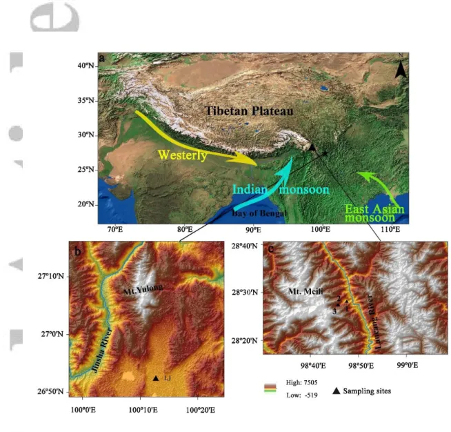
In this study, we present daily precipitation samples and their isotopic composition in the southeastern TP, in Mount Yulong (at Lijiang) and Mount Meili regions (Fig. 1). The region is located at the convergence of air masses between the westerlies and monsoon flows from the Bay of Bengal and the South China Sea (Fig. 1a). We investigate what controls the observed isotopic variability at the synoptic to seasonal time scale. Since our observations cover less than two years, the isotopic variability at the inter-annual time scale, which has already been analyzed in other studies (e.g. Ishizaki et al., 2012; Tan, 2014; Cai and Tian, 2016; Cai et al., 2017, 2019; Shao et al., 2017; Wang et al., 2020), is beyond the scope of this study. Compared to previous studies, our analysis goes further in testing the hypotheses on the physical mechanisms responsible for isotopic variations. First, we make use of existing satellite retrievals of water vapor and its isotopic composition to quantify the relative contributions from processes acting on the water vapor at the large-scale (here we define the “large-scale” as larger than the typical size of a general circulation model, e.g. 200 km), and local processes transforming the large-scale water vapor isotopic composition into the precipitation composition on the other hand. The satellite retrievals also allow us to gather a spatial view of isotopic variations and to assess the spatial coherence of the isotopic variability, which gives complementary information on the processes at play. Second, we filter the isotopic time series to isolate the isotopic variability at different time scales: synoptic, intra-seasonal and seasonal.
Isotope-enabled general circulation models are often used to help understand processes controlling the isotopic variability in precipitation (Risi et al., 2010a; He et al., 2015). To what extent are the different contributions to the δ2Hin precipitation (δ2H
p) variability over the TP
caught by the models? Does it depend on the time scale? Can these results shed some new light on the reasons for the difficulty of models to simulate the isotopic variability over the TP (e.g. Yao et al., 2013)? With this aim, we compare the observed isotopic variations to those simulated by several isotope-enabled general circulation models.
2 Material and methods
2.1 Material 2.1.1 Study area
Located in the southernmost of Hengduan Mountains Range, Mount Yulong (27º10'- 27º40' N, 100°9'-100°20' E) with the peak 5 596 m a.s.l. is a typical monsoonal temperate glacier region in China (Fig. 1a). Lijiang basin (26. 86° N, 100. 25° E, 2393 m a.s.l.) is just only 25 km south from Mount Yulong (Fig. 1b). The region is characterized by a typical monsoon climate. The south Asian/Indian monsoon results in abundant rains during the wet season (from May/June to October) with an average annual precipitation of 956.2 mm from 1951 to 2013. Monsoon winds are typically from the South, bringing water vapor from the Bay of Bengal (blue arrow in Fig. 1a) or from the South China Sea (green arrow in Fig. 1a). In contrast, less precipitation occurs in the dry season (from November to the next April) because of the dry and warm air brought by the south branch of the westerly (Pu et al., 2017, yellow arrow in Fig. 1a) with an average temperature of 12.8℃, and an average annual relative humidity of 63% (Shi et al., 2017).
To assess the spatial coherence of isotopic variability in precipitation at different time scales, we also collected daily precipitation samples at 3 sites in Mount Meili (28°33′-28°41′ N, 98°30′-98°40′ E, 6740 m a.s.l.), which is located around 210 km northwest of Mount Yulong and has similar climatic characteristics (Fig. 1c). The 3 sampling sites are Mingyong (28.47°, 98.79° E, 2306 m, MY), Taizimiao (28.46° N, 98.76° E, 2937 m, TZ) and Lianhuasi (28.46° N, 98.76° E, 3243 m, LH), respectively.
2.1.2 Sampling and isotopic analysis
Precipitation was sampled at the daily scale at 4 observation stations (Fig. 1). At Lijiang, precipitation was sampled from 19, March 2017 to 20, August 2018 (Fig. 2a). To assess the spatial coherence of the observed δ2H variability, precipitation was sampled at three other
stations located at different altitudes near Mount Meili, from 26, June 2017 to 31, July 2018 (MY), from 8, August 2017 to 1, August, 2018 (TZ), and from 16, July, 2017 to 1, August, 2018 (LH), respectively (Fig. 2b-d). We make no attempt to assign values into days without precipitation.
To be consistent with the time period of δ2H in water vapor retrieved from Infrared
Atmospheric Sounding Interferometer (see section 2.1.3), only the precipitation data in 2017 at Lijiang were analyzed in this study. This leaves us with 76 days where precipitation isotopic composition is analyzed. When assessing the spatial coherence of the observed δ2H variability,
and for this purpose only, the precipitation data for the whole sampling period of the 4 stations are used, so as to maximize the common periods between the four stations.
All precipitation samples were analyzed with respect to VSMOW at the Key Laboratory of Western China’s Environmental Systems (Ministry of Education), Lanzhou University, using a liquid water isotope analyzer (Picarro L2130-i). All 2H/1H ratios were expressed in
δ-notation, with the precision of 0.5‰ for δ2H.
2.1.3 Water vapor isotopic retrievals by satellite
The precipitation forms locally from water vapor, which records an integrated history of phase change processes along its trajectories. Therefore, it is instructive to separate the isotopic variability observed in precipitation into the isotopic variability in water vapor on the one hand, and the isotopic difference between water vapor and precipitation on the other hand. We thus need the isotopic composition of the water vapor. With this aim, we use isotopic retrievals from three different satellites.
We use δ2H retrievals from Infrared Atmospheric Sounding Interferometer (IASI, Lacour et al., 2012, 2015, 2018), which is currently the remote sensor with the best spatio-temporal sampling capabilities for δ2H retrieval. Each location is sampled twice daily, allowing
the δ2H variability in the vapor to be resolved at the synoptic scale. The horizontal footprint of IASI data is 12 km. Full tropospheric profiles are retrieved, but with very limited vertical resolution. We use δ2H retrievals at 5 km above ground level, close to the level of maximum
sensitivity of the retrievals. Since the IASI retrievals are very computationally expensive, retrievals were computed only for a restricted geographical domain (20-30º N, 94-106º E) for the year 2017.
To put the isotopic variations into a broader regional context, we use the δ2H retrievals
from Tropospheric Emission Spectrometer (TES, Worden et al., 2006, 2007) and Greenhouse gases Observing Satellite (GOSAT, Frankenberg et al., 2013). For TES, we use the optimized version that allows to retrieve vertical profiles with degrees of freedom spread throughout the troposphere (Worden et al., 2012). For consistency with IASI, we also use retrievals at 5 km above ground level. For GOSAT, we use the column-integrated δ2H, because no vertical
profiles can be retrieved from this technique. Since most of the total-column vapor is in the lower troposphere, column-integrated δ2H is strongly weighted towards the δ2H of the
boundary layer.
IASI, TES and GOSAT products are from clear-sky only. We select only profiles that reach several quality criteria. Specifically, for GOSAT measurements, we select measurements that met following quality criteria (Risi et al., 2013): no cloud; retrieved precipitable water (W) agrees within 30% with ECMWF reanalysis; errors on retrieved W and column-integrated HDO are lower than 15% (Frankenberg et al., 2013); retrieval χ2 is lower than 0.3; retrieved δ2H is within -900‰ and 1000‰ to exclude a few obviously anomalous values. For TES, we
select only TES measurements with a valid quality flag and a degree of freedom of the signal (DOFS) greater than 0.5. All these conditions reduce the spatio-temporal sampling. The TES measurements, retrieval methods and uncertainties are described in earlier studies (Worden et al., 2006, 2007; Risi et al., 2010a). Satellite products usually lack absolute calibration, and effectively show large offsets between each other (Risi et al., 2012). When interpreting TES, GOSAT and IASI retrievals, we only focus on temporal variability rather than on absolute values.
TES and GOSAT have a low spatio-temporal sampling, and were not available anymore in 2017. Therefore, we use these products to analyze the seasonal variations only, using multi-year-mean monthly values to describe the seasonal cycle. Years are 2004-2007 (corresponding to the period when the sampling frequency was maximum) for TES and 2009-2011 for GOSAT.
We acknowledge that the seasonal cycle of the isotopic composition may vary from year to year, in association with inter-annual variability modes such as El Nino Southern Oscillation (ENSO). However, for water isotopes, inter-annual variations are generally smaller than seasonal variations. We checked this both in precipitation and in the water vapor. For precipitation, we used the Tibetan Network for Isotopes in Precipitation (TNIP) data at Lhasa which covers 13 years from 1994 to 2006. The multi-annual-mean seasonality in δ18O (no observed δ2H data), quantified as the July-August minus March-April δ18O difference, is
-12.1‰, whereas the inter-annual standard deviation of the δ18O seasonality is 6.9 ‰. This
confirms that inter-annual variations are smaller than seasonal variations. For the water vapor, we assessed the robustness of the δ2H seasonality using 8 years of TES observations (2004-2011). Over most of the TP region and China, the multi-annual-mean seasonality in δ2H is larger than the inter-annual standard deviation of the seasonality (Fig. S1), including Lijiang with a factor 2. Therefore, this gives us confidence that the seasonal variations that we analyze with the TES and GOSAT datasets are robust and are informative even though the time periods
are different. Finally, note that the year 2017, when our precipitation was sampled at Lijiang and Mount Meili stations, was an ENSO-neutral year at the global scale (Ramirez and Briones, 2017).
We will show in the results section that at the seasonal scale, TES, GOSAT and IASI give results that are very smooth and spatially coherent. Results are noisier and less spatially coherent for IASI at the intra-seasonal and synoptic time scales. To assess to what extent this noise and weaker spatial coherence are physical and not artifacts due to errors, we performed an extensive error analysis detailed in Appendix 1, including errors associated with the instrument sensitivity, random errors, and sampling biases in time and in space.
2.1.4 Meteorological observations
To look at the relationships between observed δ2H in precipitation and local
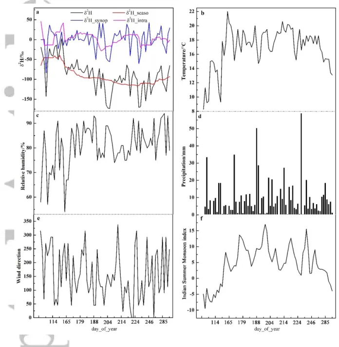
meteorological conditions, surface air temperature, precipitation amount and relative humidity data were used (Fig. 3b-d).
To assess the effect of the origin of air masses, we use wind direction at 15 m corresponding the daily maximum wind speed at Lijiang from the China Meteorological Data Service Center (CMDC). The wind direction, binned into 16 directions, was converted into direction in degrees between 0 and 360°, where the 0°-360° discontinuity corresponds to the North (Fig. 3e). The wind rose shows that the wind most often blows from the South-East or from the West (Fig. S2). The fact that the wind direction varies non-monotonically from 360° to 0° when going from North-Westerly to North-Easterly could be a problem when calculating correlations, because correlation analysis is designed to assess the relationships between monotonically varying variables. In our case, the fact that northerly wind is scarce prevents issues associated with this 360°-0° discontinuity.
To explore the influence of upstream convection on the δ2H in precipitation, daily
precipitation data from Tropical Rainfall Measuring Mission (TRMM, Huffman et al., 2007) is available for the sampling period with the spatial resolutions of 0.25°× 0.25°.
To access the influence of Indian monsoon, the Indian Summer Monsoon (ISM) index is also defined with the 850hPa zonal winds averaged over the southern Arabian Sea region (5°-15° N, 40°-80º E) minus that averaged over the northern region (20º-30º N, 70º-90º E) (Fig. 3f), reflecting the large-scale rainfall variability of the Indian summer monsoon (Wang et al., 2009; Gao et al., 2018). The 850hpa zonal wind data at 2.5°× 2.5° resolution are obtained from the NCAR/NCEP reanalysis data (Kalnay et al., 1996).
2.1.5 Model simulations
To assess the ability of isotope-enabled general circulation models (GCMs) to capture the seasonal isotopic variability at Lijiang, we use the outputs of nine simulations from seven isotope-enabled GCMs archived by Stable Water Isotope Intercomparison Group, Phase 2 (SWING2, Table S2) (Risi et al., 2012). The SWING2 simulations do not all have the same setup: some simulations are free-running and forced by observed sea surface conditions, whereas in others the horizontal winds are nudged towards reanalysis data to ensure a more realistic simulation of the large-scale circulation (Table S2). In addition, the period of the
simulations does not correspond to the data period. Therefore, the simulation set-up in available SWING2 simulations is not perfect for this data-model comparison. However, the seasonal variability that we investigate using these simulations is much larger than the year-to-year variability, as explained in section 2.1.3.
Only monthly outputs are archived in the context of the SWING2 project. Therefore, for outputs at the shorter time scale, we used simulations using the LMDZ5A version of LMDZ (Laboratoire de Météorologie Dynamique Zoom), which is the atmospheric component of the IPSL-CM5A coupled model (Dufresne et al., 2013) that took part in CMIP5 (Coupled Model Intercomparison Project). This version is very close to LMDZ4 (Hourdin et al., 2006). Water isotopes are implemented with the same way as in its predecessor LMDZ4 (Risi et al., 2010a). The simulation is forced by observed monthly sea-surface conditions and the winds are nudged towards the 6-hourly winds from the ECMWF operation analyses (Uppala et al., 2005). Such a simulation has already been described and extensively validated for isotopic variables in both precipitation and water vapor (Risi et al., 2010a; Risi et al., 2012). We use the outputs for the year 2017 to compare with in situ measurements at Lijiang.
2.2 Methods 2.2.1 δ2H filtering
Because the daily δ2H in precipitation combines the variability at different time scales, we decompose the isotopic changes into 3 different time scales: “seasonal”, “intra-seasonal” and “synoptic” scales (eg, Fig. 3a at Lijiang).
To do so, we filter the daily δ2H time series by applying a moving average with time
constants of 30 days and 10 days. The moving average acts as a low-pass filter. We note δ2H10
and δ2H30 as the 10 days and 30 days filtered δ2H time series respectively. The raw daily δ2H
time series is decomposed into seasonal (δ2H
seaso), intra-seasonal (δ2Hintra) and synoptic
(δ2Hsynop) components:
δ2H = δ2
Hseaso + δ2Hintra + δ2Hsynop
where δ2Hseaso is calculated as δ2Hseaso = δ2H30 andrepresents the “seasonal” part of the
δ2H variability, δ2H
intra is calculated as δ2Hintra = δ2H10 - δ2H30 and represents the
“intra-seasonal” part, and δ2H
synop is calculated as δ2Hsynop = δ2H - δ2H10 and represents the “synoptic”
part (Fig. 3a).
All other time series (eg. Fig. 3b-f, temperature, relative humidity, wind direction…) can be filtered in the same way.
2.2.2 Precipitation δ2H decomposition
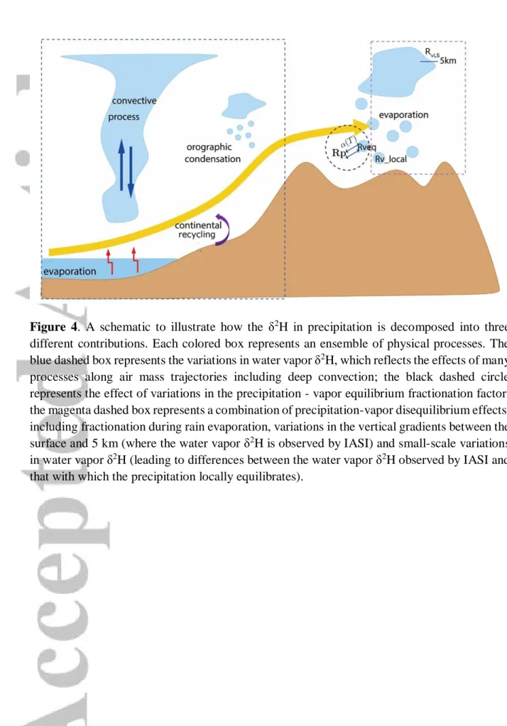
The goal is to decompose the daily-mean isotopic variability observed in the precipitation into the contribution from different processes (e.g, Botsyun et al., 2016) as illustrated in Fig. 4. We exploit the fact that we have water vapor δ2H observations from IASI for the same period as our precipitation δ2H, i.e. for the year 2017. First, we write the
precipitation isotopic ratio (Rp) as the isotopic ratio in equilibrium with the vapor (𝛼 ∙ 𝑅𝑣𝐿𝑆) plus a residual:
𝑅𝑝 = 𝛼 ∙ 𝑅𝑣𝐿𝑆 + (𝑅𝑝− 𝛼 ∙ 𝑅𝑣𝐿𝑆) (1)
α is the equilibrium fractionation coefficient that depends on temperature (Majoube, 1971) .
RvLS is estimated from IASI retrievals at 5 km altitude. Every day, we average allprofiles in
a 3.6°x2.5° grid box. In average, there are 26.5 profiles per day in the Lijiang grid box. Therefore, RvLS represents the isotopic composition of the vapor at the large scale, hence the
subscript “LS”. We define
𝑅𝑣𝑒𝑞 = 𝑅𝑝⁄𝛼 (2)
where Rveq is the isotopic composition of vapor under precipitation - vapor equilibrium.
We further decompose α into its temporal mean over the full sampling period (𝛼) plus its anomaly (𝛼′):
𝛼 = 𝛼 + 𝛼′ (3) Rearranging equations yields:
𝑅𝑝 = 𝛼′∙ 𝑅
𝑣𝑒𝑞+ 𝛼 ∙ 𝑅𝑣𝐿𝑆+ 𝛼 ∙ (𝑅𝑣𝑒𝑞− 𝑅𝑣𝐿𝑆) (4) In delta notation, this yields:
𝛿2𝐻𝑝 =𝛼′∙𝑅𝑣𝑒𝑞 𝑅𝑠𝑚𝑜𝑤 ∙ 1000 + ( 𝛼∙𝑅𝑣𝐿𝑆 𝑅𝑠𝑚𝑜𝑤 − 1) ∙ 1000 + 𝛼∙(𝑅𝑣𝑒𝑞−𝑅𝑣𝐿𝑆) 𝑅𝑠𝑚𝑜𝑤 ∙ 1000 (5)
The first term on the right-hand side represents the effect of variations in the precipitation-vapor equilibrium fractionation factor (Fig. 4, black dashed circle). The second term represents the effect of variations in water vapor δ2H at the large-scale. These variations
integrate all processes along air mass trajectories (Fig. 4, blue dashed square). The third term (Fig. 4, magenta dashed square) represents a combination of precipitation-vapor disequilibrium effects (due to variations in condensation altitude or post-condensation processes such as rain evaporation), variations in the vertical gradients between the surface (where the precipitation achieves its last equilibration, e.g. Graf et al., 2019) and 5 km (where the water vapor δ2H is
observed by IASI) and small-scale variations in water vapor δ2H (leading to difference between the water vapor δ2H observed by IASI and that with which the precipitation locally
equilibrates).
This decomposition can be applied on raw time series, or on filtered time series (section 2.2.1). In any case, all variables in Eq. (5) are filtered at the same time scale and following the same procedure.
2.2.3 Back trajectory analysis and cumulated precipitation along trajectories
Many previous studies have shown the relationship between δ2Hp and precipitation
upstream air mass trajectories (Vimeux et al., 2005; Risi et al., 2008b; Gao et al., 2013; He et al., 2015). To assess this effect, we compute daily back trajectories from Lijiang based on a 2D trajectory algorithm (Vimeux et al., 2005) and ECMWF ReAnalysis - Interim (ERA-I) (Dee et al., 2011) 6-hourly meridional and zonal wind fields. Each day, a trajectory is calculated with time steps every 6 hours backward in time, up to 7 days.
TRMM precipitation was cumulated along the n previous days along each trajectory, n varying from 1 to 7. This yields a time series of cumulated precipitation along trajectories.
3 Results
3.1 δ2H time series and relationship with local meteorological variables
Daily δ2Hp vary greatly from -173.5‰ to 2.4‰ during the sampling period, with a
weighted-average value of -99.5‰ (Fig. 2a). Precipitation isotope is enriched from November to May, corresponding to the non-monsoon season, and depleted from June to October, corresponding to the Indian monsoon season. This is consistent with the previous studies in the southeastern TP (Yu et al., 2016b; Pang et al., 2006; Pu et al., 2017).
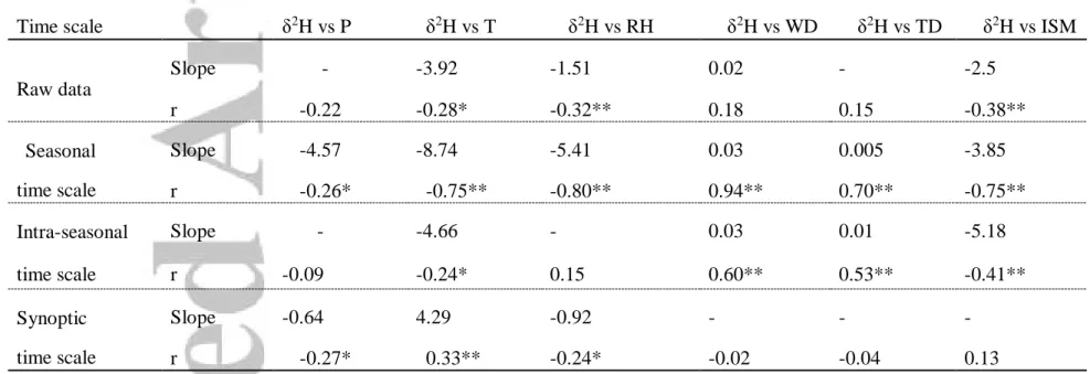
In order to further asses what controls the variability of precipitation δ2H at different time scales (seasonal, intra-seasonal and synoptic scale), we analyze the relationships between δ2H
p and local meteorological factors (eg, temperature, precipitation amount, relative humidity
and wind direction) (Table 1). In particular, the local temperature and precipitation amount are often explored as possible factors controlling the δ2Hp in the southern TP (Pang et al., 2006;
Yao et al., 2013; Yu et al., 2016a). The intensity of the monsoon is also often cited (Wang et al., 2009; Gao et al., 2018), quantified here by the ISM. Note that when calculating correlations between two variables, regardless of whether they are isotopic or metrological variables, we always ensure that these two variables cover the same time period and that the smoothing time scale is the same.
At all the time scales, the correlation between δ2Hp and local precipitation is weak (r
=-0.26, p< 0.05 at the seasonal scale, r=-0.27, p<0.05 at the synoptic scale), discarding the local amount effect as a major control of the δ2H
p variations. In contrast, the strong correlation
between δ2Hp and the ISM (r =-0.75, p<0.01 at the seasonal scale, r =-0.41, p<0.01 at the
intra-seasonal scale) suggests that the “amount effect” upstream air mass trajectories, associated with deep convection along trajectories, is an important factor. This is consistent with previous studies (Gao et al., 2013; He et al., 2015; Dong et al., 2016) that showed that local precipitation is not sufficient to explain the δ2H
p variability in the southern TP, and that upstream deep
convection is a more important factor (section 3.3). The correlation between δ2H
p and local temperature is very significant at the seasonal
of air masses, we would expect δ2H
p to increase with temperature (Dansgaard et al 1964). We
notice that this correlation is the same as between δ2H
p and the ISM, and that temperature and
the ISM are strongly correlated (r = 0.97, p<0.01, Table S3). Therefore, the link between δ2Hp
and temperature is probably simply a consequence of the link between δ2H
p and the ISM. The
correlation between δ2H
p and local temperature is also significant, though weaker, at the
synoptic scale (r=0.33, p<0.05). Such a positive correlation could be due to the distillation of air masses, or to the correlation of both δ2Hp and temperature with the local meteorological
situation.
The meteorological variable that correlates the most strongly with δ2H
p is local wind
direction (r=0.94, p<0.01 at the seasonal scale, r=0.60, p<0.01 at the intra-seasonal scale). Precipitation δ2H is more depleted during the monsoon season when air comes from the South,
and more enriched when the air comes from the West. This is consistent with the effect of moisture origin highlighted in several previous studies (Tian et al., 2007, 2008; Yu et al., 2008, 2014; Kong et al., 2019b). However, the local wind direction observed at Lijiang is more representative of the local circulation or meteorological situation than the large-scale circulation. The correlations between local wind direction and the direction of air mass trajectories (e.g. quantified as the direction of the vector connecting Lijiang from the trajectory location 3 days before its arrival, hereafter “trajectory direction”) are weak and significant only at the seasonal scale ( r = 0.69, p<0.01, Table S3). The correlations between δ2H
p and trajectory
direction are also significant, though weaker (r = 0.70, p<0.01 at the seasonal scale, r=0.53, p=0.01 at the intra-seasonal scale, Table 1). Therefore, both local wind direction associated with local circulation and meteorological situation, and to a lesser extent trajectory direction associated with the large-scale circulation and origin of air masses, emerge as important factors.
The second meteorological variable that correlates the most strongly with δ2H p is
relative humidity (r =-0.80, p<0.01 at the seasonal scale, r=-0.41, p<0.01 at the intra-seasonal scale). The lower correlation between relative humidity and the ISM indicates that this cannot be a simple consequence of the link between δ2H
p and the ISM. Relative humidity can impact
δ2H
p through two main mechanisms: first, low relative humidity is associated with stronger
subsidence that bring depleted water vapor downward (Frankenberg et al., 2009, Galewsky and Hurley, 2010). This would lead to a positive correlation opposite to what we observe. Second, low relative humidity drives stronger rain evaporation that enriches δ2H
p. This probably leads
to the negative correlation that we observe. Finally, it is also possible that both relative humidity and δ2H
p independently respond to the seasonal climate pattern and seasonal moisture
transport, in a way that is slightly different from the ISM. More generally, this correlation analysis is useful to hypothesize what processes drive the δ2H
p variability. However, a
correlation does not necessarily mean a causal relationship. To better understand whether rain evaporation is a major factor controlling the δ2Hp seasonality, we turn to our decomposition
method.
3.2 Decomposition of the variability in δ2H in precipitation
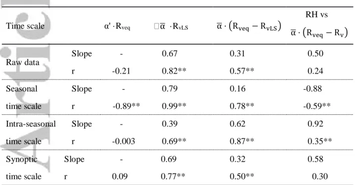
To better understand what process drive the precipitation δ2H variability, the raw and filtered time series are decomposed into 3 contributions as explained in section 2.2.2 and illustrated in Fig. 4. For example, Fig. 5 shows the raw precipitation δ2H time series and its 3
contributions. We can check that the sum of the 3 contributions (Fig. 5, black dashed line) yields the initial raw precipitation time series (Fig. 5, magenta). We can see that the first contribution α'·Rveq (Fig. 5, black), which represents the effect of temperature variations on precipitation-vapor equilibrium fractionation coefficient, is very small. It can be neglected. The second contribution 𝛼 · 𝑅𝑣𝐿𝑆 , and the third contribution 𝛼 · (𝑅𝑣𝑒𝑞− 𝑅𝑣𝐿𝑆) show large fluctuations, and their impact on the δ2H variability at different time scales can be quantified
by the correlation analysis that follows. Quantitatively, Table 2 summarizes the correlation coefficients and slopes of the three different contributions as a function of δ2H
p at different
time scales.
At the seasonal scale, δ2Hp is significantly correlated with the third contribution 𝛼 ·
(𝑅𝑣𝑒𝑞− 𝑅𝑣𝐿𝑆) (r=0.97, p<0.01). The slope indicates that it contributes to 69% of the δ2H p
variations (Table 2). This suggests that processes transforming the δ2HvLS variability into the
δ2H
p variability are the main drivers of seasonal variation in δ2Hp at Lijiang. This is consistent
with section 3.1 that suggested a key role for local processes, especially local circulation and rain evaporation. The role of local circulation is further supported by the correlation between the third contribution and local wind direction (r = 0.97, p < 0.01). The local circulation could drive small-scale vertical and horizontal heterogeneities in water vapor δ2H relatively to δ2HvLS.
The role of rain evaporation is also further supported by the correlation between the third contribution and relative humidity (r = -0.91, p < 0.01): as the air is drier, the precipitation evaporates more efficiently as it falls and gets more enriched relatively to δ2H
vLS.
Another prominent correlation at the seasonal scale is between δ2H
p and the second
contribution 𝛼 · 𝑅𝑣𝐿𝑆 (r=0.81, p<0.01). The slope indicates that it contributes to 27% of the δ2H
p variations (Table 2). This probably reflects convective processes along air mass
trajectories (section 3.3). This could also include an effect of the moisture origin: the second contribution also correlates significantly with local wind direction (r=0.62, p<0.01), which at the seasonal scale reflects both local and large-scale circulation (section 3.1, Table S3).
At the intra-seasonal scale, δ2Hp is significantly correlated with the third contribution
(r = 0.90, p<0.01). This indicates that processes transforming the δ2H
vLS variability into the
δ2H
p variability are the main drivers, contributing to 115 % of δ2Hp variations. This local
contribution may reflect both the effect of rain evaporation (r=-0.33, p<0.01 with relative humidity) and of local circulation (r=0.79, p<0.01). The fact that this contribution exceeds 100 % indicates that it is counter-balanced by another processes. It means that without the other counter-balancing process, the δ2H
p variability would be greater than observed. This
counter-balancing process is represented by the second contribution. Indeed, δ2Hp is negatively
correlated with the second contribution, indicating that processes along trajectories are not drivers. Rather, these processes blur or dampen the δ2Hp variability.
At the synoptic scale, processes transforming the δ2HvLS variability into the δ2Hp
variability dominate (r=0.46, p<0.01), contributing to 68% of the synoptic variability in δ2H p.
detected, we can discard a significant effect of rain evaporation. No significant correlation between the third contribution and local wind speed can be detected either, discarding an effect of local circulation. Small-scale vertical and horizontal heterogeneities in water vapor δ2H, associated with local meteorological conditions, could be the main drivers of this contribution.
Could errors in IASI affect our result that processes transforming δ2HvLS into δ2Hp
emerge as the most important contribution at all time scales? Actually, IASI errors tend to lower the contribution of this contribution (Appendix 1). Therefore, in reality we may expect an even larger contribution of these processes.
3.3 Relationship with upstream convection
To test the hypothesis that at the seasonal scale deep convection upstream air mass trajectories is also a key driver of δ2H
p variations, daily TRMM precipitation is cumulated
along the n previous days along each air mass trajectories. The temporal correlation between δ2H
p and δ2HvLS and cumulated precipitation amount is shown as a function of n (Fig. 6).
At the seasonal scale, δ2Hp is significantly anti-correlated with the cumulated
precipitation amount from 1 to 3 days preceding the rainy event. The strongest negative correlation is obtained for n = 2 days (r = -0.89, p < 0.01). δ2HvLS exhibits a similar pattern,
which is remarkable given that precipitation and water vapor δ2H are from completely independent sources of data. This result is consistent with previous studies highlighting the important role of deep convection along air mass trajectories in the TP region (Table S1), and in other monsoon regions of the world (Vimeux et al., 2005; Risi et al., 2008a, b; Vimeux et al., 2011; Tremoy et al., 2012).
Air mass trajectories are associated with the monsoon flow in the lower troposphere. The mechanisms by which deep convection depletes the lower tropospheric water vapor along the air mass trajectories have already been documented in previous observational and modeling studies. First, convective or meso-scale downdrafts bring depleted water vapor from the free troposphere downward (Risi et al., 2008b, 2010a; Kurita et al., 2013). Second, rain evaporation in moist conditions and diffusive exchanges between the rain and vapor deplete the water vapor (Lawrence et al., 2004; Worden et al., 2007; Field et al., 2010; Lacour et al., 2018).
At the intra-seasonal and synoptic scales, there is no significant anti-correlation with the cumulated precipitation. This is consistent with the result of the previous section suggesting that at these time scales, the observed variability is not driven by processes affecting the large-scale water vapor, but rather by local processes transforming the large-large-scale water vapor variability into the precipitation variability. However, at the intra-seasonal scale, we observe a significantly positive correlation between water vapor δ2H and cumulated precipitation for all lags. We do not know how to interpret this correlation. We can’t find any physical mechanisms that would lead to such a correlation.
3.4 Spatial scale of isotopic variability in precipitation and vapor
To test whether the local processes produced the short-term variation in precipitation and vapor δ2H, we use three different datasets. 1) TES and GOSAT datasets are used to show
the seasonal difference of δ2H in vapor at the scale of China and nearby countries (Fig. 7); 2) IASI daily output of δ2H in vapor is used to show the spatial coherence of water vapor δ2H
variations from the seasonal to synoptic scale; 3) Observed daily precipitation isotope in Mount Yulong and Mount Meili are used to access the spatial scale of isotopic variability.
The TES and GOSAT data show that the seasonal variations observed at Lijiang, with more depleted precipitation in the monsoon season (July-August) than before the monsoon onset (March-April), are also observed in a wide region from about 18°N to 30°N and 85°E to 120°E (Fig. 7). The deep convection associated with the Indian monsoon occurs over a wide region, thus impacting the water vapor δ2H over a wide region as well.
The IASI observations allow us to assess the spatial imprint of the δ2H variability at the
seasonal to synoptic scales (Fig. S3). At the seasonal scale, the water vapor δ2H at Lijiang correlates significantly with the water vapor δ2H everywhere around (r>0.8), consistent with the fact that the seasonality of water vapor δ2H has a very wide spatial imprint. At the
intra-seasonal scale, the correlations are significant over a smaller region of a few hundreds of kilometers (r>0.4). At the synoptic scale, the correlations become insignificant everywhere (r<0.4), consistent with purely local processes controlling the variability.
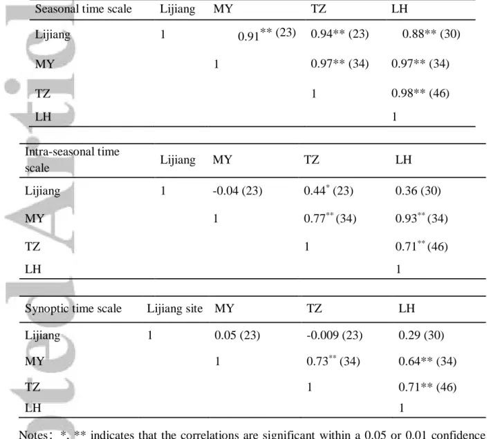
To further assess the spatial coherence of the δ2H variability, precipitation δ2H at Lijiang is compared with that observed at 3 other sites distributed at different altitudes (Fig. 1, section 2.1.1). The correlation for each pair of sites is calculated at different time scales (Table 3). At the seasonal scale, δ2H
p at Lijiang is strongly correlated with δ2Hp at the 3 sites at Mount
Meili (r>0.88, p<0.01, Table 3). This is consistent with the large-scale imprint of the seasonal variations.
At the intra-seasonal scale, a robust positive correlation (p<0.05) is observed only between δ2Hat Lijiang and TZ in Mount Meili (Table 3). This confirms that the spatial scale of intra-seasonal variations is smaller than for seasonal variations. At the synoptic scale, there is no relationship between Lijiang and the three sites at Mont Meili, supporting the small spatial scale of synoptic variations and thus the importance of local processes.
To summarize, the shorter the time scale of isotopic variations, the smaller the spatial imprint of these variations.
3.5 Comparison with isotope-enabled general circulation models
We have quantified the relative contributions of different processes to the isotopic variability at Lijiang, and have assessed their spatial imprint. To what extent are these different contributions captured by the models?
At the seasonal scale, most models participating in SWING2 capture the seasonal cycle (Fig. 8, Table 4, r > 0.49 between observed and simulated δ2H at Lijiang for each model) because to some extent all models are able to capture the Indian monsoon and the associated depleting effect of deep convection. Qualitatively, the seasonality simulated by SWING2 models shows a large spatial coherence (Fig. S4), consistent with the pattern exhibited by
satellite observations (Fig. 7). The capacity of GCMs to simulate the seasonality of δ2H further supports the importance of processes that have a large spatial imprint i.e. convection integrated several days along trajectories or air mass origin. However, we note that many models underestimate the seasonal variations observed at Lijiang (Fig 8; Table 4: the slopes of simulated vs observed monthly δ2H
p are all lower than 1) and more generally in the monsoon
domain of the Tibetan Plateau and more generally in the monsoon domain of the Tibetan Plateau (Fig. S4 compared with Fig. 7). This underestimation had already been noticed in previous studies focusing on δ2Hp in China (Che et al., 2016), and more generally in the
monsoon domain of the Tibetan Plateau (Gao et al., 2011). These studies highlight the need for high horizontal resolution to properly simulate the observed δ2Hp depletion during the monsoon
season.
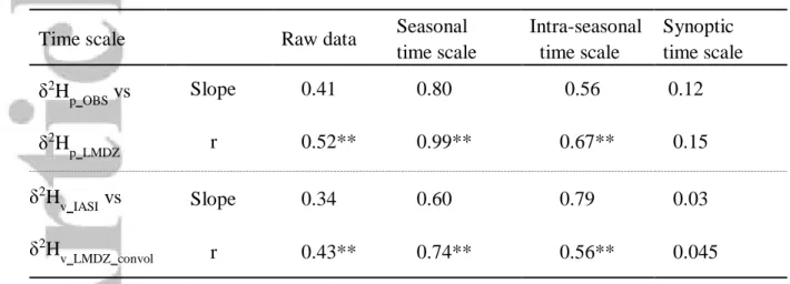
LMDZ results are consistent with those in SWING2 models. LMDZ can capture the seasonal cycle very well (r = 0.99, p < 0.01; Table 5, Fig. 9a), in spite of a slight underestimation of the amplitude (slope of 0.8). LMDZ also captures the δ2HvLS seasonal
variability observed by IASI, after taking into account the effect of instrument sensitivity (r=0.74, p<0.01, Fig. 9b, Table 5). The slightly lower correlation coefficient for the vapor can be explained by the different sources of IASI errors, namely random errors and sampling biases (Appendix 1).
We now investigate the driver of the δ2H
p seasonality in SWING2 models. In all models
but HadAM3_free, the main driver of δ2Hp is the 𝛼 ∙ 𝑅𝑣𝐿𝑆 contribution, at odds with
observations that show a dominance of local processes (section 3.2, Table 2). Most models underestimate the 𝛼 ∙ (𝑅𝑣𝑒𝑞− 𝑅𝑣𝐿𝑆) contribution (Table 4).
The same holds for LMDZ: processes along trajectories dominate in LMDZ (Table 6, 79%) and local processes transforming δ2HvLS into δ2Hp are secondary (Table 6, 16%). This is
in contrast with observations, which show that processes along trajectories dominate (section 3.2, Table 2). This mismatch cannot be due to errors from IASI (instrument sensitivity, random errors, sampling bias in time and in space). As shown in Table S7, errors in IASI tend to make the contribution of local processes weaker and even negative (Appendix 1, Table S7). Therefore, the mismatch is rather due to model shortcomings.
It is possible that a better horizontal resolution would improve the simulation of local processes transforming δ2HvLS into δ2Hp, enhance their contribution, and thus enhance the
seasonal amplitude of δ2H
p in better quantitative agreement with observations. Although
LMDZ underestimates the contribution of local processes, it seems to be able to capture the drivers of this contribution. The correlation between 𝛼 ∙ (𝑅𝑣𝑒𝑞− 𝑅𝑣) and relative humidity is -0.59, suggesting that in LMDZ, rain evaporation is a major driver of this contribution, consistent with observations (section 3.2).
To evaluate the capacity of GCMs to simulate the δ2Hp variability at the intra-seasonal
and synoptic scales, we use outputs from LMDZ. LMDZ can capture the intra-seasonal variations to some extent (r = 0.67, p<0.01) but underestimates them (slope of 0.56, Table 5). Similarly, it captures the δ2H
vLS variability observed by IASI, after taking into account the
effect of instrument sensitivity (r=0.56, p<0.1, Fig. 9b, Table 5). As for the seasonal scale, the slightly lower correlation coefficient for the vapor than for the precipitation can be explained by the different sources of IASI errors (Appendix 1). In contrast, LMDZ fails to capture the variability at the synoptic scale (r = 0.15).
LMDZ overestimate the 𝛼 ∙ 𝑅𝑣𝐿𝑆 contribution compared observations (Table 6 compared to Table 2): 39 % compared to -21 % at the intra-seasonal scale, and 69 % compared to a non-significant contribution at the synoptic scale. Considering IASI errors does not affect this conclusion (Table S7 compared to Table 6). Conversely, LMDZ underestimates the local processes that are encapsulated in 𝛼 ∙ (𝑅𝑣𝑒𝑞− 𝑅𝑣𝐿𝑆): 62 % compared to 115 % at the intra-seasonal scale and 32 % compared to 68 % at the synoptic scale (Table 6 compared to Table 2). Again, considering IASI errors would not change this conclusion (Table S7 compared to Table 8). The difficulty to represent this local contribution may explain the difficulty of LMDZ to capture the intra-seasonal and synoptic δ2Hp variability. It is possible that the coarse
resolution for LMDZ is not sufficient to represent the local processes transforming the δ2H vLS
variability into δ2Hp variability, for example local circulations or spatial heterogeneities in
δ2H
vLS at the small scale.
4 Discussion
4.1 Comparison with factors controlling precipitation δ2H in previous studies
Both sets of processes (processes along trajectories and local processes) had already been independently highlighted in previous studies. The importance of deep convection upstream trajectories in controlling the δ2H variations had already been reported in previous
studies, both in the southern -TP (e.g. Gao et al., 2013; He et al., 2015) and in other monsoon regions such as South America (Vimeux et al., 2005) and Western Africa (Risi et al., 2008a, 2010c). The importance of rain evaporation had also been pointed in the Southern TP (Ren et al., 2017) and in Western Africa (Risi et al., 2010b). These two processes are known to contribute to the amount effect (Risi et al., 2008b).
In this work, our study proposes a way to quantify the relative importance of these two sets of processes based on observations. At the intra-seasonal and synoptic scales, the dominance of local processes is in contrast with most previous studies that highlighted the effect of deep convection along trajectories at other sites in the Southern TP (e.g. Lhasa: Gao et al., 2013; He et al., 2015) and in other monsoon regions such as South America (Vimeux et al., 2011) or Western Africa (Risi et al., 2008, 2010a; Tremoy et al., 2012). This may be because of the complex terrain and diversity of trajectories in our region of interest. For example, in the Sahel, the terrain is essentially flat, and in South America, the air mass trajectories are less diverse (Vimeux et al., 2005). Our study also highlights the key role of
local circulations, in addition to the role of the large-scale circulation that had been highlighted in previous studies (Tian et al., 2007, 2008; Yu et al., 2008, 2014; Kong et al., 2019b).
4.2. Implications for the use of isotope-enabled models to study isotopic variability in the TP
All GCMs overestimate the effect of processes along trajectories affecting the water vapor composition at the large scale, whereas they underestimate the effect of local processes transforming this large-scale water vapor composition into local precipitation composition. Since local processes are increasingly important at shorter time scales, this may explain the difficulty of GCMs to simulate the δ2H
p variability at shorter time scales. Insufficient horizontal
resolution is a possible candidate for this shortcoming. Thus, to investigate what controls the isotopic variability at the synoptic time scales, an isotope-enabled model with much higher horizontal resolution would probably be needed (e.g. Moore et al., 2014, 2016; Dutsch et al., 2016, 2018).
4.3 Dependence on the time scale and implications for the interpretation of paleoclimate records
At the seasonal scale, the isotopic variation in precipitation and vapor is affected by the integrative effect of convective activity over several days preceding precipitation events, combined with a possible effect of air mass origin, but this is not the case at shorter time scales. This highlights the importance of separating the time scales when investigating the role of deep convection. If analyzing the correlations with the raw time series, we would have been misled to believe that the daily variability in δ2Hpis not associated with upstream deep convection,
whereas in reality the daily variability in δ2Hpat the seasonal scale is also affected by the
upstream deep convection.
Our study shows that the factors controlling δ2H variability strongly depend on the time
scale. Therefore, applying our results to interpret paleoclimate records is not obvious. A strong dependence on the time scale was also highlighted by Hu et al., (2019) between the inter-annual to the precessional time scales. Together with our results, this calls for caution when using relationships observed at short time scales to interpret paleoclimate records.
We show that local processes dominate at synoptic to intra-seasonal time scales. At the seasonal time scale, both local processes and processes along trajectories, including upstream deep convection, are important. We can thus hypothesize that processes along trajectories would dominate more and more at longer time scales. Our record is too short to show any results at the longer time scale, but previous studies confirm this hypothesis and have highlighted the dominance of processes along trajectories, especially the origin of air masses at the inter-annual time scale (Hu et al., 2019) and at the precessional and millennial time scales (Tabor et al., 2018) or upstream deep convection associated with ENSO at the inter-annual time scale (Ishizaki et al., 2012; Tan, 2014; Cai et al., 2016, 2017; Shao et al., 2017; Gao et al., 2018) and at the precessional and millennial time scales (Pausata et al., 2011; Lee et al., 2012; Battisti et al., 2014).
We show that the longer the time scale from synoptic to seasonal, the larger the spatial scale of variations recorded in precipitation δ2H (section 3.4). We may expect this to remain
true at scales even longer. The enhanced spatial coherence of precipitation δ2H at the inter-annual time scale, and even more at the precessional time scale, was already highlighted in Hu et al. (2019). At the glacial-interglacial time scale, the homogeneity of δ2H variations recorded in ice cores over tropical mountain regions around the globe is even more remarkable (Thompson et al., 2000b), which suggests that precipitation δ2H at such long paleo-climatic time scale may record a very large-scale variability, maybe at the tropical scale.
5 Conclusion
We have collected the daily precipitation samples at Lijiang in Mount Yulong region and at 3 sites in the Mount Meili region, and investigated what controls the isotopic variability at the seasonal, intra-seasonal and synoptic time scales based on a decomposition method using water vapor isotopic measurements by satellite.
At the seasonal scale, two kinds of processes control the variability in precipitation δ2H. First, processes along trajectories, particularly deep convection and the origin of air masses, affect the water vapor composition at the large scale. Second, local processes transform the isotopic variability in the large-scale water vapor into the local variability in the precipitation. These local processes may include small-scale spatial heterogeneities, variations in the vertical isotopic gradient, local circulation, condensation or post-condensation processes. Particularly, rain evaporation and local circulation emerge as important factors. At the seasonal scale, both kinds of processes have a large-scale spatial imprint.
At the intra-seasonal and synoptic scales, local processes dominate. The shorter the time scale of isotopic variations, the smaller the spatial imprint of these variations. We thus highlight the dependence of the isotopic drivers to the time scale of variability. Consequently, we emphasize the need to filter the time series to separate the different time scales. If we had analyzed the raw daily scale only, we would have been misled to over-estimate the importance of deep convection upstream trajectories at short time scales, and to underestimate its importance at the seasonal scale.
Isotope-enabled general circulation models can qualitatively capture the seasonal variations in δ2H, but they underestimate the contribution of local processes and overestimate the contribution of processes along trajectories. Local processes that impact the isotopic variability are underestimated at the intra-seasonal and synoptic scale by LMDZ with a coarse resolution, explaining its difficulty to reproduce the observed variations at these time scales.
Appendix 1: Sources of errors in δ2H retrieved by IASI
The goal is to assess the impact on the results of different sources of errors affecting the IASI observations. We quantify different sources of errors, and the impact of these sources of errors on our results. We cannot compare the results we would get with and without errors in IASI, since the real δ2H is not known. Therefore, we compare what we would get with and
without IASI errors in LMDZ. We note δ2Hv_LMDZ the δ2Hv simulated by LMDZ, and δ2Hv_IASI
the δ2H
1.1 Effect of instrument sensitivity
Due to limited instrument sensitivity, the retrieved profiles are smoothed versions of the true profiles. The averaging kernels describe the vertical sensitivity of the retrieval at each level to the true state at each level (Worden et al 2006; Risi et al., 2012). These depend on the atmospheric state. Therefore, part of the δ2H variability measured by satellites can be attributed to the variability in instrument sensitivity. To quantify this effect, we calculate the water vapor δ2H that IASI would retrieve if it was flying over the atmosphere of LMDZ. We co-locate
LMDZ outputs with IASI retrievals and we convolve these outputs by averaging kernels. We note the resulting time series δ2H
v_LMDZ_convol.
As expected, δ2Hv_LMDZ_convol is smoothed compared to δ2Hv_LMDZ, with the amplitude
of variations in δ2H
v_LMDZ_convol being 89 %, 95 % and 86 % with those in δ2Hv_LMDZ at the
seasonal, intra-seasonal and synoptic scales (Table S4).
At all the time scales, the correlation coefficients between δ2Hv_LMDZ_convol and δ2Hv _IASI
are better than between δ2H
v_LMDZ and δ2Hv_IASI (Table S4). This is consistent with the fact that
IASI observations are affected by instrument sensitivity compared to true profiles, and that we correctly account for this effect when calculating δ2H
v_LMDZ_convol.
1.2 Effect of random errors
IASI δ2H measurements are affected by random errors (Lacour et al., 2012). The typical standard deviation for these errors is 40‰ in the TP. Therefore, at longer time scales, more samples are considered in the average, and thus the impact of random errors on average values is lower. Specifically, when averaging n samples, we expect the error on the average to be divided by √n. The fact that IASI is noisier and less correlated with LMDZ at short time scale may be an artifact of those random errors.
To estimate the impact of these errors on the observed variability, we use a Monte-Carlo approach in which we add random errors to LMDZ outputs. For each retrieved profile i, we draw a random number ε(i) from a Gaussian distribution with a null mean and a standard deviation of 40‰. We add this number to the δ2H value that is simulated by LMDZ for this
day t, 𝛿2𝐻̂𝐿𝑀𝐷𝑍(𝑡):
δ2Herr(i) =δ2ĤLMDZ(t)+ ε(i) (A1) where the δ2H
err(i) is the 𝛿2𝐻 value that is distorted by the random error. Throughout
this appendix, the hat sign represents the daily average and the overbar sign represents the annual average.
We calculate a daily δ2H time series 𝛿2𝐻
𝑒𝑟𝑟(𝑡)
̂ by averaging all the δ2H
err (i) values
that belong to each given day. Finally, we estimate the correlation between the 𝛿2𝐻𝐿𝑀𝐷𝑍̂(𝑡) and 𝛿2𝐻̂𝑒𝑟𝑟(𝑡) time series. On average, 26.5 retrieved profiles in the Lijiang grid box are included in daily averages. This limits the effect of random errors. On average
over 10 Monte-Carlo simulations, the correlation coefficients between the 𝛿2𝐻𝐿𝑀𝐷𝑍̂(𝑡) and 𝛿2𝐻̂𝑒𝑟𝑟(𝑡) are 0.998, 0.974, 0.868 at the seasonal, intra and synoptic scales. Therefore, random errors may slightly distort δ2Hv_IASI time series at the synoptic scale, but not at longer
time scales.
1.3 Effect of diurnal cycle
IASI observations with a global coverage are generally retrieved twice a day (orbits crossing the Equator at 9:30 and 21:30 LT). To estimate the impact of the diurnal cycle of water vapor isotopic composition, the time series of water vapor δ2H are calculated based on morning and afternoon profiles separately. We decompose the daily-mean, grid-mean δ2H, 𝛿2̂ time series into : 𝐻(𝑡)
𝛿2̂ = 𝑃𝐻(𝑡) 𝑚(𝑡) ∙ 𝛿2̂𝐻𝑚(𝑡)+ (1 − 𝑃𝑚(𝑡)) ∙ 𝛿2̂ (A2) 𝐻𝑎(𝑡)
where 𝛿2̂ and 𝛿𝐻𝑚(𝑡) 2𝐻
𝑎(𝑡)
̂ are the daily-mean δ2H retrieved in the morning and in the afternoon and Pm(t) is the proportion of observations of water vapor in the morning on day
t. We further decompose Pm(t), 𝛿2𝐻
𝑚(𝑡)
̂ and 𝛿2𝐻
𝑎(𝑡)
̂ into the annual-mean 𝑃̅̅̅̅ , 𝛿𝑚 2𝐻
𝑚 ̅̅̅̅̅̅̅ and 𝛿2𝐻
𝑎
̅̅̅̅̅̅̅ plus their daily anomalies 𝑃𝑚(𝑡)′, 𝛿2𝐻
m(t)' and 𝛿2𝐻a(t)'. 𝑃𝑚(𝑡) = 𝑃̅̅̅̅ + 𝑃𝑚 𝑚(𝑡)′ (A3) 𝛿2̂𝐻𝑚(𝑡)= 𝛿̅̅̅̅̅̅̅ + 𝛿2𝐻𝑚 2𝐻𝑚(𝑡)′ (A4) 𝛿̂2𝐻𝑎(𝑡)= 𝛿̅̅̅̅̅̅̅ + 𝛿2𝐻𝑎 2𝐻𝑎(𝑡)′ (A5) We get the following decomposition:
𝛿2̂ = 𝑃𝐻(𝑡) 𝑚 ̅̅̅̅ ∙ 𝛿2𝐻 𝑚 ̅̅̅̅̅̅̅ + (1 − 𝑃̅̅̅̅) ∙ 𝛿𝑚 2𝐻 𝑎 ̅̅̅̅̅̅̅ + 𝑃𝑚(𝑡)′∙ (𝛿2𝐻 𝑚 ̅̅̅̅̅̅̅ − 𝛿2𝐻 𝑎 ̅̅̅̅̅̅̅) + 𝑃̅̅̅̅ ∙𝑚 𝛿2𝐻𝑚(𝑡)′+ (1 − 𝑃 𝑚 ̅̅̅̅) ∙ 𝛿2𝐻 𝑎(𝑡)′+ 𝑃𝑚(𝑡)′∙ (𝛿2𝐻𝑚(𝑡)′− 𝛿2𝐻𝑎(𝑡)′ ) (A6)
The first and second terms on the right-hand sides stand for the annual-mean δ2H in the morning and in the afternoon. The third term represents the effect of daily variations in the proportion of morning retrievals, named contrib_sampling. This represents the diurnal sampling bias. The fourth and fifth terms represent the effect of daily variations in the morning and in the afternoon δ2H, named contrib_signal. This is the physical variability in which we
are interested. The last term represents the effect of co-variability between the daily proportion anomalies and the δ2H anomalies in the morning and in the afternoon, named contrib_cross.
δ2H in the morning is correlated with δ2H in the afternoon, but it is systematically more
to the daily-mean δ2H variability is lower than 9% at all the time scales (Table S5, slopes of δ̂ vs contrib_sampling). The daily mean δ2H 2H is very well correlated with contrib_signal at
the seasonal and synoptic scales, but it is lower, though significant, at the intra-seasonal scale (Table S5). This means that the distortion of the daily-mean δ2H variability by the diurnal sampling bias is slight.
1.4 Effect of inhomogeneous spatial sampling
In the daily δ2H time series, every day represents an average of profiles that are located in a 3.6°x2.5° grid box. Inhomogeneous sampling in space can distort the daily-mean δ2H time
series if for some days, more profiles are located where the water vapor is more depleted or more enriched. At the scale of the grid box in such a mountainous region, we assume that the ground altitude z is the main controlling factor that leads to spatial variation of δ2H within the grid box (Bowen et al., 2010). How variable are the altitudes at which the IASI profiles are located? What is the impact of this variability on the daily δ2H time series? This is what we
aim at quantifying here.
We thus decompose the altitude range into nz small intervals, each representing altitudes z to z+dz (nz = 40, dz = 0.2 km, first interval starting at altitude z = 0 km). For each day t, the daily-mean, grid-mean 𝛿2𝐻, δ2̂ is given by: H(t)
𝛿̂ 2𝐻(𝑡)= ∑𝑛𝑧 𝑝(𝑡, 𝑧) ∙ 𝛿2𝐻(𝑡, 𝑧)
𝑧=1 (A7)
where p(t, z) is the probability density function for a given day t and altitude interval z and δ2H (t, z) is the daily mean δ2H for a given day t and altitude interval z.
We further decompose p(t, z) and δ2H (t, z) into their annual averages and their anomalies :
𝑝(𝑡, 𝑧) = 𝑝(𝑧)̅̅̅̅̅̅ + 𝑝(𝑡, 𝑧)′ (A8)
𝛿2𝐻(𝑡, 𝑧) = 𝛿̅̅̅̅̅̅̅̅̅ + 𝛿2𝐻(𝑧) 2𝐻(𝑡, 𝑧)′ (A9)
where 𝛿̅̅̅̅̅̅̅̅̅ and p(z) represent the annual-mean 𝛿2𝐻(𝑧) 2𝐻 and probability density functions when binned as function of z.
𝛿̅̅̅̅̅̅̅̅̅̅̅ =2𝐻(𝑧) ∑𝑛𝑡𝑡=1𝑝(𝑡,𝑧)∙𝛿2𝐻(𝑡,𝑧)
∑𝑛𝑡𝑡=1𝑝(𝑡,𝑧) (A10) 𝑝(𝑧)̅̅̅̅̅̅ = ∑𝑛𝑡 𝑝(𝑡, 𝑧)
𝑡=1 (A11)
and 𝑝(𝑡, 𝑧)′ and 𝛿2𝐻(𝑡, 𝑧)′ represent the daily anomalies of p(t,z) and 𝛿2𝐻 (t, z): 𝛿2𝐻(𝑡, 𝑧)′ = 𝛿2𝐻(𝑡, 𝑧) − 𝛿̅̅̅̅̅̅̅̅̅ (A12) 2𝐻(𝑧)
𝑝(𝑡, 𝑧)′ = 𝑝(𝑡,𝑧)