HAL Id: hal-00304857
https://hal.archives-ouvertes.fr/hal-00304857
Submitted on 13 Oct 2005
HAL is a multi-disciplinary open access
archive for the deposit and dissemination of
sci-entific research documents, whether they are
pub-lished or not. The documents may come from
teaching and research institutions in France or
abroad, or from public or private research centers.
L’archive ouverte pluridisciplinaire HAL, est
destinée au dépôt et à la diffusion de documents
scientifiques de niveau recherche, publiés ou non,
émanant des établissements d’enseignement et de
recherche français ou étrangers, des laboratoires
publics ou privés.
Spatial and temporal patterns of land surface fluxes
from remotely sensed surface temperatures within an
uncertainty modelling framework
M. F. Mccabe, J. D. Kalma, S. W. Franks
To cite this version:
M. F. Mccabe, J. D. Kalma, S. W. Franks. Spatial and temporal patterns of land surface fluxes
from remotely sensed surface temperatures within an uncertainty modelling framework. Hydrology
and Earth System Sciences Discussions, European Geosciences Union, 2005, 9 (5), pp.467-480.
�hal-00304857�
www.copernicus.org/EGU/hess/hess/9/467/ SRef-ID: 1607-7938/hess/2005-9-467 European Geosciences Union
Earth System
Sciences
Spatial and temporal patterns of land surface fluxes from remotely
sensed surface temperatures within an uncertainty modelling
framework
M. F. McCabe1, J. D. Kalma2, and S. W. Franks2
1Department of Civil and Environmental Engineering, Princeton University, Princeton, New Jersey, 08544, USA
2Discipline of Civil, Surveying and Environmental Engineering, School of Engineering, University of Newcastle, Callaghan
NSW 2308, Australia
Received: 14 March 2005 – Published in Hydrology and Earth System Sciences Discussions: 20 April 2005 Revised: 31 August 2005 – Accepted: 21 September 2005 – Published: 13 October 2005
Abstract. Characterising the development of
evapotranspi-ration through time is a difficult task, particularly when util-ising remote sensing data, because retrieved information is often spatially dense, but temporally sparse. Techniques to expand these essentially instantaneous measures are not only limited, they are restricted by the general paucity of infor-mation describing the spatial distribution and temporal evo-lution of evaporative patterns. In a novel approach, tem-poral changes in land surface temperatures, derived from NOAA-AVHRR imagery and a generalised split-window al-gorithm, are used as a calibration variable in a simple land surface scheme (TOPUP) and combined within the Gener-alised Likelihood Uncertainty Estimation (GLUE) method-ology to provide estimates of areal evapotranspiration at the pixel scale. Such an approach offers an innovative means of transcending the patch or landscape scale of SVAT type models, to spatially distributed estimates of model output. The resulting spatial and temporal patterns of land surface fluxes and surface resistance are used to more fully under-stand the hydro-ecological trends observed across a study catchment in eastern Australia. The modelling approach is assessed by comparing predicted cumulative evapotranspira-tion values with surface fluxes determined from Bowen ratio systems and using auxiliary information such as in-situ soil moisture measurements and depth to groundwater to corrob-orate observed responses.
Correspondence to: M. F. McCabe
1 Introduction
Early attempts at determining spatial distributions of evapo-transpiration at regional scales were often based on geostatis-tical and interpolation procedures (e.g. kriging and splines), using data from sparsely distributed meteorological stations to produce large scale maps of evapotranspiration and other hydrological variables. Alternatively, when regional water balance closure was attempted, estimates of evapotranspi-ration were generally determined as the difference between long-term rainfall and runoff. In more recent times, a vari-ety of modelling approaches have been developed to estimate evapotranspiration at both field and regional scales (Zhang et al., 1995; Li and Lyons, 1999; Braun et al., 2001), with these types of approaches generally relying on the broad ap-plication of effective parameter values to large homogeneous units of the land surface. Parameter uncertainty or sensitivity (Beven and Binley, 1992; Franks and Beven, 1997; Gupta et al., 1999) is rarely considered, thus the accuracy of predicted values cannot be assessed.
There is a general belief that remote sensing offers the most amenable means towards obtaining spatial evapotran-spiration patterns, although there exists little agreement on
how best to realise this. While numerous schemes and
methodologies have been proposed to provide estimates of land surface fluxes using surface temperatures obtained from remote sensors (Diak and Whipple, 1995; Anderson et al., 1997; Norman et al., 2000), estimation of evapotranspiration in this way has achieved varied levels of success. Whether this is due to the disparity between the aerodynamic and ra-diometric temperatures, to conceptual misrepresentations or to the inevitable scale issues that plague hydrological mod-elling, heat fluxes estimated in this way are often subject to significant uncertainty. Undoubtedly, successful measure-ment of surface fluxes with remote sensing techniques would
provide a valuable information source, and much progress is being made towards achieving this (e.g. Norman et al., 2003; Su et al., 2005). The ability to calibrate land surface mod-els and hence refine model predictions at larger spatial scales using such measurements would see an immediate improve-ment over existing techniques.
Humes et al. (2000) investigated a technique to provide maps of surface energy fluxes for two small watersheds lo-cated in different climatic conditions. A novel aspect of their approach was the use of spatial maps to identify the dominant factors controlling the energy fluxes for time periods shortly after precipitation events. The authors found that in the semi-arid environment studied, the patterns of sensible heat across the watershed were similar to that of the spatially variable cumulative precipitation. In contrast, sensible heat flux pat-terns in the sub-humid watershed tended to be more uniform and were influenced by a combination of precipitation and land cover type. The use of data in a qualitative way can of-ten be as informative as techniques designed to quantitatively examine spatial patterns, particularly given the uncertainties evident in model structure and input data and inconsisten-cies between observed and modeled variables. McCabe et al. (2005c) presented an intuitive example of the qualitative use of hydrological data sets by evaluating satellite soil mois-ture estimates using distributed precipitation patterns. The pattern rich information present in remote sensing data of-fers much potential for such application, but relatively little effort has been directed towards examining this. Qualitative evaluation of models is one aspect of a move towards ap-proaches that incorporate remote sensing as an alternative or proxy source of calibration information. The attraction of such a temporally consistent and spatially dense source of data is evident, given the paucity of ground based evaluation data available over much of the Earth.
Franks and Beven (1997) presented a methodology for the representation of spatial variability in land surface fluxes us-ing LANDSAT data and a simple SVAT model. Usus-ing mul-tiple realisations of the TOPUP model (Beven and Quinn, 1994), they classified the numerous model outputs into a number of functional types with different surface behaviour. Pixel scale flux estimates calculated from the satellite plat-form were then used to map surface fluxes across the land-scape using a fuzzy-disaggregation scheme – in effect map-ping the landscape space of the satellite estimates into the model space of the TOPUP functional types. Such an ap-proach represents a novel way in which a patch based model can be used to spatially disaggregate the modelled distribu-tion of surface fluxes across a landscape, whilst incorporat-ing both model and image uncertainty. The TOPUP model was particularly well suited to this style of spatial disagggation, as it accounts for a range of possible landscape re-sponses by producing multiple model realisations. Informa-tion from satellite platforms or other ground based sources can then be used to identify the likely landscape responses from the many possible model outputs using traditional
cali-bration techniques.
The information content that is present in a temporal record of surface temperature has been largely ignored in cal-ibration and modelling studies, with most techniques prefer-ring instantaneous remotely sensed temperatures in energy balance equations to determine surface flux predictions. Re-cent work (McCabe et al., 2005a), illustrated that the tempo-ral change in surface temperature can provide a useful tool for the calibration of a simple land surface model. The au-thors showed that by using observed infrared temperature differences to calibrate against modelled aerodynamic tem-perature, a significant reduction in the a priori uncertainty bounds of the latent heat resulted, facilitating improved pre-diction of surface fluxes. The work presented in this paper extends this concept using spatially distributed surface tem-perature differences derived from the NOAA-AVHRR plat-form as a means to identify land surface behaviour through-out a study catchment.
Many practically based models of evaporation rely on estimates of the potential evaporation, from which the ac-tual evaporation can be derived using a variety of correc-tion factors. Wallace (1995) commented that evapotranspi-ration studies should employ techniques that calculate the evaporation using the surface resistance directly – such as the physiological resistance to water vapour transport used in the Penman-Monteith equation. Surface resistance describes the physiological controls that plants have on water vapour transport on its route from inside the leaf, through the stom-atal openings and ultimately into the bulk atmosphere. The complexity in modelling such controls is obvious, as stom-atal response is a function of the moisture demand of the plant, the moisture conditions of the soil and atmosphere, as well as the time of day and season. Given the difficulty in measuring this variable and the important role it plays in evaporation studies, empirical relationships have been sought between the surface resistance and leaf cover, soil water sta-tus and a number of other environmental variables (Nemani and Running, 1989; Shuttleworth and Gurney, 1990; Jiang and Islam, 1999). Through the close relationship between the surface resistance and evapotranspiration, it is expected that the temporal and spatial patterns of this variable should corroborate the calibrated latent heat flux results, and also al-low insight into its dynamic nature during periods of varied hydrometeorology.
This paper addresses the use of remotely sensed sur-face temperature differences within an uncertainty modelling framework to predict spatial patterns of evapotranspiration. Further, through undertaking a calibration of the land sur-face model with observations of the sursur-face temperature, an assessment of the spatial distribution and temporal response of the surface resistance to variable hydro-climatic forcing is achieved. The results obtained from this calibration exercise are compared using flux data obtained from Bowen ratio
de-rived in situ measurements located in a 275 km2catchment
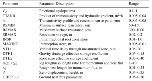
Table 1. TOPUP model parameterisation for the Drop Zone field investigation.
Parameter Parameter Description Range
FA Fractional upslope area 0.1–1
TTANB Product of transmissivity and hydraulic gradient, m2/h 0.005–0.04
m Transmissivity profile and recession curve parameter 0.005–0.05 RSMIN Minimum surface resistance, s/m 50–150 RSMAX Maximum surface resistance, s/m 300–1000 SRMAX Root zone storage, m 0.02–0.2 INSR Initial fractional root zone store 0.01–1.0 MAXINT Interception store, m 0.005–0.01 VTD Vertical time delay through unsaturated zone, h m−1 0.05–20 DTH1 Gravity drainage effective storage coefficient 0.05–0.15 DTH2 Root zone effective storage coefficient 0.05–0.40 ln(z0/zh) log roughness length ratio for momentum and heat flux 1–10 z0 Roughness length for momentum flux, m 0.01–0.25
d Zero displacement height, m 0.05–0.35 GHFP (ω) Ground heat flux parameter 0.05–0.20
2 Methodology
2.1 The TOPUP land surface model
The TOPUP model (Beven and Quinn, 1994; Franks et al., 1999) was developed to counter a trend towards more com-plex Soil Vegetation Atmosphere Transfer (SVAT) descrip-tions. The underlying rationale behind models of increased complexity is that improved process representation will yield parameters that are easier to measure or estimate and provide predictions that are more accurate. However, this is not nec-essarily the case for a number of reasons including (a) model parameters may not be equivalent to observed variables; (b) parameters that are physically represented may be difficult or impossible to measure (SVAT models aim to produce effec-tive values for the various parameters at patch, regional or larger scales and these cannot be easily estimated); and (c) issues of parameter inequality when moving between spatial and temporal scales remain unresolved.
The philosophy behind TOPUP details a move towards striking a balance between representing the key physical pro-cesses affecting land surface interactions while doing so in a parametrically parsimonious manner. The rationale for de-veloping a simplified model structure is that simplicity is necessary to validate the use of SVAT models in the field. Limited calibration data is available for such purposes, again highlighting the significant parametric and predictive un-certainty which exists in the general calibration, or more precisely, in the evaluation of SVAT models. This prob-lem is compounded for more complex model structures that are grossly over-parameterised with respect to the available calibration-evaluation data sets (Jakeman and Hornberger, 1993).
The dominant hydrological processes affecting evapotran-spiration have been incorporated into TOPUP in the simplest representation possible, whilst retaining a physically realistic conceptual foundation. Similar to many SVAT models, the water availability is controlled by a single bucket type storage function. TOPUP also includes a representation of the lateral redistribution of water flow across the model ‘patch’, an im-portant contribution of water supply in many landscapes, al-though not a significant consideration within the study area. TOPUP consists of three main moisture stores representing a vegetation interception, root zone storage and a variable, or dynamic, water table. These provide four main pathways for evaporation to proceed including; (1) evaporation from the interception store; (2) evapotranspiration from the root zone store; (3) evapotranspiration supplied by capillary rise from the water table; and (4) evapotranspiration from the water table when it is in the root zone (see Fig. 1a).
Water is routed through the system in a simple linear gression, modelling as closely as possible the physical pro-cess of water redistribution within the vertical profile. For example, given a sample rain event, the incident rainfall will initially be routed into the interception store until its capac-ity (MAXINT) is reached. At this point, moisture is then di-rected into the root zone storage until exceedence of the con-trolling parameter SRMAX is reached. Finally excess water from the root zone is routed to the water table, with a ver-tical time delay parameter (VTD), controlling the flow time. Given that the land surface at the research field site was con-sistently flat, the assumption of a minimal hydraulic gradient was employed. Thus, the lateral subsurface flow components within the model were not utilised for this study. Figure 1 presents a schematic of many of the processes described here and Table 1 an outline of the major parameters employed in TOPUP operation.
Evapotranspiration from the root zone store
(depth SRMAX) Evapotranspiration from
the water table when in the root zone Evapotranspiration supplied by capillary rise
from the water table Evaporation from the interception store (capacity MAXINT) (a) SRMAX Capillary Fringe Interception Storage (MAXINT) REFLEV (b) (c) RSMAX RSMIN Decreasing root zone storage
Fig. 1. Schematic of (a) the four pathways available to
evapotran-spiration within TOPUP; (b) a description of the sub-surface param-eterisations for root zone storage (SRMAX), maximum water table depth (REFLEV) and maximum interception storage (MAXINT);
(c) a representation of the linear decrease in surface resistance as
determined by the decrease in moisture availability in the root zone storage.
Within TOPUP, the surface resistance is a dynamic vari-able that is calculated at each time step according to the mois-ture content of the model’s three water stores. The surface resistance is assigned a value of 0 s/m when the interception store is at a maximum. As moisture within the interception store (canopy) is evaporated, rs is increased linearly up to a value of RSMIN. The parameter RSMIN expresses the sur-face resistance of an empty interception store (dry canopy) which is not limited by water supply. Once the interception store has been depleted, the water available for evapotran-spiration is then a function of the moisture content of the root zone, capillary rise through the unsaturated zone from the water table and from the water table directly if it has in-tersected the root zone boundaries. In a similar way as de-scribed for the interception store, rsis increased linearly to a value of RSMAX (the maximum surface resistance) at which point the available moisture has reached a minimum and the vegetation becomes water limited. Figure 1c illustrates the linear variation in surface resistance with changing moisture status.
In order to achieve closure of the surface energy balance, a series of equations have been used that allow determination of individual components of the energy balance as well as the aerodynamic surface temperature – of primary interest for the methodology proposed here. The equations characterise expressions for the surface energy balance and the latent and sensible heat flux, and are presented below:
Rn−G = H + LE (1) LE =ρcp γ (eo−e) rs (2) LE =ρcp γ (es[To] −eo) rs (3) H = ρcp(To −Ta) ra (4)
where Rnis the net radiation, LE, H and G are the latent,
sensible and ground heat fluxes (all in W/m2), Tois the aero-dynamic surface temperature, es[To], eoand e are the vapour pressures within the leaf stomata, at the leaf surface and of the bulk atmosphere respectively, rs is the surface resistance
and ra the aerodynamic resistance. ρ is the density of the
air, cpis the specific heat of air, and γ is the psychrometric constant. The soil, or ground heat flux component of the energy balance (G), has been represented in TOPUP as a function of the net radiation following studies by Clothier et al. (1986) who revealed that G follows a diurnal pattern closely matched to variations in the net radiation. The sub-model describing this process in TOPUP is relatively simple, demanding the specification of only one additional parame-ter, which restricts any unnecessary increase in the dimen-sions of the parameter space.
TOPUP requires standard meteorological forcing includ-ing net radiation, wind speed, air temperature, specific hu-midity and rainfall. Further details on the model and a more comprehensive review of the underlying physics and ratio-nale can be found in Franks and Beven (1997, 1999). A list of the required model parameters and the values used in this study is shown in Table 1.
2.2 Incorporating GLUE into a land surface model
While some land surface model parameters can be mea-sured directly, many others serve as conceptual represen-tations of a physical process and are not known precisely. One approach that has been proposed to address the problem of ill-defined process knowledge and model parameter un-certainty is the Generalised Likelihood Unun-certainty Estima-tion (GLUE) methodology (Beven and Binley, 1992), based on the concept of Generalised Sensitivity Analysis (GSA) (Spear and Hornberger, 1980). Whilst the aim of determin-istic modelling approaches is to identify an optimum param-eter set, GLUE recognises that many competing paramparam-eter combinations can adequately, if not equally well, reproduce the time series of specific model output – a concept known as equifinality. Although there are a number of subjective el-ements incorporated into the GLUE framework (such as the prior choice of parameter ranges, selection of an appropriate likelihood measure and in the specification of acceptability thresholds), GLUE does force these options to be made ex-plicit.
When parameters cannot be measured directly, which is the rule rather than the exception, broad ranges encom-passing expected parameter values can be identified, hence characterising the relative uncertainty in parameter measure-ments. The specification of feasible ranges for each model parameter recognizes the uncertainty inherent in land surface representations across a variety of scales. Multiple parame-ter sets can be constructed using Monte-Carlo sampling to
randomly extract parameter sets from the pre-defined ranges. Once parameter sets have been constructed (typically tens of thousands; in this investigation 20 000), the model is run with each set in turn. Assuming that some confidence in the model exists, it is reasonable to assume that within these multiple simulations are a number of model realisations that reflect the actual land surface observations. The issue then becomes one of how to distinguish those model outcomes that reflect what is actually occurring, from those that do not.
GLUE uses a simple likelihood measure to subjectively discriminate those model predictions and parameter sets that most closely reproduce observed variables. In essence, the process describes an evaluation of modelled data against available observations, employing a simple least squares er-ror analysis as the likelihood estimator. The choice of the least squares objective function was based on a number of studies that have employed it under the assumption of an er-ror model based on zero bias with normally distributed erer-rors (e.g. Kuczera, 1983). Using the least squares approach does not eliminate the risk of introducing bias in model identifi-cation. After each parameter set is run, a likelihood value is calculated for each model realisation, by comparing with cal-ibration/evaluation data. GLUE (like GSA) allows a thresh-old level on the least square estimator (or any other perfor-mance measure) to define behavioural/non-behavioural pa-rameter sets. In this application, the best 200 (or 1%) of model simulations are identified as the best performing re-alisations and discriminated for further analysis. More de-tailed descriptions of the GLUE methodology are provided in Franks and Beven (1997), Beven and Freer (2001) and specific to this investigation, in McCabe et al. (2005a).
2.3 Study area, ground based measurements and remote
sensing data
The study area in this investigation is located within the Tomago sand beds, a series of unconfined groundwater aquifers located on the mid-north coast of New South Wales, Australia, and encompassing an area of
approxi-mately 275 km2. Figure 2 details the aquifer extent, and
identifies adjacent water bodies. Vegetation communities within the Tomago region are varied and range from open forests and woodlands, to scrub, heath and mangrove com-munities. There are also a number of wetlands and extensive areas of grasslands, making this both an ecologically diverse and water sensitive environment. While many plant species in the area rely predominantly on the local water table for moisture supply, the ecology, environmental dynamics and continued viability of the system demands that the vege-tation be both resilient and tolerant to periods of drought. There have been few investigations into the effect that pro-longed lowering of the water table would have on plant com-munities, an issue made pertinent by planned commercial groundwater exploitation. Following the Koeppen classifica-tion system (Koeppen, 1931), the climate of the region was
Figure 1. Map of the Tomago sandbeds, a series of unconfined aquifers on the mid-north coast of New South Wales, Australia. The circled region identifies the location of the in-situ measurements.
0km 15km 30km
South Pacific Ocean
Fig. 2. Map of the Tomago sandbeds, a series of unconfined aquifers
on the mid-north coast of New South Wales, Australia. The cir-cled region identifies the location of the in-situ measurements and the central field site. The field site has approximate dimensions of 2 km by 1.5 km and is located near coordinates 151.5◦ longitude and 33.5◦latitude.
characterised as warm-humid-temperate, with rainfall spread evenly throughout the year and a mean annual precipitation varying between 1089 mm and 1257 mm. As is typical of much of Australia, pan evaporation exceeds rainfall for most of the year.
In order to gather information on the catchment for mod-elling purposes, an intensive data collection campaign was undertaken between December 2000 and March 2001. This collection period was preceded by an extended dry spell, with the first significant rainfall in a number of months occurring in late January. Following this, the remainder of the field campaign was characterised by sporadic rainfall events of varying intensity, interspersed with clear sky conditions, cre-ating a hydrologically informative wetting-up/drying-down dynamic. Additional data required for model forcing such as wind speed, net radiation, dry and wet-bulb temperature and rainfall, were obtained from measurements at a field site in the centre of the study region combined with regional mon-itoring at a nearby Australian Bureau of Meteorology cli-mate station. To determine model agreement after calibra-tion against observed variables, estimates of the latent heat flux were collected using a Bowen ratio system, located in a central location within the study region (see Fig. 2). These data provide an independent means of assessing the level of consistency between model results.
Remotely sensed surface temperatures were obtained from NOAA-12 and NOAA-14 AVHRR brightness temperature data at a resolution of 1 km, supplied by the Commonwealth Scientific and Industrial Research Organization (CSIRO)
Di-vision of Marine Research. Following techniques
docu-mented by Prata and Cechet (1999), surface temperatures in the Tomago region were calculated from this imagery using a simple split-window equation (McMillin and Crosby, 1984) and coefficients derived from multiple linear regressions of
the AVHRR data against a ground based infrared thermome-ter located within the study region. The infrared thermomethermome-ter samples radiation in a single window in the region 8–12 µm. Due to the limited field of view of these types of instruments (0.15 rad), the thermometer was mounted on a tower approx-imately 10 m above the ground surface, increasing the field of view to a diameter of 1.5 m at nadir configuration. As the thermometer was installed to allow comparison with diurnal trends extracted from a geostationary satellite, the instrument
housing was aligned to a viewing angle of 50◦. Land surface
temperatures calculated in this way were observed to have root mean square accuracies within 3 K. Further details of this analysis are offered below in Sect. 2.4.
2.4 Developing a calibration record using surface
tempera-tures
Land surface model predictions are more commonly evalu-ated against observations of surface heat fluxes. At regional and larger scales however, such data are rarely available at the pixel, let alone the regional scale, making model evalu-ation a difficult process. Calibrevalu-ation (or evaluevalu-ation) of pre-dictions with non-commensurate, or non-equivalent data, fa-cilitates the use of alternative sources of information such as land surface temperatures into the model assessment frame-work. Surface temperature measurements have the potential to yield significant insight into the surface dynamics when in-cluded within a modelling framework (e.g. Crow et al., 2004; McCabe et al., 2005a) as they are strongly coupled with a number of hydro-ecological processes. The use of tempera-ture differences to gain insight into the surface condition has its origins in thermal inertia studies, in which the time rate of change in the surface temperature is used to infer varia-tions in surface energy storage and to soil moisture status. The thermal inertia concept has been used in a determinis-tic manner to derive surface flux predictions (Wetzel et al., 1984; Diak and Whipple, 1995; Norman et al., 2000) and also to offer insight into soil moisture dynamics (McVicar and Jupp, 2002).
In order to implement a temperature difference approach to examine the spatial patterns of evapotranspiration across the study region, discrete temperature signatures were re-quired. McCabe et al. (2005a) used the difference between temperature observations at 1.5 and 5.5 h after sunrise, as suggested by Kustas and Humes (1996), who observed that this combination offers significant predictive insight into flux behaviour. The present study utilises NOAA-AVHRR data, limiting the capacity to calculate temperature differences to the 05:30 a.m. and 03:30 p.m. overpasses. While these are not the most ideal temperature pairs, it is expected that they should still offer some insight into flux behaviour. AVHRR temperature pairs at these times were discriminated for
use-able imagery. Following quality control criteria outlined
in Prata and Cechet (1999) and employed in McCabe et al. (2005b), which consider surface and atmospheric
influ-ences, low sensor angles and cloud affected imagery, ten brightness temperature pairs throughout January and Febru-ary were identified and extracted. Surface temperature esti-mates were then calculated using regressions to in situ mea-surements to parameterise the split-window equation. These techniques use combinations of a number of infrared chan-nels to determine surface temperatures from space, but re-quire physically based coefficients in order to transform the satellite brightness temperature to a surface skin temperature. Given the level of data availability in the study area, the the-oretically derived split-window approach represents the most suitable technique to determine the land surface temperature. Although there were a number of afternoon overpasses throughout the field campaign which were cloud free, some difficulties were encountered in obtaining early morning cloud free observations on the relevant days. The problem of morning cloud contamination was the primary limitation to using a greater number of image pairs. For larger scale ap-plications, not affected by land-surface/ocean boundaries as present here, the possibility of using geostationary platforms, such as in the work of Norman et al. (2003), should offer a more extensive and continuous source of calibration data.
2.5 Predictions of evapotranspiration and calculation of
surface resistance
The NOAA derived temperature pairs represent precisely
300 1 km2 land surface pixels, distributed across the
spa-tial domain of the study region (see Fig. 2). In effect,
this procedure generates three hundred unique calibration records, each containing ten clear sky surface temperature differences against which model output can be compared. Instead of analysing a single record of temperature differ-ences, as would be done for a traditional point-scale evalu-ation exercise, all responses derived from the AVHRR tem-perature records were used as evaluation data, each describ-ing a unique pixel within the region. In this way, numerous temporal records of observations (i.e. surface temperatures) are used to extract from the patch based land surface model a spatially distributed hydrological response (i.e. evapotran-spiration).
In order to capture the range of hydrological behaviour ex-pected at the regional scale, the TOPUP model was run nu-merous times using available meteorological forcing, with required model parameters sourced from the ranges speci-fied as part of the GLUE process. In this application, 20 000 unique parameter sets were constructed using Monte-Carlo random sampling from within the pre-defined parameter ranges (see Table 1) for the 51 days (or 2448 half-hourly time steps) of the field experiment. In order to compare model predictions with observation data, TOPUP-based tempera-ture differences were calculated for each of the 20 000 model runs corresponding to the times of the NOAA-AVHRR over-pass. While the modelled aerodynamic temperature and the observed radiometric temperature are not the same variable,
the difference between the two is expected to maintain some temporal consistency (Huband and Monteith, 1986; Basti-aanssen et al., 1998). Moran et al. (1997) indicate that these differences tend to be non-linear for non-vegetated surface. Over the region studied here, there are comparatively few such areas, increasing the confidence in the correlation of these variables.
After producing a temporally coincident series of model and observation outcomes, each of the 300 individual NOAA-AVHRR based evaluation records were compared to the 20 000 modelled simulations. A least squares likelihood function was used to discriminate those parameter sets that best reproduced the observed temperature differences from all possible outcomes. From these likelihood values, the best 200 (or 1%) of parameter sets were identified. This pro-cess was repeated for each of the 300 evaluation responses, thereby associating each pixel throughout the catchment with the best 200 parameter sets identified from the calibration process. From these sets, the mean cumulative ET and stan-dard deviations for each pixel over both the entire study pe-riod and for individual weeks throughout the campaign were determined. The following section presents the results of the spatial patterns of cumulative evapotranspiration derived from the temperature difference records, extending the anal-ysis to include an examination of another model output – the surface resistance patterns observed throughout the study re-gion.
3 Results
3.1 Spatial patterns of time changes in land surface
temper-ature
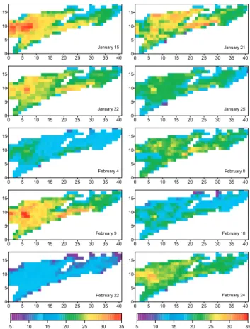
The spatial variation of clear sky temperature differences across the region for the ten clear days discriminated during the experimental period (Fig. 3) illustrate that there is a level of spatial structure evident throughout the region which is re-lated to the underlying surface vegetative conditions or land use. For instance, the regions towards the bottom-middle of the catchment (indicated by pixel coordinates x, y=5, 10) ex-hibit greater surface temperatures differences than surround-ing areas in the 15 January image. These pixels correspond to the relatively limited urban (built up) areas located within the catchment. The urban effects can be compared with the relatively lower temperature differences at the top end of the catchment (x, y=35, 13), where the surface is dominated by more established vegetation communities. The coastline, fol-lowing the lower edge of the study region, exhibits an in-creased temperature range than surrounding pixels due to the influence of sand dunes, which in some areas extend hun-dreds of metres from the shoreline.
The influence of variations in the moisture status of the catchment can also be observed. The images from the pre-dominantly hotter and drier January period contrast well with
0 4 5 3 0 3 5 2 0 2 5 1 0 1 5 0 0 5 0 1 5 1 5 1 y r a u n a J 0 4 5 3 0 3 5 2 0 2 5 1 0 1 5 0 0 5 0 1 5 1 1 2 y r a u n a J 0 4 5 3 0 3 5 2 0 2 5 1 0 1 5 0 0 5 0 1 5 1 2 2 y r a u n a J 0 4 5 3 0 3 5 2 0 2 5 1 0 1 5 0 0 5 0 1 5 1 5 2 y r a u n a J 0 4 5 3 0 3 5 2 0 2 5 1 0 1 5 0 0 5 0 1 5 1 4 y r a u r b e F 0 4 5 3 0 3 5 2 0 2 5 1 0 1 5 0 0 5 0 1 5 1 8 y r a u r b e F 0 4 5 3 0 3 5 2 0 2 5 1 0 1 5 0 0 5 0 1 5 1 9 y r a u r b e F 0 4 5 3 0 3 5 2 0 2 5 1 0 1 5 0 0 5 0 1 5 1 8 1 y r a u r b e F 0 4 5 3 0 3 5 2 0 2 5 1 0 1 5 0 0 5 0 1 5 1 2 2 y r a u r b e F 0 4 5 3 0 3 5 2 0 2 5 1 0 1 5 0 0 5 0 1 5 1 4 2 y r a u r b e F 5 10 15 20 25 30 35 5 10 15 20 25 30 35
Fig. 3. Spatial distribution of surface temperature changes (◦C) cal-culated as the difference between early morning (05:30 a.m.) and afternoon (03:30 p.m.) NOAA-AVHRR overpasses. x and y units are in kilometers and the images have a pixel scale of 1 km.
the generally cooler and wetter conditions prevalent during much of February. For instance, the images for 4, 18 and 22 February, correspond to periods after significant precipita-tion events across the catchment (17 mm, 13 mm and 27 mm, respectively). It is this feedback between the surface mois-ture status and the surface temperamois-ture response which forms much of the basis for the concept of thermal inertia.
The degree of spatial variation in the surface temperature differences on any one day is revealing, especially when spa-tial variability in model forcing data of air temperature (e.g. Prihodko and Goward, 1997) or net radiation (see Anthoni et al., 2000) is not routinely considered in land surface schemes. Clearly, there are correlations between the surface temper-ature and the underlying surface condition, which also im-pact on air temperature and net radiation. Even at the catch-ment scale studied here, it would be expected that through feedbacks within the surface temperature results alone, these forcing variables should also vary. Unfortunately, while as-sumptions of constant forcing data may increase uncertainty in predictions, there is generally little information available to spatially interpolate these variables from regionally sparse meteorological networks.
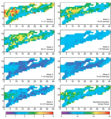
0 3 6 9 12 15 18 21 24 27 30 0 4 5 3 0 3 5 2 0 2 5 1 0 1 5 0 0 5 0 1 5 1 1 k e e W y r a u n a J 7 1 -1 1 0 4 5 3 0 3 5 2 0 2 5 1 0 1 5 0 0 5 0 1 5 1 2 k e e W y r a u n a J 4 2 -8 1 0 4 5 3 0 3 5 2 0 2 5 1 0 1 5 0 0 5 0 1 5 1 3 k e e W y r a u n a J 1 3 -5 2 0 4 5 3 0 3 5 2 0 2 5 1 0 1 5 0 0 5 0 1 5 1 4 k e e W y r a u r b e F 6 -1 0 4 5 3 0 3 5 2 0 2 5 1 0 1 5 0 0 5 0 1 5 1 5 k e e W y r a u r b e F 3 1 -7 0 4 5 3 0 3 5 2 0 2 5 1 0 1 5 0 0 5 0 1 5 1 6 k e e W y r a u r b e F 0 2 -4 1 0 4 5 3 0 3 5 2 0 2 5 1 0 1 5 0 0 5 0 1 5 1 7 k e e W y r a u r b e F 7 2 -1 2 0 4 5 3 0 3 5 2 0 2 5 1 0 1 5 0 0 5 0 1 5 1 T E e v it a l u m u C d o i r e P e r ti n E 0 0 1 120 140 160 180 200
Fig. 4. Spatial distribution of cumulative evapotranspiration (mm)
for individual weeks (left colour bar) and for the entire study period (right colour bar). x and y units are in kilometers and the images have a pixel scale of 1 km.
3.2 Spatial patterns of evapotranspiration
Spatially distributed maps of TOPUP calculated cumulative evapotranspiration are presented in Fig. 4, illustrating the patterns of the mean evapotranspiration over the two months of measurements and the individual weeks comprising this period. It is important to realise that actual pixel values repre-sent the mean of the two hundred cumulative ET values iden-tified as a result of the calibration process, based in this in-stance, on comparing modelled temperature differences with the satellite retrieved surface temperature differences. To understand the variability within the pixel responses, Fig. 5 presents the corresponding standard deviations. The cumu-lative evapotranspiration for the entire study period encom-passes the range 107–185 mm. During particular periods evaporative patterns are more closely linked to the underly-ing surface conditions, with the lowest evaporative rates oc-curring in the urban area. Such a result is entirely a function of the higher surface temperatures produced in this region, as no unique parameterisation of urban surface types was incor-porated into the TOPUP model.
The weekly evapotranspiration totals offer useful insight into the spatial and temporal variations across the watershed. As can be seen, the first three weeks indicate a degree of spa-tial variation that is not evident in the latter portion of the field campaign. In fact, the cumulative weekly evapotranspi-ration in Week 1 is perhaps higher than would be expected
0 4 5 3 0 3 5 2 0 2 5 1 0 1 5 0 0 5 0 1 5 1 1 k e e W y r a u n a J 7 1 -1 1 0 4 5 3 0 3 5 2 0 2 5 1 0 1 5 0 0 5 0 1 5 1 2 k e e W y r a u n a J 4 2 -8 1 0 4 5 3 0 3 5 2 0 2 5 1 0 1 5 0 0 5 0 1 5 1 4 k e e W y r a u r b e F 6 -1 0 4 5 3 0 3 5 2 0 2 5 1 0 1 5 0 0 5 0 1 5 1 5 k e e W y r a u r b e F 3 1 -7 0 4 5 3 0 3 5 2 0 2 5 1 0 1 5 0 0 5 0 1 5 1 6 k e e W y r a u r b e F 0 2 -4 1 0 4 5 3 0 3 5 2 0 2 5 1 0 1 5 0 0 5 0 1 5 1 7 k e e W y r a u r b e F 7 2 -1 2 0 4 5 3 0 3 5 2 0 2 5 1 0 1 5 0 0 5 0 1 5 1 n o it a i v e D d r a d n a t S d o i r e P e r it n E 0 1 2 3 4 5 5 10 15 20 0 4 5 3 0 3 5 2 0 2 5 1 0 1 5 0 0 5 0 1 5 1 3 k e e W y r a u n a J 1 3 -5 2
Fig. 5. Spatial distribution of the standard deviation of the mean
cumulative evaporation (mm) for individual weeks (left colour bar) and for the entire study period (right colour bar). The range of the standard deviation for Week 2 varies between 0 and 10. x and y units are in kilometers and the images have a pixel scale of 1 km.
given it is in the middle of a dry spell. The most likely ex-planation for this is the effect of a model parameter (INSR) that defines the fractional moisture of the initial root zone storage (SRMAX). INSR varies between zero for depleted root zone soil moisture and 1.0 for root zone soil moisture at capacity. Analysis of parameter sensitivity to various cali-bration records indicated that when calibrating model predic-tions to temperature differences, INSR shows some bias to-wards the upper range of the a priori parameter distribution. Thus, model runs would be initialised with an INSR value approaching unity, resulting in the higher evapotranspiration values evidenced in the results for Week 1. Knowledge of the antecedent conditions, such as soil moisture distribution from a satellite, could potentially be used to condition model outcomes. Alternatively, such information could be used in a multi-objective framework to co-condition model responses (see McCabe et al., 2005a).
Overall, results during the first three weeks reflect the hydrometeorological conditions characteristic for this hot and dry period, with weekly evaporative totals ranging be-tween 20–26 mm/week (generally less than 3 mm/day). Fig-ure 4 indicates that there is a reduction in the average weekly evaporative totals between Week 1 and Week 3 of approximately 6–10 mm/week (or 0.85–1.45 mm/day), iden-tifying the expected dry-down occurring during this pe-riod, confirmed through comparison with in situ measured
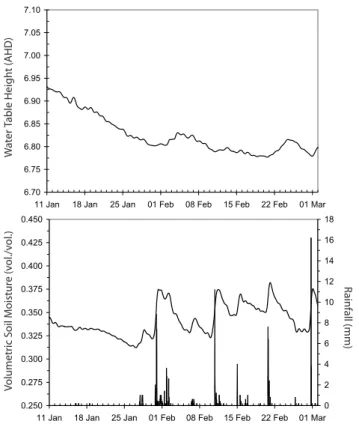
groundwater records (Fig. 6a). The average daily cumula-tive evapotranspiration estimated from Fig. 4 in the area en-compassing the location of the central field site (marked by the circle in Fig. 2) varies between 2.8 mm/day in Week 1 to 4 mm/day in Week 6. Measurements from the Bowen ra-tio system installed here offer some intermittent comparisons with these weekly values. Data collected from the system of-fered 21 days with which to compare model responses, with an average of 3 measurements per week. No in situ flux data was available for the first week and a half due to equipment related problems.
Independently measured flux data for Weeks 2 and 3 re-flect the low levels of evapotranspiration occurring during this period, with measurements indicating a high of 1.48 mm/day (25 January) and an average of 1.14 mm/day over this 2 week period. These values compare relatively well with results in Fig. 4, which indicate weekly evapotranspi-ration estimates in the range 10–15 mm (1.4–2.2 mm/day) at the field site. These results should be considered in light of accuracies typical of the Bowen ratio technique, which are often in the range of 20% (Kanemasu et al., 1992) depend-ing on field conditions. Field based measurements durdepend-ing February reflect the increased rates of evapotranspiration oc-curring in this period. Of the nine in situ measurements dur-ing Weeks 4 to 6, only 2 have values less than 3 mm/day, with the majority indicating totals greater than 4 mm. These correspond well to the TOPUP results, with estimates in the range 24–29 mm/week (3.4–4.2 mm/day). The drying down of the moisture stores is reflected in the data for Week 7, with an average value of 2.6 mm/day from the Bowen ratio measurements. This suggest a drop of nearly 10 mm/week compared to preceding weeks – a value which is supported by comparison with the overall spatial distributions evident in Fig. 4.
Overall, comparisons with available flux measurements indicate that the model is correctly capturing the observed hydrological dynamics evident throughout the study period. While Bowen ratio measurements were not available for Week 1, a trend consistent with both the observed hydrom-eteorology and surface temperature maps (Fig. 3) was evi-dent in the variation of the evaporative fraction (measured la-tent heat divided by the observed available energy) over the course of the investigation. For most of January, the aver-age evaporative fraction did not exceed 0.2, highlighting the dominance of sensible heat flux across the catchment, and the corresponding rise in observed surface temperatures. Af-ter the rainfall events of late January, the evaporative fraction reached a maximum value of 0.78. The varying dynamics oc-curring during February were reflected in the changing evap-orative fraction, which oscillated between 0.35 and 0.75 for the rest of the month, but generally exceeded 0.6.
Weeks 4–6 present a relatively uniform areal distribu-tion of evapotranspiradistribu-tion as a result of the sporadic rainfall events of varying intensity and the subsequent increase in soil moisture status throughout the catchment. These trends are
W
a
ter T
a
ble Height (AHD)
V
o
lumetric Soil Moistur
e (v ol./v ol.) R a infall (mm) 0 7 . 6 5 7 . 6 0 8 . 6 5 8 . 6 0 9 . 6 5 9 . 6 0 0 . 7 5 0 . 7 0 1 . 7 r a M 1 0 b e F 2 2 b e F 5 1 b e F 8 0 b e F 1 0 n a J 5 2 n a J 8 1 n a J 1 1 0 5 2 . 0 5 7 2 . 0 0 0 3 . 0 5 2 3 . 0 0 5 3 . 0 5 7 3 . 0 0 0 4 . 0 5 2 4 . 0 0 5 4 . 0 r a M 1 0 b e F 2 2 b e F 5 1 b e F 8 0 b e F 1 0 n a J 5 2 n a J 8 1 n a J 1 1 0 2 4 6 8 0 1 2 1 4 1 6 1 8 1
Fig. 6. Water table depth measured from ground level (top) and
daily rainfall and soil moisture trends (bottom) at the central field site. The water access tube for water table depth measurements has a surface datum at 8.40 m, from which measurements are taken relative to sea level (0.0 AHD).
reflected in Fig. 5b which illustrates both the rainfall events and soil moisture estimates determined from a probe located at the central field site. The results are consistent with ob-served increases in evaporative totals compared to earlier pe-riods of the investigation, with areal averages approaching 26–28 mm/week (approx. 4 mm/day). The spatial patterns il-lustrated in Week 5 and Week 7 reveal some insight into the drying dynamics of the catchment. As expected, as mois-ture availability is increased, so too is the evapotranspiration rate. However, this increased rate rapidly returned to pre-rainfall levels, at least within the time scales examined here, indicating that incident rainfall is swiftly evaporated from the surface, or infiltrates to the watertable.
The intermittent wetting and drying dynamics of the catch-ment, particularly throughout February, are prevalent in Fig. 4. The degree of variation is demonstrated through ref-erence to the standard deviations about the means shown in Fig. 5. Interestingly, the wetting and drying phases do not seem to significantly affect the variability in evaporative pre-dictions, at least in instances where the catchment moisture stores have been replenished. The standard deviations are linked with the prevailing meteorological conditions of the time, with dry periods exhibiting greater variability than oc-curs in wetter conditions. This is highlighted by an increased
11-Jan 13-Jan 15-Jan 17-Jan 19-Jan 21-Jan 23-Jan 25-Jan 27-Jan 0 100 200 300 400 500 600 700
27-Jan 29-Jan 31-Jan 02-Feb 04-Feb 06-Feb 08-Feb 10-Feb 12-Feb 0 100 200 300 400 500 600 700
13-Feb 15-Feb 17-Feb 19-Feb 21-Feb 23-Feb 25-Feb 27-Feb 01-Mar 0 100 200 300 400 500 600 700
Fig. 7. Mean values of the 5% and 95% quantiles of
evapotranspira-tion (W/m2)across the study region based on TOPUP simulations with 200 parameter sets at each pixel for each of the 2448 half-hourly time steps.
amount of standard deviation (relative to other periods) for Week 2. The range of the variation for this period is between 0 and 10 mm/week, as opposed to other periods which main-tain deviations less than 5 mm/week. February in general dis-plays minimal variation about the mean values, characteristic of the wetter catchment conditions, with standard deviations between 0.5–2 mm/week. In contrast, the drier January pe-riods produce standard deviations approaching 4 mm/week. These results are consistent with the ability of land surface models and remote sensing based approaches to predict evap-orative response. In general, the surface responses at limit-ing cases (i.e. soil controlled/atmospherically controlled) are easier to simulate than transitional periods, due primarily to uncertainties in partitioning the available energy.
Characterising prediction uncertainty is an often
over-looked component of model prediction. In remote
sens-ing based approaches for flux estimation, 50 W/m2 is often
cited as the useful accuracy limit for flux prediction (Kustas
and Norman, 2000). An uncertainty of 50 W/m2maintained
over a 12 h daylight period (as opposed to an instantaneous remote sensing based prediction) is equivalent to approxi-mately 0.9 mm of evapotranspiration. Understanding the un-certainty inherent in model applications is facilitated by
con-sidering the range of possible parameter realisations, as un-dertaken here using the GLUE methodology. With appro-priate calibration, it seems comparable accuracy can still be achieved using uncertainty based modelling approaches as in using remote sensing techniques.
3.3 Temporal changes in regional evapotranspiration
The uncertainty of regional scale estimates can be assessed through examination of the range of evaporative predictions throughout the catchment at an instant in time. Intuitively, it should be expected that when the moisture status of a catch-ment is high, the range of predicted evapotranspiration would be reduced, given that the surface evaporation approaches the potential rate. In contrast, a drier period should exhibit a greater degree of spatial variation and hence more areal un-certainty, as the influence of soil properties and vegetation dynamics exert greater control.
In the following analysis, uncertainty bounds are produced to describe the catchment response at each time step dur-ing the field campaign. At each of the 2448 half-hourly time steps, the range of evaporative predictions throughout the catchment is examined by considering the 200 model re-sponses identified by the likelihood analysis, for all of the 300 pixels defining the study region. The 5% and 95% quan-tiles are determined at each of these, and mean responses for the entire region calculated by averaging the 300 pixels at these two intervals. As a result, the subsequent ranges of values for each time step represent the 5% and 95% spa-tial quantiles of the areal mean evapotranspiration. Figure 7 illustrates the results of this process for the 2448 half-hour time steps of the TOPUP model run.
The greatest degree of spatial variation occurs in the period from 11–27 January. The clear sky days from 20–27 January indicate an areal difference in evaporation across the region of up to 300 W/m2at particular instances in time. This trend is consistent with the weekly spatial patterns evident in Week 2 and Week 3 (Fig. 4). As observed in Fig. 6, there was no rainfall before 27 January. After that date, intermittent pre-cipitation occurred, replenishing the depleted moisture stores throughout the catchment and reducing the spatial variability evident in the pre-rainfall evapotranspiration maps of Fig. 4. During the wetter month of February, the range of evapotran-spiration predictions throughout the catchment is reduced, with the difference between the 5% and 95% quantiles rarely
exceeding 200 W/m2 at the diurnal peak, but less than this
at other times. Indeed, most days have a range approaching
100 W/m2which, considering the variability in land surface
types and covers throughout the catchment, is not particu-larly large. Comparisons with the weekly evaporative trends (Fig. 4) and the standard deviations (Fig. 5), confirm the dy-namics of the temporal patterns displayed in Fig. 7. The spa-tial variability evident during drier periods is a function of the different drying dynamics throughout the catchment, which
in turn is related to soil properties and vegetation character-istics.
3.4 Regional patterns in surface resistance to
evapotranspi-ration
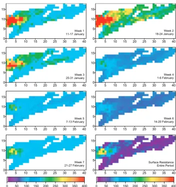
Following the same approach as for the evapotranspiration analysis described in Sect. 3.2, spatial maps of the surface resistance, a TOPUP model output, were produced for both the entire period and for weekly intervals throughout the field campaign. In order to graphically present the spatial varia-tion, mean values were calculated over each time period ex-amined. Because there were 200 associated responses for each pixel, an average pixel surface resistance was first cal-culated from within these responses, with results presented in Fig. 8.
While the response for the entire period is not particu-larly informative, the temporal development throughout the campaign exhibits some interesting trends. As reflected in the spatial evapotranspiration patterns, Week 1 shows a rel-atively even distribution of surface resistances, with values approaching 150 s/m and greater – likely a product of the cal-ibrated models preference for an increased initial moisture storage (see discussion in Sect. 3.2). It should be expected that the relationship between soil moisture status and evap-otranspiration would be strongly reflected in the surface re-sistance patterns. The dry conditions prevalent during much of January rapidly deplete the available soil moisture stor-age, allowing spatial patterns to become more evident during Weeks 2 and 3. In some parts of the catchment, values for the surface resistance approach 300 s/m during this drying period. The influence of the small amounts of precipitation that occurred at the end of January cause the spatial patterns displayed in Week 3 to reflect those in Week 1. During these first three weeks, the standard deviation of the modelled sur-face resistance – calculated from within the 200 samples for each pixel location – is generally within the range 25–50 s/m. Such a high value, relative to the mean surface resistance es-timate presented in Fig. 8, highlights the uncertainty of de-termining the surface resistance during these water limited conditions.
In contrast, the responses for most of February demon-strate a more uniform distribution of resistance values, with an average of approximately 100 s/m, and varying between 50 s/m and 200 s/m over the 4 week period. The effect of the intermittent drying and wetting phases of the surface is reflected in the variation throughout the weekly spatial pat-terns. The impact on the standard deviation also reflects the influence of precipitation on the surface resistance pattern. Weeks 4–7 display a marked reduction in the standard devi-ation across the catchment, with values approaching 10 s/m. Considering the variability in the first three weeks of the field campaign, this represents a significant reduction in the spatial and temporal uncertainty. The feedback between the surface
0 4 5 3 0 3 5 2 0 2 5 1 0 1 5 0 0 5 0 1 5 1 7 k e e W y r a u r b e F 7 2 -1 2 0 4 5 3 0 3 5 2 0 2 5 1 0 1 5 0 0 5 0 1 5 1 1 k e e W y r a u n a J 7 1 -1 1 0 4 5 3 0 3 5 2 0 2 5 1 0 1 5 0 0 5 0 1 5 1 2 k e e W y r a u n a J 4 2 -8 1 0 4 5 3 0 3 5 2 0 2 5 1 0 1 5 0 0 5 0 1 5 1 3 k e e W y r a u n a J 1 3 -5 2 0 4 5 3 0 3 5 2 0 2 5 1 0 1 5 0 0 5 0 1 5 1 4 k e e W y r a u r b e F 6 -1 0 4 5 3 0 3 5 2 0 2 5 1 0 1 5 0 0 5 0 1 5 1 5 k e e W y r a u r b e F 3 1 -7 0 4 5 3 0 3 5 2 0 2 5 1 0 1 5 0 0 5 0 1 5 1 6 k e e W y r a u r b e F 0 2 -4 1 0 4 5 3 0 3 5 2 0 2 5 1 0 1 5 0 0 5 0 1 5 1 e c n a t s i s e R e c a f r u S d o i r e P e r it n E 0 50 100 150 200 250 300 350 400 0 50 100 150 200 250 300 350 400
Fig. 8. Spatial distribution of the average surface resistance (s/m)
for both weekly averages and for the entire study period (bottom right). x and y units are in kilometers and the images have a pixel scale of 1 km.
resistance and evapotranspiration is well represented in the corresponding evapotranspiration maps of Fig. 4.
The temporal variation of surface resistances can be ex-amined in greater detail through discrimination of individ-ual pixel responses. Examination of these temporal patterns also offers an opportunity to qualitatively assess the perfor-mance of the land surface model. It is expected that the vegetative states of the surface should influence the tempo-ral development of the surface resistance, especially where drying of the moisture stores occurs. As such, the hydro-meteorological conditions experienced throughout the field campaign should be reflected in the temporal response of the surface resistance. To examine this further, Fig. 9 dis-plays the temporal trends of the 5% and 95% quantiles of surface resistance computed for two different vegetated sur-faces within the study region. The procedure employed here is the same as that for Fig. 7.
These two pixels were selected from a detailed land sur-face map of the dominant vegetation units throughout the re-gion (Woolley et al., 1995) and correspond to a swamp wood-land and heath and to a mixture of heath, swamp forest and open forest. As can be seen from Fig. 9, the more densely vegetated forested surface (bottom) displays a slower rise towards the peak surface resistance over the drying period from 11–28 January compared to that of the swamp wood-land/heath surface (top). Not only is the gradient reduced for this response, but so too is the maximum surface resistance
Time Step
15-Jan 22-Jan 29-Jan 05-Feb 12-Feb 19-Feb 26-Feb
Surface Resistance (s/m) 0 100 200 300 400 500 600
15-Jan 22-Jan 29-Jan 05-Feb 12-Feb 19-Feb 26-Feb
Surface Resistance (s/m) 0 100 200 300 400 500 600 Time Step Swamp Woodland/Heath Heath/Swamp Forest/Open Forest
Fig. 9. Time series of the 5% and 95% quantiles of the surface
resistance (s/m) for the duration of the field campaign for distinct vegeation units characteriistic of the catchment.
value, which peaks at approximately 400 s/m compared to 500 s/m. These same trends are reflected throughout the re-mainder of the study period, as the moisture status of the area is increased through precipitation during February and reduced during clear sky periods with strong surface drying between storm events.
Intuitively, these results are expected given the nature of the vegetation cover for each surface. The forested surface is likely to have deeper rooting depths than the swamp-heath land. As a consequence, the forest cover should be more tol-erant to a reduction in the moisture status, as occurs through-out January and for periods in February. However, there is insufficient information to reach any definitive conclusions on these patterns. Depth to the water table for instance, may bias results if one surface has a shallower water table than the other. Also, without further information on the vegetation characteristics of each of the surfaces, it is difficult to obtain more detailed insight. From a qualitative perspective, the re-duced bounds on the surface resistance during February are also reflected in the spatial patterns of Figs. 4 and 5. During
February, the spatial variability of the evapotranspiration is lower when compared to the drier January responses, which correspond to periods of greatest variability and uncertainty, in the surface resistance. This result was observed by Dol-man (1992) who comments that: “areal evaporation from dry regions is more sensitive to the spatial variability (in surface resistance) than evaporation from wet regions”.
4 Discussion and conclusion
Bastiaanssen et al. (1998) highlighted one of the major prob-lems associated with regional scale estimation techniques: how can regional evaporation predicted by simulation mod-els be validated with limited field data? They proposed that model verification can proceed through the use of in situ surface flux measurement, airborne flux measurement, soil moisture profiles in the field or through conventional hy-drological modelling. However, the majority of these tech-niques are generally the result of intensive field campaigns rather than through routine measurement. In most instances, the paucity of distributed measurements means that required information is not generally available to validate model re-sponses and hence most techniques remain unverified (e.g. Ottle et al., 1989; Smith and Choudhury, 1990), particularly at large spatial scales where data is simply not available. Clearly, an alternative approach is required to allow the as-sessment of large scale flux behaviour in a more operational, or routine, capacity.
A methodology that can be validated at the field scale and applied to the regional scale would prove very useful for model assessment and evaluation purposes. An ability to as-sess surface flux predictions using remotely sensed temper-atures offers much potential in land surface and in general climate modelling, where the scales at which processes are represented often preclude the actual measurement of sur-face fluxes for their validation. The development of evapo-transpiration patterns through time is of particular interest, given that there is generally a lack of information describ-ing both spatial and temporal evaporative patterns. While there are advances in providing increasingly accurate predic-tions of evapotranspiration directly from remote sensing vari-ables (Norman et al., 2003; Su et al., 2005), one of the major shortcomings of such approaches is that they remain essen-tially instantaneous retrievals. An approach which makes use of intermittent snapshots of the surface condition to expand knowledge of the surface flux throughout time would prove particularly useful.
The results from this study provide some evidence for the utility of spatially distributed satellite data in constraining predictions within an uncertainty modelling framework. Dis-tinct patterns of evapotranspiration were clearly observable throughout the study period, and insight into the close rela-tionship of the surface response to precipitation events was identified. The drying and wetting patterns throughout the
catchment, as observed in the spatial plots, also offered some insight into the surface resistance patterns throughout the re-gion. The dynamic response of the surface resistance to the catchment moisture status was evident through examination of the temporal plots and provided some corroboration for the model results throughout the duration of the field cam-paign.
The TOPUP land surface model represents a simple patch based approach, broadly parameterised to account for the range of responses expected from a heterogeneous surface. Through calibration against an observed record of surface temperatures, some insight into both the evapotranspiration patterns across the catchment, and also the temporal devel-opment of the surface resistance to evapotranspiration was
obtained. The fact that TOPUP was able to characterise
trends consistent with observed vegetation distributions, without having been explicitly spatially parameterised for these characteristics, is a significant result as it offers the possibility of parameterising models based on operationally
available remote sensing information. Such an approach
facilitates an increased opportunity to calibrate land surface models using a variety of remotely sensed hydrological variables, such as instantaneous evapotranspiration (e.g. Su et al., 2005), near surface soil moisture (e.g. McCabe et al., 2005c) or details on the land surface condition. Further investigations are in progress examining the utility of incorporating such remotely sensed information into a simplified representation of catchment processes to further our understanding of ungauged basins.
Edited by: A. Montanari
References
Anderson, M. C., Norman, J. M., Diak, G. R., Kustas, W. P., and Mecikalski, J. R.: A two-source time-integrated model for es-timating surface fluxes using thermal infrared remote sensing, Remote Sens. Environ., 60, 195–216, 1997.
Anthoni, P. M., Law, B. E., Unsworth, M. H., and Vong, R. J.: Varia-tion of net radiaVaria-tion over heterogeneous surfaces: measurements and simulation in a juniper-sagebrush ecosystem, Agric. For. Me-teorol., 102, 275–286, 2000.
Bastiaanssen, W. G. M., Menenti, M., Feddes, R. A., and Holtslag, A.: A remote sensing surface energy balance algorithm for land (SEBAL), I. Formulation, J. Hydrol., 212/213, 198–212, 1998. Beven, K. J. and Binley, A. M.: The future of distributed models:
model calibration and uncertainty prediction, Hydrol. Processes, 6, 279–298, 1992.
Beven, K. J. and Freer, J.: Equifinality, data assimilation, and uncer-tainty assessment in mechanistic modelling of complex environ-mental systems using the GLUE methodology, J. Hydrol., 249, 11–29, 2001.
Beven, K. J. and Quinn, P. F.: Similarity and scale effects in the water balance of heterogeneous areas, Paper presented at AG-MET conference on The Balance of Water – Present and Future, Dublin, Ireland, 1994.
Braun, P., Maurer, B., Muller, G., Gross, P., Heinemann, G., and Simmer, C.: An integrated approach for the determination of regional evapotranspiration using mesoscale modelling, remote sensing and boundary layer measurements, Meteorol. Atmos. Phys., 76, 83–105, 2001.
Clothier, B. E., Clawson, K. L., Pinter, P. J., Moran, M. S., Reginato, R. J., and Jackson, R. D.: Estimation of soil heat flux from net radiation during the growth of alfalfa, Agric. For. Meteorol., 37, 319–329, 1986.
Crow, W., Wood, E. F., and Pan, M.: Multi-objective cali-bration of land surface model evapotranspiration predictions using streamflow observations and spaceborne surface radio-metric temperature retrievals, J. Geophys. Res., 108, 4725, doi:1029/2002JD003292, 2004.
Diak, G. R. and Whipple, M. S.: Estimating surface sensible heat fluxes using surface temperatures measured from a geostation-ary satellite during FIFE 1989 – Note, J. Geophys. Res., 100, 25 453–25 461, 1995.
Dolman, A. J.: A note on the areally-averaged evaporation and the value of the effective surface conductance, J. Hydrol., 138, 583– 589, 1992.
Franks, S. W. and Beven, K. J.: Bayesian estimation of uncertainty in land surface-atmosphere flux predictions, J. Geophys. Res., 23 991–999, 1997.
Franks, S. W. and Beven, K. J.: Conditioning a multiple patch SVAT model using uncertain time-space estimates of latent heat flux as inferred from remotely sensed data, Water Resour. Res., 35, 2751–2761, 1999.
Franks, S. W., Beven, K. J., and Gash, J. H. C.: Multi-objective conditioning of a simple SVAT model, Hydrol. Earth Syst. Sci., 3, 477–489, 1999,
SRef-ID: 1607-7938/hess/1999-3-477.
Gupta, H. V., Bastidas, L. A., Sorooshian, S., Shuttleworth, W. J., and Yang, Z. L.: Parameter estimation of a land surface scheme using multicriteria methods, J. Geophys. Res., 104, 19 491– 19 503, 1999.
Huband, N. D. S. and Monteith, J. L.: Radiative surface temper-ature and energy balance of a wheat canopy, 1. Comparison of radiative and aerodynamic canopy temperature, Boundary Layer Meteorol., 86, 1–17, 1986.
Humes, K. S., Hardy, R., and Kustas, W. P.: Spatial patterns in sur-face energy balance components derived from remotely sensed data, Prof. Geographer, 52, 272–288, 2000.
Jakeman, A. and Hornberger, G.: How much complexity is war-ranted in a rainfall-runoff model, Water Resour. Res., 29, 2637– 2649, 1993.
Jiang, L. and Islam, S.: A methodology for estimation of surface evapotranspiration over large areas using remote sensing obser-vations, Geophys. Res. Lett., 26, 2773–2776, 1999.
Kanemasu, E. T., Verma, S. B., Smith, E. A., et al.: Surface flux measurement in FIFE: An overview, J. Geophys. Res., 97, 15 547–15 555, 1992.
Koeppen, W.: Klimakarte der Erde, Grundriss der Klimakunde, 2nd edition, Berlin and Leipzig, 1931.
Kuczera, G.: Improved parameter inference in catchment models, 1. Evaluating parameter uncertainty, Water Resour. Res., 19, 1151– 1162, 1983.
Kustas, W. P. and Humes, K. S.: Sensible heat flux from remotely-sensed data at different resolutions, in: Scaling up in Hydrology
using Remote Sensing, edited by: Stewart, J. B., Engman, E. T., Feddes, R. A., and Kerr, Y., John Wiley & Sons, 127–145, 1996. Kustas, W. P. and Norman, J. M.: Evaluating the effects of subpixel heterogeneity on pixel average fluxes, Remote Sens. Environ., 74, 327–342, 2000.
Li, F. Q. and Lyons, T. J.: Estimation of regional evapotranspira-tion through remote sensing, J. Appl. Meteorol., 38, 1644–1654, 1999.
McCabe, M. F., Franks, S. W., and Kalma, J. D.: Calibration of a land surface model using multiple data sets, J. Hydrol., 302, 209–222, 2005a.
McCabe, M. F., Prata, A. J., and Kalma, J. D.: A comparison of brightness temperatures derived from geostationary and polar or-biting satellites. Research Technical Report, Melbourne, VIC, CSIRO Division of Atmospheric Research, 63, 31 pp., 2005b. McCabe, M. F., Wood, E. F., and Gao, H.: Initial soil moisture
re-trievals from AMSR-E: Large scale comparisons with SMEX02 field observations and rainfall patterns over Iowa, Geophys. Res. Lett., 32, doi:10.1029/2004GL021222, 2005c.
McMillin, L. M. and Crosby, D. S.: Theory and validation of the multiple window sea surface temperature technique, J. Geophys. Res., 89, 3655–3661, 1984.
McVicar, T. R. and Jupp, D. L. B.: Using covariates to spatially interpolate moisture availability in the Murray-Darling Basin: A novel use of remotely sensed data, Remote Sens. Environ., 79, 199–212, 2002.
Moran, M. S., Humes, K. S., and Pinter, P. J.: The scaling charac-teristics of remotely-sensed variables for sparsely-vegetated het-erogeneous surfaces, J. Hydrol., 179, 337–362, 1997.
Nemani, R. R. and Running, S. W.: Estimation of regional surface resistance to evapotranspiration from NDVI and thermal infrared AVHRR data, J. Appl. Meteorol., 28, 276–284, 1989.
Norman, J. M., Anderson, M. C., Kustas, W. P., et al.: Remote sens-ing of surface energy fluxes at 10(1)-m pixel resolutions, Water Resour. Res., 39, 1221, doi:10.1029/2002WR001775, 2003. Norman, J. M., Kustas, W. P., Prueger, J. H., and Diak, G. R.:
Surface flux estimation using radiometric temperature: A dual temperature-difference method to minimize measurement errors, Water Resour. Res., 36, 2263–2274, 2000.
Ottle, C., Vidal-Majar, D. D., and Girard, R.: Remote sensing ap-plications to hydrological modelling, J. Hydrol., 105, 369–384, 1989.
Prata, A. J. and Cechet, R. P.: An assessment of the accuracy of land surface temperature determination from the GMS-5 VISSR, Remote Sens. Environ., 67, 1–14, 1999.
Prihodko, L. and Goward, S. N.: Estimation of air temperature from remotely sensed surface observations, Remote Sens. Environ., 60, 335–346, 1997.
Shuttleworth, W. J. and Gurney, R. J.: The theoretical relation-ship between foliage temperature and canopy resistance in sparse crops, Q. J. R. Meteorol. Soc., 116, 497–519, 1990.
Smith, R. C. G. and Choudhury, B. J.: Relationship of multi-spectral data to land surface evaporation from the Australian continent, Int. J. Remote Sens., 11, 2069–2088, 1990.
Spear, R. C. and Hornberger, G. M.: Eutrophication in Peel Inlet II. Identification of critical uncertainties via Generalised Sensitivity Analysis, Water Resour. Res., 14, 43–49, 1980.
Su, H., McCabe, M. F., Wood, E. F., Su, Z., and Prueger, J. H.: Mod-eling evapotranspiration during SMACEX02: comparing two ap-proaches for local and regional scale prediction, J. Hydrometeo-rology, in press, 2005.
Wallace, J. S.: Calculating evapotranspiration: resistance to factors, Agric. For. Meteorol., 73, 353–366, 1995.
Wetzel, P. J., Atlas, D., and Woodward, R.: Determining soil mois-ture from geosynchronous satellite infrared data: A feasibility study, J. Clim. Appl. Met., 23, 375–391, 1984.
Woolley, D., Mount, T., and Gill, J.: Tomago-Stockton-Tomarree Groundwater: Technical Review. Sydney, NSW Department of Water Resources, 160pp., 1995.
Zhang, L., Lemeur, R., and Goutorbe, J. P.: A one layer resistance model for estimating regional evapotranspiration using remote sensing data, Agric. For. Meteorol., 77, 241–261, 1995.