HAL Id: hal-02889665
https://hal.archives-ouvertes.fr/hal-02889665
Submitted on 15 Apr 2021
HAL is a multi-disciplinary open access
archive for the deposit and dissemination of
sci-entific research documents, whether they are
pub-lished or not. The documents may come from
teaching and research institutions in France or
abroad, or from public or private research centers.
L’archive ouverte pluridisciplinaire HAL, est
destinée au dépôt et à la diffusion de documents
scientifiques de niveau recherche, publiés ou non,
émanant des établissements d’enseignement et de
recherche français ou étrangers, des laboratoires
publics ou privés.
A Review of H2, CH4, and Hydrocarbon Formation in
Experimental Serpentinization Using Network Analysis
Samuel Barbier, Fang Huang, Muriel Andreani, Renbiao Tao, Jihua Hao,
Ahmed Eleish, Anirudh Prabhu, Osama Minhas, Kathleen Fontaine, Peter
Fox, et al.
To cite this version:
Samuel Barbier, Fang Huang, Muriel Andreani, Renbiao Tao, Jihua Hao, et al.. A Review of H2, CH4,
and Hydrocarbon Formation in Experimental Serpentinization Using Network Analysis. Frontiers in
Earth Science, Frontiers Media, 2020, 8, �10.3389/feart.2020.00209�. �hal-02889665�
doi: 10.3389/feart.2020.00209
Edited by: Sung Keun Lee, Seoul National University, South Korea Reviewed by: Charles Le Losq, UMR 7154 Institut de Physique du Globe de Paris, France Fabrice Brunet, UMR 5275 Institut des Sciences de la Terre (ISTERRE), France *Correspondence: Fang Huang [email protected]
†These authors share first authorship
Specialty section: This article was submitted to Earth and Planetary Materials, a section of the journal Frontiers in Earth Science Received: 02 August 2019 Accepted: 19 May 2020 Published: 16 June 2020 Citation: Barbier S, Huang F, Andreani M, Tao R, Hao J, Eleish A, Prabhu A, Minhas O, Fontaine K, Fox P and Daniel I (2020) A Review of H2, CH4,
and Hydrocarbon Formation in Experimental Serpentinization Using Network Analysis. Front. Earth Sci. 8:209. doi: 10.3389/feart.2020.00209
A Review of H
2
, CH
4
, and
Hydrocarbon Formation in
Experimental Serpentinization Using
Network Analysis
Samuel Barbier1,2†, Fang Huang3,4*†, Muriel Andreani1, Renbiao Tao1, Jihua Hao1,
Ahmed Eleish3, Anirudh Prabhu3, Osama Minhas3, Kathleen Fontaine3, Peter Fox3and
Isabelle Daniel1
1Univ Lyon, Univ Lyon 1, ENSL, CNRS, Laboratoire de Géologie de Lyon UMR 5276, Villeurbanne, France,2Total CSTJF,
Pau, France,3Tetherless World Constellation, Rensselaer Polytechnic Institute, Troy, NY, United States,4CSIRO Mineral
Resources, Kensington, WA, Australia
The origin of methane and light hydrocarbons (HCs) in natural fluids from serpentinization has commonly been attributed to the abiotic reduction of oxidized carbon by H2through
Fischer-Tropsch-type (FTT) reactions. Multiple experimental serpentinization studies attempted to identify the parameters that control the abiotic production of H2, CH4, and
light HC. H2 is systematically and significantly formed in experiments, indicating that
its production during serpentinization is well established. However, the large variance in concentration (eight orders of magnitude) is difficult to address because of the large number of parameters that vary from one experiment to another. CH4 and light HC
production is much lower and also highly variable, leading to a vivid debate on potential role of metal catalysts and organic contamination. We have built a dataset that includes experimental setups, conditions, reactants, and products from 30 peer-reviewed articles reporting on experimental serpentinization and performed dimensionality reduction and network analysis to achieve an unbiased reading of the literature and fuel the debate. Our analysis distinguishes four experimental communities that highlights usual experimental protocols and the conditions tested so far. As expected, H2 production is mainly
controlled by T and P though a strong variability remains within a given P-T range. Accessory metal-bearing phases seem to favor H2 production, while their role as
catalyst or reactant is hampered by the lack of mineralogical characterization. CH4
and light HC concentrations are highly variable, uncorrelated to each other, and much lower than concentrations of potential reactants (H2, initial carbon). Accessory phases
proposed as FTT catalysts do not enhance CH4production, confirming the inefficiency
of this reaction. CH4only displays a positive correlation with temperature suggesting a
kinetic/thermal control on its forming reaction. The carbon budget of some experiments indicates contamination in agreement with available labeled13C studies. Salts in initial
solutions are possible sources of organic contaminants. Natural systems certainly exploit longer reaction time or other reactional paths to form the observed CH4 and HC. The
reducing potential of serpentinization can also produce intermediate metastable carbon phases in liquid or solid as observed in natural samples that should be targeted in future experiments.
feart-08-00209 June 12, 2020 Time: 19:58 # 2
Barbier et al. Network Analysis Abiotic Methane
INTRODUCTION
The discovery of widespread, natural H2 seepages has a high
potential for C-free energy. In natural environments, H2 is
often accompanied by CH4 and organic compounds, of which
the biotic or abiotic origin is still under discussion (Charlou et al., 2002;Proskurowski et al., 2006, 2008;Konn et al., 2009;
Etiope and Sherwood Lollar, 2013; Monnin et al., 2014; Vitale Brovarone et al., 2017; Wang et al., 2018; Young, 2019). In most cases, H2, CH4, and the organic compounds are first or
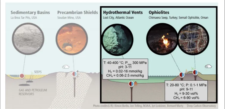
second order products of serpentinization reactions, which are the hydrothermal alteration of ultramafic rocks. As illustrated in
Figure 1, various proportions of H2 and CH4 are detected in
fluids from different serpentinizing systems over a wide range of pressure (P), temperature (T), and pH conditions, such as mid-oceanic ridges (Charlou et al., 2002; Proskurowski et al., 2006, 2008;Konn et al., 2009;Fouquet et al., 2013), or ophiolites (Chavagnac et al., 2013;Monnin et al., 2014;Etiope et al., 2018). These abiotic moieties have attracted much attention since they could serve as an energy source to sustain deep life and potentially contributed to its origin on Earth and elsewhere in the solar system (Sleep et al., 2004;Schulte et al., 2006;Oze and Sharma, 2007;Ehlmann et al., 2010;Russell et al., 2010;Hellevang et al., 2011;Zahnle et al., 2011; Glein et al., 2015;Holm et al., 2015;
Brazil, 2017;Etiope et al., 2018;Ménez et al., 2018).
H2 production during serpentinization results from the
oxidation of the ferrous component of ferromagnesian minerals (e.g., olivine, pyroxenes) coupled to the reduction of water (Thayer, 1966). In turn, H2 can reduce oxidized forms of
carbon into CH4and light hydrocarbons (HCs) via a Sabatier or
Fischer-Tropsch-type (FTT) reaction (Szatmari, 1989). Industrial reactions use CO as the carbon source under gaseous conditions with metal catalysts to overcome kinetics hindrance, either Ru-or Rh-based and Ni-based fRu-or Sabatier and FTT reactions, respectively. However, the main source of oxidized carbon in natural systems is CO2, bi-carbonate, or carbonate ions
depending on the pH, rather than CO, and reactions are likely to occur under aqueous conditions (McCollom, 2013). Consequently, the common use of Sabatier-type (R1) and FTT (R2) reactions among the geoscience community are:
4 H2+CO2= CH4+2 H2O (R1)
(3n + 1) H2+n CO2= CnH2n+2+2n H2O (R2)
The increased interest for these natural reactions over the last decades has led to a large number of thermodynamic modeling and experimental studies of serpentinization. Thermodynamic models using crustal conditions predict that H2concentration at
equilibrium with serpentinized peridotite increases with T and can reach hundreds of mM at optimum conditions (∼300◦
C) (Klein et al., 2009, 2013). This is close to the concentration expected near a reaction front, but an order of magnitude higher than those measured at oceanic vents (Andreani et al., 2013;
Fouquet et al., 2013). CH4 is favored relative to CO2 with
decreasing temperature and increasing H2 concentration, and
should be the dominant C-bearing component in hydrothermal fluids released from serpentinization at temperatures below 400◦
C (Shock, 1992,Zolotov and Shock, 1999, 2000;McCollom, 2013), similar to observations in natural fluids (Figure 1). In
experiments, the system tends toward equilibrium with time, but it is affected by kinetic effects that are related to a series of crucial parameters such as T, P, grain size, time, or fluid composition.
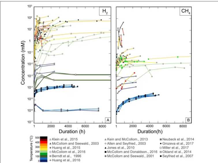
Figure 2shows a compilation of the H2and CH4concentrations
produced during experimental serpentinization from the original dataset (Huang et al., unpublished). These concentrations agree with our understanding of serpentinization kinetics, displaying a higher H2 concentration in higher T experiments (>200◦C)
than in low T ones (<100◦
C) (Figure 2A), and also overlap with natural concentrations. Nevertheless, a detailed examination of Figure 2A reveals some discrepancies between results for ranges of T that are not easily attributable to parameters that affect kinetics, and questions the optimum conditions for H2 production. The situation appears much more complex
and controversial when it comes to CH4 and HC production
(Figure 2B). Although some experimental concentrations agree well with measurements for high-temperature (HT) fluids, the experimental trend displays an increase of CH4as a function of T,
which is opposite to the decrease expected from thermodynamic models. Moreover, experiments using 13C labeled sources,
13CO
2, H13COOH, NaH13CO3, resulted in virtually no13CH4
production (roughly two orders of magnitude below 12CH4)
raising the issue of potential contamination by ubiquitous organic carbon in most experiments (McCollom and Seewald, 2001;
McCollom, 2003, 2016;Foustoukos and Seyfried, 2004;Fu et al., 2007; Ji et al., 2008;McCollom et al., 2010; Lazar et al., 2012, 2015; Grozeva et al., 2017). These experiments have fueled questions about whether the abiotic synthesis of CH4 during
serpentinization reactions actually occurs.
In order to feed the debate and achieve an unbiased reading of the available literature, we have built a comprehensive dataset of the experimental results of serpentinization available in the literature (Huang et al., unpublished), and, after dimensionality reduction, applied machine learning tools, a yet underused approach in geosciences. This approach provides an overview of the different conditions and protocols used so far, including the wide variety of experimental parameters that cannot be easily handled on regular plot (e.g., Figure 2). Finally, we discuss the variability of H2 and CH4 concentrations along with the
consistency of the global dataset.
DATA AND METHODS
Data Description
A large number of experiments have been conducted to study serpentinization, aiming at understand the abiotic production of H2, CH4, and other HCs during water–rock interactions (Berndt et al., 1996; Horita and Berndt, 1999; McCollom and Seewald, 2001, 2003;Allen and Seyfried, 2003;Foustoukos and Seyfried, 2004;Seewald et al., 2006; Fu et al., 2007, 2008; Seyfried et al., 2007; Ji et al., 2008; Dufaud et al., 2009; Jones et al., 2010;
McCollom et al., 2010, 2016; Marcaillou et al., 2011; Neubeck et al., 2011, 2014; Lafay et al., 2012; Lazar et al., 2012, 2015;
Klein and McCollom, 2013; Okland et al., 2014; Huang et al., 2015, 2016;Klein et al., 2015;McCollom, 2016;McCollom and Donaldson, 2016; Grozeva et al., 2017; Miller et al., 2017).
FIGURE 1 | Geologic settings of intense H2and CH4degassing on Earth. The red and blue colors reflect the biotic and abiotic contributions, respectively, of which
the relative fluxes are still under debate. The biotic production includes present-day microbial activity and thermogenic breakdown of organic matter from biological origin. The abiotic production results from radiolysis in Precambrian shields and serpentinization reactions at mid-ocean ridges or in ophiolites. Serpentinization settings are highlighted. (Credit: Josh Wood, modified with permission).
The most extensive dataset compiled so far is described in a companion data paper (Huang et al., unpublished). This dataset includes serpentinization experiments in which minerals are initially introduced as reactants, as well as experiments run without solid reactants. The latter correspond either to blank experiments—designed to evaluate unavoidable contaminations (e.g., background carbon or H2 production)—or to relevant
systems in which H2 levels would not be limited by mineral
dissolution and could reach higher values, such as experiments with formate as a source of H2and C.
The database (Huang et al., unpublished) indicates that the scientific community is mainly focused on two geological settings: ophiolites, characterized by low pressure (LP) and low temperature (LT) conditions (ambient or vapor saturation pressure, T< 100◦
C) and oceanic hydrothermal environments characterized by medium pressure (MP) to high pressure (HP) and HT conditions (30–300 MPa; 200–500◦
C). The highest pressures tested, at 350 MPa, are also relevant to shallow subduction environments where serpentinization occurs in the mantle wedge or fractured subducting lithosphere. There is a clear lack of data between 100 and 200◦
C, and between 50 and 300 MPa (Figure 3 and Supplementary Figure S1).
Various types of reactors were used to cover this large range of P-T conditions. For instance, gold cells in autoclave are common for experiments at HT (200–500◦
C) and HP (300 MPa) conditions (Huang et al., 2015, 2016; Lazar et al., 2015) while Parr type autoclaves, with or without flexible cells made of gold or titanium, are better suited for experiments
at HT (200–500◦
C) and MP (30–50 MPa) conditions (Berndt et al., 1996; Horita and Berndt, 1999; McCollom and Seewald, 2001, 2003;Allen and Seyfried, 2003;Foustoukos and Seyfried, 2004;Seewald et al., 2006; Fu et al., 2007, 2008; Seyfried et al., 2007; Ji et al., 2008; Dufaud et al., 2009; Jones et al., 2010;
McCollom et al., 2010, 2016; Marcaillou et al., 2011; Lafay et al., 2012; Lazar et al., 2012; Klein and McCollom, 2013;
Klein et al., 2015; McCollom, 2016; Grozeva et al., 2017). Comparably, borosilicate glass bottles were preferred for LT and LP experimental conditions (Neubeck et al., 2011, 2014;
Okland et al., 2014; McCollom and Donaldson, 2016; Miller et al., 2017). Figure 3 is a swarm plot showing the number of data points in green of a given value for a series of selected parameters. The gray box represents the 25–75th percentile and the gray line is the median value. The gray lines outside the box represent the minimum and maximum values, with the exception of outliers. P, T, and initial/final pH of the fluid follow a bimodal distribution that mimics the natural conditions illustrated in
Figure 1. Addition of NaCl or NaHCO3salts, presence of catalyst,
and gold capsules are the most frequent features in the dataset, used in more than 50% of experiments. This indicates that inorganic carbon in experiments is most often introduced as NaHCO3 salt, and that the most classical reactors are made of
gold. Other dataset features are highly variable, for example, all experiments have their own starting materials (e.g., mineral assemblages, fluid compositions), sample volumes that range from 0.05 to 180 mL, and experimental run durations from hours to a year.
feart-08-00209 June 12, 2020 Time: 19:58 # 4
Barbier et al. Network Analysis Abiotic Methane
FIGURE 2 | Summary of H2(A) and CH4(B) concentrations produced as a function of time and temperature during serpentinization experiments, in which duration
can reach ca. 11 months. Concentrations span over eight orders of magnitude from nanomoles to hundreds of millimoles.
FIGURE 3 | (A) Presentation of the general attributes of a swarm plot that helps to visualize the distribution of a selected data feature (green dots), e.g., temperature, H2, CH4, and related boxplots. (B) Swarm plots of the distribution of data according to experimental parameters and results analyzed in this contribution. The x-axis
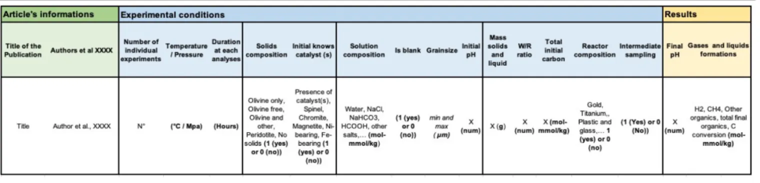
TABLE 1 | Description of the working dataset modified from Huang et al. (unpublished) organized in three major sections: article’s information (green), experimental conditions (blue), and results (yellow).
Sub sections and summary of contents are also displayed with examples of value, unit when appropriate, character (0 or 1).
The complete dataset (Huang et al., unpublished) includes more than 100 parameters. Each column represents a feature, such as an experimental parameter, reactant, or product, and each row is a measurement. Some of the 100 features of the complete dataset are too sparse to allow running data analysis algorithms directly. Hence, in the present study, we performed dimensionality reduction by removing the less variable parameters and combined some features to increase data density within 37 features in a working dataset (Table 1). Hereafter, we will refer to the header of the column that is an explicit shortcut for its content. For example, the “Other_organics” feature sums all organic products except CH4; the “Fe_bearing” feature combines all Fe-bearing solids
(synthetic or natural) added to the system (e.g., FeO, hematite, sulfides) except olivine and magnetite, which are considered as independent parameters. Some experiments include multiple samplings as a function of time and had more than one measurement (as shown in Figure 2); in these cases, only the final measurements were kept for the analysis in order to prevent overweighting those experiments in the analysis. Hence, the final working dataset includes 158 measurements in total, which result from experimental runs with different durations.
Pearson Correlation Coefficient Matrix
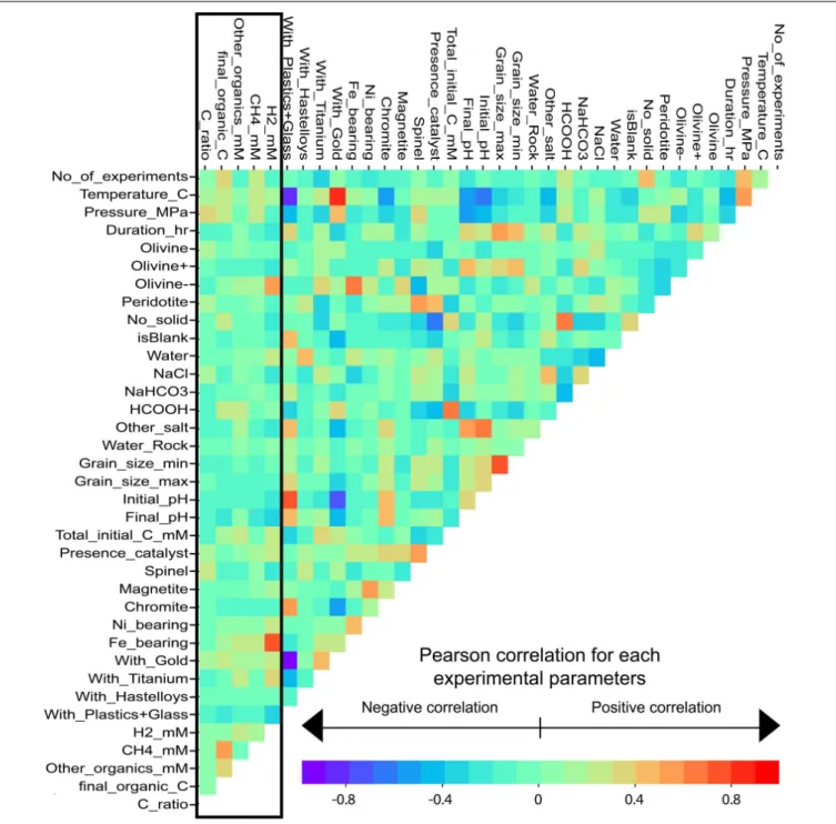
The Pearson correlation coefficient is a value between -1 and 1 that indicates the extent of linear correlation between two variables. A coefficient of -1 or 1 means the two variables are in perfect negative or positive correlation respectively, with 0 indicating no correlation. Details of how the coefficient is calculated can be found in Pearson (1895) and Lee Rodgers and Alan Nice Wander (1988). The pairwise Pearson correlation coefficient matrix for our final dataset is calculated and displayed in Figure 4.
It is worth noting that some parameters are dependent and led to some of the strongest correlation, e.g., between “CH4,” “Other_organics,” and “Total_final_organics,” the latter
being the sum of the formers. Another example is “Spinel,” which correlates with “Peridotite” and “Presence_catalyst” because peridotite is partly composed of spinel and spinel is a common catalyst of some reactions. Conversely, “Magnetite,” which was separated from the “Fe-bearing”
and “Spinel” lists, does not correlate with “Fe-bearing” and “Spinel.”
The experimental protocol also induced some strong correlations. For instance, temperature is strongly positively correlated with the parameter, “With_Gold,” and negatively correlated with the parameter, “With_Plastics+Glass,” classically used for HT and LT experiments, respectively. Similarly, the use of formate, “HCOOH,” as a source of carbon and H2
is strongly correlated to the highest levels of initial carbon, “Total_Initial_C_mM,” which are used in the gold reactors (“With_Gold”) predominantly in experiments that did not include mineral phases (“No_solid”).
The black box (Figure 4) highlights the correlations of interest, i.e., between all parameters, H2, and carbon products. It shows
the lack of strong correlations that prevent the interpretation of the database using conventional wisdom. These relationships are presented and discussed in Section “Results and Discussion,” with the help of network analysis.
Network Analysis
Network analysis is a collection of analytical and visualization methods that have been employed to study complex systems in various fields of science and technology. For example, in biology, it has been applied to the study of ecosystem diversity ( Banda-R et al., 2016), proteomics and protein–protein interactions (Amitai et al., 2004;Harel et al., 2015), evolution (Vilhena et al., 2013), and mass extinction events in Earth’s history (Muscente et al., 2018, 2019). In urban planning, networks have been used to model power grids (Pagani and Aiello, 2013), roads (Dong and Pentland, 2009), and water supply systems (Geem, 2006) as well as communications infrastructure (Hansen and Smith, 2014). Networks of people have also featured prominently in the study of social media, the spread of infectious diseases, the structure of criminal organizations, and connections among research collaborators (Otte and Rousseau, 2002;Abraham et al., 2010;Eslick, 2012;Scott and Carrington, 2015).
The power of network analysis arises mainly from its capability of representing and visualizing large sets of highly dimensional data and exposing the complex relationships amongst them. Entities are represented by nodes (vertices) and are connected by edges (links) that illustrate the relationship
feart-08-00209 June 12, 2020 Time: 19:58 # 6
Barbier et al. Network Analysis Abiotic Methane
FIGURE 4 | Pearson correlation coefficient matrix between all parameters analyzed in the dataset. Warm and cold colors show positive and negative correlation, respectively. The black rectangle across the first five columns highlights the five important experimental products.
between entities. The visual attributes of the nodes such as shape, color, or radius, and of edges such as weight (line thickness), can be mapped to values resulting in a dynamic and more expressive network diagram. Visual inspection of the diagram with some perturbation of the parameters is a powerful tool for revealing potentially unseen patterns and characteristics in the data. A number of quantitative analytical techniques can be applied to the network in order
to study and quantify the significance of these patterns and behaviors.
In this methodology, the nodes refer to each experiment within the dataset, and edges represent the similarity between different experiments. Therefore, nodes that cluster together have short edges, and represent similar experiments. At the end of the analysis, a cluster of nodes then becomes a community of similar experiments. The
method to calculate similarity scores is explained in the following section.
Cosine Similarity Matrix
The network is built from a pre-calculated cosine similarity matrix (Janbandhu and Karhade, 2015). Each experimental measurement can be treated as a 35-dimension numeric vector (37 experimental features minus two article information features), and the pairwise cosine similarity score is calculated between each vector. The cosine similarity scores between two experimental features represent the combined effect of all parameters and vary between −1 and 1.
In the working dataset, 0 stands for no and 1 for yes, for categorical values. Numerical values such as temperature, pressure, or durations were normalized between 0 and 1 to avoid biases due to different value ranges. We then used the similarity scores as the edge weights of the networks. Since we consider just serpentinization experiments, many studies have some parameters in common, which results in a fully connected network with varying edge weights. Even though a fully connected network contains abundant information and potential insights, we choose to optimize the efficiency of the community detection algorithms by choosing a threshold to eliminate edges with low importance. For this purpose, we ran experiments by eliminating edges with low similarity scores and testing their effects on the results of the community detection algorithms.
Fruchterman–Reingold Force-Directed Networks
The Fruchterman–Reingold force-directed graph algorithm (Fruchterman and Reingold, 1991) simulates attractive and repulsive forces between the nodes, similar to those of molecular or planetary simulations, while attempting to find a minimum energy state for the network layout. It is based on two general principles: (1) nodes connected by an edge should be drawn near each other and (2) nodes should not overlap. To compute the layout, the method iteratively adds nodes to the diagram while recalculating the attractive and repulsive forces and displacing existing nodes accordingly. As such, we do not control the lengths of the edges or the final positions of the nodes, which are determined when the system reaches equilibrium. In this study, we use a python package calledNetworkx (v. 2.3) (Hagberg et al., 2008) to build the network. The 3D network structure is fixed by this algorithm, but its 2D projection can change at different angles randomly, meaning that every time when we run the code, the 2D project will change. For any algorithm involving randomization, a seed can be used to make the algorithm produce consistent results. We tested a set of seeds from 0 to 200 and found that seed 103 gives the clearest and most informative layout for our data. If the reader wants to reproduce our results, please use the same seed number as ours.
Louvain Community Detection Algorithm
The Louvain community detection algorithm (Blondel et al., 2008) attempts to find community structure in a network through multi-level modularity optimization. Initially, each node is assigned to its own community. At each step, nodes are
reassigned to the communities with which they achieve the highest contribution to modularity. When no more nodes can be reassigned, the process is applied again to the merged communities and is stopped when there is only a single vertex remaining or modularity cannot be further improved. The algorithm in this paper is implemented using a package called python-louvain1.
RESULTS AND DISCUSSION
Detection of Four Communities of
Experiments: A Snapshot of the
Literature
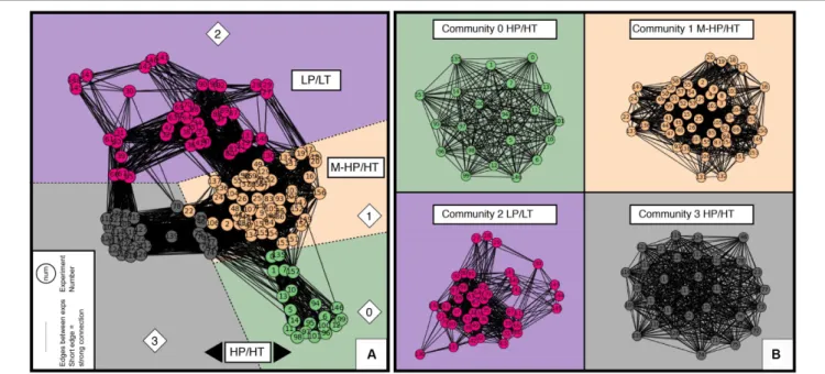
The Pearson similarity matrix (Figure 4) built from our dataset revealed no clear trend between experimental parameters and reaction products. It mostly identifies a couple of strong and inevitable correlations between some experimental parameters, such as the use of gold cells for HT experiments (see section “Pearson Correlation Coefficient Matrix”). However, it confirmed that (despite some trends on the kinetic curves that could already be drawn using the complete database; Figure 2), data discrepancies cannot be easily interpreted using conventional wisdom. We used the parameters reported from each experiment in our dataset to build a cosine similarity matrix, and then constructed a network (see section “Data and Methods”) with a layout defined by Fruchterman–Reingold force-directed graph algorithm. Four communities were detected using the Louvain community detection algorithm, as colored distinctively in Figure 5A, and plotted individually in Figure 5B. These experimental communities present overall similarity among different experiments when taking into account all experimental features, including starting materials, reactants, reactors, fluids, reaction products, and potential catalysts. Hence, they provide a full “picture” of the available literature, i.e., the conditions that have been explored to date and the degree of similarity or dissimilarity of the results. For ease of comparison, the network diagrams presented in Figure 5 follow the same color chart and layout throughout the manuscript.
The cosine similarity threshold and the initial node have been tested before ending up with these four experimental communities. Supplementary Figure S2 shows that by successively removing the weakest 10, 30, 50, and 70% of the edge connections, the communities detected by Louvain algorithm are quite similar. We therefore infer that these communities are robust and represent real trends in the data. The number of communities detected is always four, and communities 0, 1, and 3 virtually stayed the same. When we remove the weakest 70 % of edge connections, nodes 143, 144, and 145 in community 3 moved into community 2.
Our analysis enabled us to find the optimum threshold (0.39) where the community detection algorithms produce very similar results to the densely connected networks, while increasing the efficiency of the network. This approach assisted in identifying the important edges in the network structure. Depending on
feart-08-00209 June 12, 2020 Time: 19:58 # 8
Barbier et al. Network Analysis Abiotic Methane
FIGURE 5 | Networks built with the cosine similarity matrix calculated from the dataset, with the four detected communities that are a snapshot of the conditions tested so far and their usual experimental protocols (community 0: HP/HT using HCOOH as a source of C and H2, community 1: M-HP/HT, community 2: LP/LT,
community 3: HP/HT with C_ratio> 1) (see Figures 6, 7). (A) The full network. Each filled circle (node) represents an experiment, which number is included and allows to back track the corresponding experiment in the database. The shorter the link (edge) between two circles, the higher the correlation between the experiments. (B) The four separate community networks. Communities have been arbitrarily color coded as a guide for the eyes, which remained the same in all figures—green, brown, purple, and gray, for communities 0, 1, 2, and 3, respectively.
the initial node chosen by the algorithm, the number of detected communities was dominantly four but could increase to five occasionally. The initial node is chosen randomly by the algorithm, and the random state can be set with a random seed. As explained in Section ““Fruchterman–Reingold Force-Directed Networks,” if you want to reproduce the layout of our plots, please use a seed of 29. As the random seed varied, community 0 always remained the same, but a few nodes on the edges of communities 1 and 2 (e.g., node 143, 144.), and 1 and 3 (e.g., node 22, 46, 106) would change.
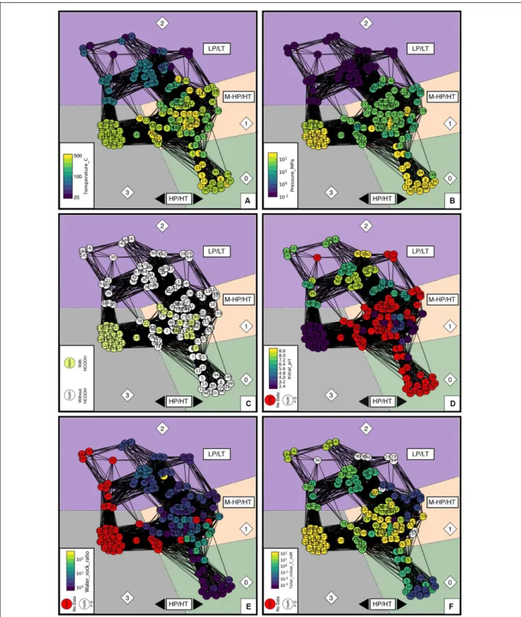
In order to identify the main features that control the separation into the four communities identified with Louvain algorithm, we colored the nodes of the network as a function of the value of each experimental parameter. For parameters with binary values, white and lemon colors were used for 0 and 1, respectively. Red stands for unreported values. Selected plots are displayed in Figure 6; others are available in Supplementary
Figure S3. This data analysis highlights the primary control of temperature (T) and pressure (P) on the experimental communities (Figures 6A,B), akin to natural end-member conditions (Figure 1). Community 2 clearly corresponds to LP/LT experiments at ambient P and T below 100◦
C, while the other communities encompass experiments run at higher P and T. Community 1 differs from communities 0 and 3 because of pressure and covers MP range between 10 and 100 MPa. Community 3 differs from community 0 and others because it contains experiments that exclusively used the decomposition of formic acid HCOOH as a source of H2 and CO2 and buffered
the initial pH to the lowest values reported in the literature
(Figures 6C,D). Community 3 also lacks information on the water-to-rock ratio since neither a solid phase (Figure 6E and
Supplementary Figure S3A), nor NaCl was added to the fluid
(Supplementary Figure S3B), distinguishing it from almost all other experiments. It is worth noting that except for experiments performed with HCOOH, initial pH values are rarely reported in experiments within communities 0 and 1, and are most likely close to neutral or slightly alkaline considering the presence of NaCl with or without NaHCO3, respectively. Visualization
of community 2 shows that LP/LT experiments have also been run at neutral to basic conditions to mimic outflow fluid composition in ophiolitic settings. Hence, experimental results of community 3 cannot be directly compared to the others and will be plotted in the following graphs for informative purposes only. Detailed examination of the communities’ characteristics highlights the lack of experiments under initial acidic conditions that are supposed to be the most favorable for olivine dissolution (Oelkers, 1999;Kaszuba et al., 2013). This might be due to the fact that natural serpentinizing systems are not expected to be acidic at a temperature of or below 300◦
C. However, reaction with acidic HT hydrothermal fluids such as those escaping from peridotite-hosted hydrothermal vents at slow-spreading ridges can occur (Fouquet et al., 2013). Finally, analysis of the communities shows that the initial fluid composition is a feature that has never been explored so far, especially in HT experiments.
When looking at individual communities (Figure 5B and
Supplementary Figure S4), experiments are also well grouped into clusters of LP/LT, MP/HT, and HP/HT conditions, even if P and T only partially characterize the communities. Communities
FIGURE 6 | Values of the parameters that dominantly control the distribution of the data in four different communities of experiments: (A) temperature in◦C; (B)
pressure in MPa; (C) presence or absence of formic acid in the starting aqueous solution, with or without HCOOH; (D) pH of the starting aqueous solution (Initial_pH); (E) relative amount of water and rock (Water_rock_ratio); and (F) the total initial carbon concentration in the starting aqueous solution by adding up all carbon species (Total_initial_carbon_mM). All red filled circles indicate that the value of the parameter is missing in the original article that presents the experiment.
feart-08-00209 June 12, 2020 Time: 19:58 # 10
Barbier et al. Network Analysis Abiotic Methane
1 and 3 contain the highest number of nodes while community 0 is the smallest one, illustrating the limited number of experiments run at the pressure of hundreds of MPa. Communities 0, 1, and 3 form round layouts, whereas the layout of community 2 is irregular. Considering the layouts are defined by the force directed algorithm, this analysis indicates that the diversity of experimental parameters, notably fluid composition, is generally much larger in LP/LT experiments (community 2) than in others. For example, this is visible when looking at the variety of initial pH values, “other_salts” (e.g., MgCl2, CaCl2), or
water-rock ratio tested under ambient pressure and temperature below 100◦
C (LP/LT).
H
2, CH
4, and Hydrocarbon Production
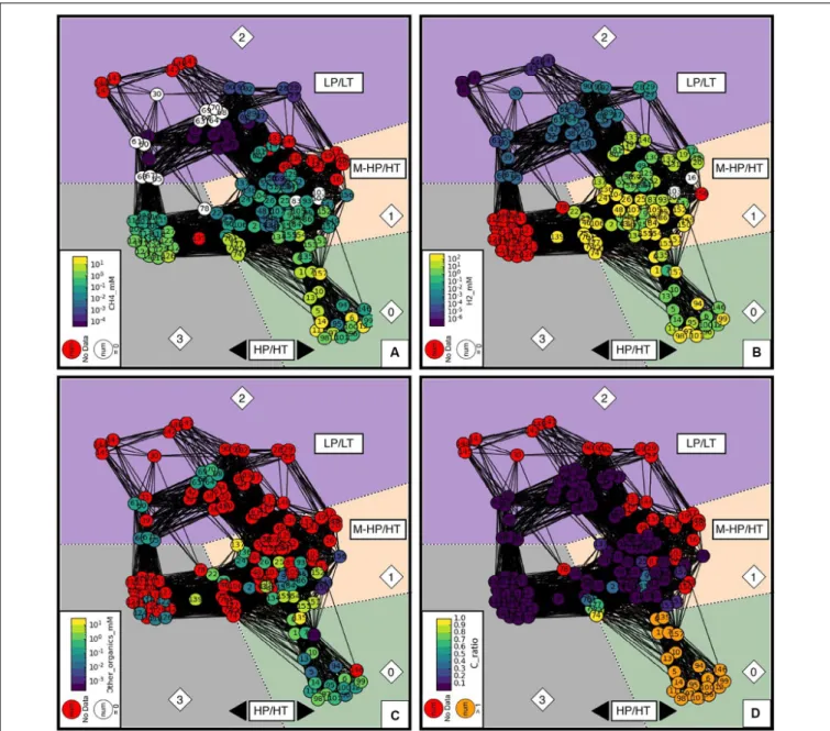
Figure 7shows the distribution of the concentrations of gaseous H2, CH4, and other organics together with the carbon ratio
(“C_ratio”) among the four communities. The C_ratio is the ratio between the carbon initially introduced in the system and the final measured one, according to the available information. This cannot take into account the potential carbon contamination of reactants that has never been quantified by the authors of the publications analyzed in the database. The distribution of H2
concentrations across communities is bimodal, spans eight orders of magnitude, and correlates with temperature (LT versus HT) but not pressure (Figure 7A) with the exception of community 3, whose experimental production of H2was not reported. CH4
concentration spans five orders of magnitude and correlates with both T and P (Figure 7B); production is lower at LP/LT (community 2) than at HT (communities 1 and 3), and the highest concentrations are clustered in community 0 at HP. Community 0 is also characterized by “C_ratio” values higher than one (Figure 7D), which are unrealistic and necessitate that an unidentified source of carbon was present in the system, hence indicating contamination issues with the samples. It may also be responsible for the occurrence of other organic products (“Other_organics”), which systematically occur in community 0 (Figure 7C) and are occasionally observed in the others. Therefore, we will not discuss the results of community 0 further.
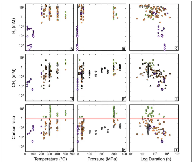
Figure 8 further illustrates the evolution of H2 and CH4
concentration as a function of P and T together with values from 13C-labeled and blank experiments. As our dataset only considers the last sampling point of each experimental set (see section “Data Description”), the experimental duration varies from one data point to another. Hence, we also plot H2 and
CH4 concentration as a function of duration (Figure 8C) to
check whether the variability observed at a given P or T does not simply result from experimental duration (reaction kinetics).
Figure 8confirms the overall trends depicted on Figure 2 (regular kinetic curves using the non-reduced database) for both H2and
CH4 distribution and better highlights the strong variability of
concentrations for given P-T conditions. The lack of consistency of the whole database is confirmed by the absence of correlation between gas concentrations and duration when observing all final experimental points from different experiments (Figures 8C,F). It is worth noting that blank experiments are frequently reported at LP/LT, while none are available at higher T to establish background levels of H2 and CH4 under those conditions.
Experiments starting with 13C labeled sources have been used instead to test carbon contamination issue in a limited number of experiments (triangle symbols in Figure 8), but background levels of H2remain unknown to date.
The evolution of H2 concentration as a function of P and
T (Figures 8A,B) also highlights two regimes of reaction, at LP/LT below 100◦
C in the MPa range, and at MP– HP/HT above 200◦
C. In the LP/LT regime (community 2), H2 concentration is low, between 10−1 and 10−3 mM, and
blanks indicate that concentrations below micromolar are not significant. In the MP–HP/HT regime (communities 0, 1, and 3), H2 concentrations can almost reach molar concentrations.
HCOOH-bearing experiments (community 3) always have the highest values reported. This is expected because in these cases H2 comes from the decomposition of HCOOH that was
introduced at high concentration (10–100 mM) in the starting fluid. In the other groups where H2results from redox reaction
with iron-bearing phases, H2 concentration is highly variable
and no sweet spot for H2 production could be identified,
hence preventing the description of a trend with either T or P (Figure 7). This does not correlate with serpentinization kinetics deduced from solid phase transformation (olivine-to-serpentine transformation, Martin and Fyfe, 1970; Malvoisin et al., 2012; McCollom et al., 2016). Indeed, serpentinization kinetics classically display a bell curve with a maximum at ∼250–300◦
C that is not observed in the current H2dataset. H2
concentrations are neither correlated to duration nor to grain size (Figure 4). Available data on initial pH (Figure 6D) are too scarce to be conclusive. Rather, Figure 4 shows that H2
concentrations display strong positive correlation with “Olivine-” (i.e., olivine-free run) and “Fe_bearing“Olivine-” features, which are highly correlated to each other as well. This suggests that the highest levels of H2 are reached with a source of Fe
(0 or II) other than olivine, i.e., derived from Fe-bearing species such as Fe-bearing salts, oxides, or alloys. Olivine, whose iron content is lower and whose release in the fluid is controlled by dissolution kinetics, appears less efficient at producing H2 than the other iron-rich compounds. However,
this does not explain the variability among serpentinization experiments [i.e., the olivine-bearing experiments (“Olivine” and “Olivine+”) that dominate the database (e.g., Figure 2)]. It is worth noting that H2also positively correlates with the presence
of catalysts “Presence_catalyst” (Figure 4), whose occurrence is widely distributed among all communities (Figures 10A–D) suggesting either a catalytic or a reactive role of these phases on the production of H2(see section “Effect of Accessory Solid
Phases” for details).
In order to produce abiotic methane, assuming that it forms by an FTT reaction, an oxidized form of carbon is often added to the starting fluid. The CH4 concentration is then
measured (Figure 2B) at the end of experiments. The evolution of CH4 evolution as a function of P and T (Figures 8D,E)
first shows that CH4 concentrations are one to two orders of
magnitude below those of H2(Figure 9A). Figures 9B–D show
that CH4concentrations are also well below the concentrations
of the oxidized carbon sources deliberately introduced in experiments, except for community 0 which was removed from
FIGURE 7 | Networks of concentrations of: (A) CH4, (B) H2, and (C) other organic species. The heatmap color from cold to warm corresponds to low to high
concentrations. Red nodes refer to experiments that did not report relevant concentrations. Experiments labeled in white have concentrations below detection limits, which are set to 0 in the database. (D) C_ratio - total final carbon divided by total initial carbon. Theoretically, C_ratio should be between 0 and 1. Dark purple nodes are experiments that did not include or report initial carbon concentrations (set to 0 by convention). Red nodes refer again to final carbon concentrations not reported in the original literature. The orange nodes, mainly in community 0, are experiments reports more final carbon than initial carbon, i.e., C_ratio higher than 1. This suggests that those experiments might have undocumented contamination issues.
discussion because of an unrealistic “C_ratio” (Figure 7D). First, this indicates that the low CH4 concentrations do not result
from limited reactant availability for reaction R1. Second, it suggests that CH4 formation by reduction of oxidized carbon
forms, if possible, is not efficient and far from equilibrium. Only LP/LT experiments displaying the lowest values of methane concentration achieve values close to expected CH4
concentrations (Figure 9A). These low methane concentrations, near micromolar level, are still above those of blank experiments run at similar conditions. At high T, 13C-labeled experiments
report undetectable to micromolar levels of 13CH
4, whether
catalysts are present or not (see section “Effect of Accessory Solid Phases”). These concentrations are well below the CH4
concentration measured in all other experiments (Figures 8D–
F, 9B–D). Assuming that the use of a heavy carbon source in
13C-labeled experiments does not have a kinetic effect on carbon
reduction reactions, these results indicate that abiotic CH4 has
never been formed at a significant level during serpentinization experiments. As such a strong statement rules out most of—if not all of—the available literature we further investigated the present
feart-08-00209 June 12, 2020 Time: 19:58 # 12
Barbier et al. Network Analysis Abiotic Methane
FIGURE 8 | Concentrations of H2(A–C), CH4(D–F), and carbon conversion (G–I) displayed as a function of temperature (A,D,G), pressure (B,E,H), and experiment
duration (C,F,I). Diamond symbols correspond to “blank experiments” run without minerals in the experimental load. Thick triangle symbols in (D–F) highlight13CH 4
concentration while thick circles show the corresponding total CH4also including12CH4. In (G,H), the red line corresponds to a carbon ratio value of 1, beyond
which is suspected to be contaminated. Color coding consistent with Figure 5.
database to discuss this hypothesis (see section “Contamination Issues”) and investigated the consistency of the available data for actual CH4production by an FFT process.
The dataset shows that CH4 concentrations display a
logarithmic increase with T between ambient T and 500◦
C (Figure 8D) and they do not show any dependence on pressure above 30 MPa. The increase of CH4 concentration with T is
also well highlighted by the 13C-labeled experiments, despite much lower13CH
4concentrations. The strong variability of CH4
concentrations among experiments from the largest community (community 1) precludes any further correlation between CH4
and pressure. Figure 8F highlights that duration does not account for the variability of CH4 concentrations in experiments at
given P-T conditions. The same holds for “grain_size,” which is uncorrelated with CH4concentrations (Figure 4).
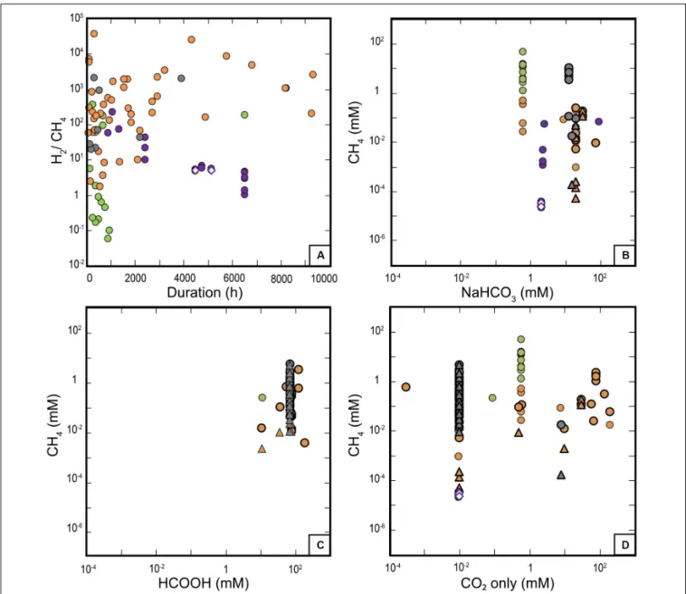
McCollom et al. (2010)suggested that the nature of initial carbon source may affect the system reactivity, and they showed that dissolved CO and HCOOH carbon sources are more effective at abiotic organic synthesis than CO2. We test this hypothesis
by comparing the CH4 concentrations reached for the different
types of carbon source ((bi-)carbonate salts, HCOOH, or CO2)
(Figures 9B–D). This selection of carbon sources is not the choice of the authors, it simply reflects the C-sources reported in the publications. HCOOH-bearing experiments (mainly community 3—all run at similar T conditions), in which high amounts of HCOOH have been added (10–100 mM), produced the highest
FIGURE 9 | (A) H2/CH4ratio as a function of time. CH4concentration as a function of the initial carbon sources in experiments (bi-)carbonate salts (B), HCOOH (C),
and CO2(D). Thick triangles and circles correspond to labeled13CH4and total methane, respectively. Color coding consistent with Figure 5.
CH4 concentrations (∼10 mM) at HP (Figures 8D,E, 9C),
excluding data from community 0 because of contamination issues. Such experiments, in which olivine is mostly absent and HCOOH decomposes to H2, CO2 (±CO) at HT, are reported
here for comparison but are not representative of the actual serpentinization process investigated so far in experiments. Experiments of community 2 at LP/LT have only used NaHCO3
at one concentration and show variable CH4 production. It
appears that the most comprehensive dataset for this discussion is provided by the experiments in community 1 at MP–HP/HT. In community 1, CH4concentrations display an overall correlation
with CO2 content, which is also evidenced in 13C-labeled
experiments for lower CH4 concentrations. Such a correlation
is not observed with initial NaHCO3 concentrations whose
variation range is too limited. This precludes the comparison between the reactivity of carbonate/bicarbonate ions versus CO2.
The above observations show that despite considerable efforts, the available experimental dataset remains incomplete and limits the analysis. Nevertheless, results deeply question the potential of these carbon sources to efficiently react with the H2 derived
from serpentinization, and suggest a strong inhibition of R1 under those conditions, even with high reactant concentrations. In addition, the increase of CH4as a function of T (Figure 8D)
does not follow thermodynamic predictions and rather indicates a kinetic or a thermal control of experimental CH4production,
whatever the reaction is. The only plausible trajectory toward equilibrium is observed for LP/LT experiments (community 2,
feart-08-00209 June 12, 2020 Time: 19:58 # 14
Barbier et al. Network Analysis Abiotic Methane
phase in most of these experiments run into incubation flasks, i.e., in conditions closer to those ideal for reactions R1 and R2. The potential importance of a gaseous phase that could be mandatory for CH4 production was already raised by some
authors and deserves further investigation (Etiope et al., 2011;
McCollom, 2013).
Data on the production of organic products other than methane are very sparse and were combined in the dataset into a feature called “Other_organics” (Figure 7C) that dominantly includes small organic molecules (<0.1 mM) measured in either the liquid phase at LP/LT (organic acids, community 2) or the gas phase at MP/HT (HCs, communities 1 and 3). These sparse data do not show any obvious correlation with CH4, as possibly
expected from reaction R2 (Figures 4, 7C). Figure 4 rather points to a positive correlation between “Other_organics” and “Total_inital_C” that is potentially true for the whole P-T range since “Other_organics” (mainly in the form of organic acids) were also detected at LP/LT conditions in the aqueous phase while CH4was not.
Effect of Accessory Solid Phases
Metal-bearing catalysts are critical to the industrial production of H2 or CH4 in gaseous phase. Notably they are critical for
(R1) and (R2) to overcome the first step of CO2 reduction
to CO by the water-gas shift reaction. The lack of data on CO occurrence and concentration in hydrothermal experiments focusing on serpentinization does not allow either decomposing reaction mechanisms or discussing the potential role of CO as an intermediate phase, which has been examined by a previous experimental study (Seewald et al., 2006). In addition, under aqueous conditions, the catalytic phases can be more reactive and propitious to alteration and consequently act either as real catalysts (do not react but accelerate the reaction) or as reactants whose transformation directly produces H2 (e.g., alloy) or
facilitates olivine dissolution, such as aluminum (Andreani et al., 2013). Addition of any material in a reactor also induces potential introduction of carbon contamination that could contribute to gas production.
To distinguish the role of potential catalysts, an in-depth characterization of the solid surfaces before and after experiment is mandatory. Unfortunately, this step has not been done in the large majority of experiments, hence preventing any inference. This also precludes the potential identification of precipitated carbonaceous phases among solids (Milesi et al., 2015; Andreani and Ménez, 2019). Here we take advantage of the dataset to discuss potential correlation between the concentration of reaction products such as H2, CH4, or the
other organics, and the presence or absence of potential catalysts in experiments for guiding future studies. The list of potential catalysts includes those introduced in the experiments as solids, natural or synthetic, such as Cr-spinel, magnetite, chromite, Ni- or Fe-bearing minerals or alloys. It also includes those produced by the serpentinization reaction such as magnetite or spinel, that have a recognized significant effect on the reaction. For example, spinel has been shown to improve H2
production at LP/LT (Mayhew et al., 2013). We also do not underestimate the potential catalytic role of the constitutive
materials of the reactor vessels commonly made of Au, Ti of HastelloyTM (a Ni/Fe-bearing alloy), whose catalytic properties
have been demonstrated for some other reactions notably in aqueous systems, for example, CO2 reduction to CO (Chen et al., 2012), reforming reactions (Van Haasterecht et al., 2014), H2 production (Michiels et al., 2018;Fowler et al., 2019), and
HCOOH dehydrogenation (Brunet and Lanson, 2019). Despite such evidence, especially for Au and Ti which are the most used for studying serpentinization reactions, reactor vessels are classically considered as inert for geochemical experiments dedicated at understanding the potential of serpentinization to produce abiotic H2, CH4, and light HC.
In the previous section, we highlighted the positive correlations between H2 and the presence of potential
metal catalysts (“Presence_catalysts”). A more detailed examination of Figure 4 shows a positive correlation between H2
production and the following catalysts, in decreasing order: “Fe-bearing”> “Titanium” > “Au” ∼ “Ni-bearing” > “magnetite.” “Chromite” and “Hastelloy” have no correlation and “Spinel” a potentially negative one with H2. The case of titanium reactors
is well known as Ti-reactors have to be pre-oxidized prior to hydrothermal experiments in order to avoid H2 production
from Ti oxidation (Seewald et al., 2006) and we reasonably assume that this step was run before experiments. Hastelloy, gold, or Ti do not have any recognized catalytic properties for H2 production or CH4 formation, and the strong correlation
between H2 concentrations and gold or titanium could also
well be due to the fact that H2 production is intrinsically
more efficient at MP-HP/HT in hydrothermal reactors that are systematically made of gold and titanium. Hence, it is not yet possible to disentangle between P-T and catalytic effects here. Figure 10 shows the concentrations of H2 as a
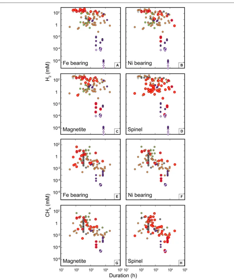
function of experimental duration for experiments run with the catalysts usually considered as the most optimal, i.e., omitting reactor metals and spinel, the latter displaying a slight negative correlation with H2. Figure 10 fits well with the ordering
of potential catalysts previously identified on Figure 4 (“Fe-bearing”> “Ni-bearing” > “magnetite”). Irrespective of the run duration or the community, the addition of “Fe-bearing” phases that encompass both Fe(II) and Fe(III) compounds appears to be the most efficient and leads to the highest production of H2 (Figure 10A). A strong contribution of Fe(II) oxidation is
expected in most cases but there may be underappreciated effects of Fe(III)-bearing phases yet to be explored in future works. H2
synthesis is also clearly enhanced by the presence of Ni-bearing phases at MP/HT conditions (community 1) while magnetite seems to be efficient for both LP/LT (community 2) and MP/HT conditions (community 1). As for “Fe-bearing” phases, oxidation of Fe(II) in magnetite and of Ni or reduced sulfur in Ni-bearing phases such as alloys or sulfides may intrinsically produce more H2 without a true catalytic effect occurring. Indeed, moderate
amounts of Ni metal particles have recently been identified as catalysts of FeO oxidation under hydrothermal conditions (Michiels et al., 2018) and this effect may be extrapolated to Fe-bearing minerals such as olivine (Brunet, 2019). Conversely, H2concentrations in spinel-bearing experiments cover the whole
FIGURE 10 | Potential catalytic effects on the formation of H2and CH4. Concentrations of H2(A–D) and CH4(E–H) are plotted against run durations. Diamond
symbols correspond to experiments without initial mineral phases, and red thick circles highlight the experiments with relevant catalyst reactants. (A) “Fe-bearing” ones include metallic iron, hematite, Ni-Fe alloys, FeS, FeO except magnetite; (B) “Ni-bearing” ones include NiS, Ni-Fe alloys; (C) “Magnetite” corresponds to experiments with magnetite; (D) “Spinel” corresponds to experiments with spinel or spinel-bearing peridotite. Color coding consistent with Figure 5.
feart-08-00209 June 12, 2020 Time: 19:58 # 16
Barbier et al. Network Analysis Abiotic Methane
(all communities) and always lie below the maximum values observed, which explains the negative correlation observed in
Figure 4. Hence, spinel does not appear as a good candidate for catalyzing H2production under those conditions. The effect
on H2 production of those different phases often introduced
in experiments contributes to the variability of concentrations observed for similar thermodynamic conditions, whatever the mechanisms behind.
The correlation between the presence of potential catalysts “Presence_catalysts” and CH4concentration is much lower than
for H2, and simply zero with “other organics” (Figure 4).
Potential effects of the different catalyst candidates appear in the following decreasing order for CH4: “Fe-bearing”> “Au” >
“Ni-bearing” ∼ “Magnetite” ∼ “spinel,” while “Ti,” “Hastelloy,” or “Chromite” have no correlation with CH4 concentration
(Figure 4). As for H2, we will not consider metals constitutive
of reactors any further and rather focus on the effects of “Fe-bearing,” “Ni-“Fe-bearing,” “Magnetite,” and “Spinel” (Figure 10). Spinel correlates more positively with the “Carbon _ratio” (Figure 4) than with CH4and is not explained by any correlations
with “Other_organics” or “Total_final_carbon.” This is probably due to the fact that the highest values of “Carbon_ratio” are obtained in the experiments of community 0. These experiments were run with spinel-bearing peridotites as reactants and produced such a large amount of methane at HT that they reached an unrealistic carbon ratio beyond 1, indicative of contamination as aforementioned. Contrary to H2 catalysis,
the weak correlations noticed in Figure 4 are hardly visible in Figure 10 for CH4 that does seem affected by any of the
selected potential catalytic phases, whatever the community. This questions some previous results that have highlighted the potential role of similar catalysts to explain the high CH4
concentration obtained in their experiments. Our analysis of the dataset compiled from the literature is again in better agreement with the results of13C-labeled experiments that did not detect any significant 13CH4 production despite the presence of potential
catalytic phases (McCollom et al., 2010;Grozeva et al., 2017).
Contamination Issues
The previous sections have shown that H2 is systematically
and significantly formed in experiments, indicating that its production during serpentinization is well established. This is apparent even at LP/LT, despite the general lack of blank experiments required to estimate background levels at these conditions. Catalytic effects and reactive Fe-bearing phases other than olivine contribute to the observed variability of H2
concentrations for given P-T conditions.
This is much more different for CH4and HC production. In
line with the results of the13C-labeled and blank experiments, this in-depth analysis of the experimental dataset reinforces the hypothesis that CH4 and other organic products in
serpentinization experiments are either not produced by FTT reactions, or are produced only at very low levels, much lower than those reported in virtually all experiments (Figures 8, 9). The amount of CH4 possibly produced by R1 seems to
be sensitive to the initial CO2 content (Figure 9D), but
uncorrelated to the production of other organic products. In addition, no obvious catalytic effects have been identified
(Figure 10), confirming that FTT reactions are not efficient under aqueous conditions with the catalysts tested so far, which are abundant in natural systems. These observations call for potential contamination issues in most CH4-bearing
experiments. Various organic contaminants can indeed be brought to the system via reactants, carried by minerals surfaces (Tingle et al., 1990), organic particles among solid reactants (e.g., pollen: Berndt et al., 1996), fluid inclusions, or derived from chemicals with complex manufacturing process (e.g., purification and storage of lab salts). It results in an underappreciated amount and variety of additional organic compounds in the reactive system. Since the carbon-load of each ingredient used in experiments described in the literature has never really been characterized, it is unfortunately difficult to propose specific reactions. Moreover, such minute amounts of organics can decompose with T or evolve toward more reduced compounds, producing an even larger variety of compounds, potentially including CH4 and HC. This could fit
with the sensitivity of CH4 concentration to T. The positive
correlation of “Other_Organics” with the “Initial_C_content” that is dominantly brought by chemicals, also suggests that salts can be an important source of contamination. This contamination source should be characterized when running future experiments, especially at MP-HP/HT where blanks are systematically missing.
These contamination issues also highlight the need to investigate both the aqueous and gaseous phases when investigating understanding carbon processes under hydrothermal conditions. This is to better characterize organic contaminants and possibly identify unexpected products other than CH4 and HC that do not efficiently form during
serpentinization. Such data are very limited to date and virtually missing at MP–HP/HT for which liquid sampling and analysis is more challenging. Similarly, the content and forms of carbon in solid products have never been reported in the literature while the limited formation of CH4 suggests other reaction
path, possibly involving minerals, new C-bearing reactants, and metastable organic products, whether soluble or not (Andreani and Ménez, 2019).
CONCLUSION
We built a comprehensive dataset on H2, CH4, and HC
concentrations measured during abiotic experimental serpentinization as they are reported in the available literature, without any a priori on whether or not those gases are actually produced by the reaction or (partly) result from an interfering process such as contamination. We reduced the dimensionality of the dataset compiling some features who are too sparse in larger ones to obtain representable parameters. We notably had to select the final points only in multi-sampling experiments, to prevent overweighting them. We then performed analysis and visualization using statistical methods and unsupervised clustering network analysis. This approach allowed us to discuss the role of numerous parameters on the observed highly variable concentrations of H2 and CH4. The Pearson correlation
covariance indicated pairwise correlations among all parameters, and network analysis helped classify experiments into four main communities that correspond to (1) the P-T conditions of experiments and (2) experimental practices. These communities offer an overview of the conditions tested so far for serpentinization experiments and enable us to identify the data that can be reasonably compared to each other. Two communities correspond to serpentinization reaction at LP/LT (community 2) and MP-HP/HT (community 1), while one community corresponds to HCOOH-bearing experiments (community 3) in which no solid is involved, and a last one (community 0) is characterized by an unreasonable final carbon content exceeding the one initially introduced, clearly indicating contamination.
Two main regimes of H2, CH4, and HC production are
distinguished, leading to low concentrations at LP/LT and high concentrations at MP-HP/HT, as depicted by the comparison to regular kinetic curves. However, neither P-T conditions nor grain size explains the remaining variability of H2, CH4, or
HC concentrations that span eight, five, and four orders of magnitude, respectively. These H2variations could be explained
by the sensitivity of H2production to accessory phases classically
introduced in experiments for their potential catalytic effects on CO2 reduction. The most efficient phases are Fe- and
Ni-bearing phases that can enhance H2 production via either
catalytic or reactive effect (metal oxidation), both of which have yet to be assessed by an in-depth characterization of solids phases in such experiments. CH4concentration are always
one to two orders of magnitude lower than those of H2
and of oxidized carbon sources, therefore indicating inefficient reduction reactions which are not limited by reactants. The only clear trend is the increase of CH4as a log function of T, which is
opposite to predictions made by thermodynamic models (Shock, 1992) and rather suggests a kinetic control, whatever the reaction is: carbon reduction reaction or thermal degradation/evolution of organic contaminants. Dataset analysis also shows that among the reactants of the classical FTT reaction, i.e., H2 and
inorganic carbon sources [CO2 or (bi-)carbonates ions], CO2
is slightly correlated to CH4 concentration but represent very
low conversion yield (<1%), and no correlation is observed between CH4 and HC concentrations. No potential catalyst
could be identified for CH4 formation under hydrothermal
conditions for all conditions tested so far, in agreement with the limited number of 13C-labeled experiments. Only LP/LT
experiments tend to a H2/CH4 ratio close to equilibrium for
an FTT reaction, indicating that experiments run at higher P-T conditions (P > ambient P or Psat; T > 100◦
C) were far from equilibrium or unrelated to FTT reactions. In addition to an unquantified contamination from solids (on surfaces or in inclusions), dataset analysis suggests a contamination contribution of C-bearing salts to CH4 and HC production in
most experiments.
This study shows that the available dataset on H2 and
CH4 production during serpentinization is incomplete and not
internally consistent despite a general increase with P and T. The lack of blank experiments at HT precludes the evaluation background levels of H2, while available13C-labeled experiments
rule out most available results from the dataset at HT conditions (200–500◦
C). Our analysis of the data agrees with the latter hypothesis and suggests that the strong variability of H2and CH4
could result from the effect of accessory phases for H2production,
and from the unquantified effect of different sources of contaminants whose decomposition or evolution with increasing reducing conditions is most sensitive to T and produces CH4and
HC at higher T. Recent hypotheses propose on a deep source of methane formed by CO2 reduction in fluid inclusions over
millions of years (McDermott et al., 2015;Grozeva et al., 2020), overriding kinetic barriers. Whether ophiolitic settings have the current capacity for releasing such a deep CH4reservoir remains
an open question and the experimental dataset at LP/LT is still too limited to conclude on the efficiency of olivine alteration. In any case, abiotic reactions other than FTT ones certainly exploit the reduction potential of the current serpentinization in natural systems under shorter time scale and they remain to be identified. Future experimental work should consider this possibility while systematically exploring the organic content in liquids and solids, the reactivity and surfaces of accessory phases, and the variability of the isotopic signal of biotic and abiotic methane.
DATA AVAILABILITY STATEMENT
All datasets and scripts generated and used in this study are available at: https://github.com/bronzitte/Network_analysis_ abiotic_methane.git.
AUTHOR CONTRIBUTIONS
SB, FH, MA, PF, and ID contributed to conception and design of the study. SB, MA, RT, JH, and ID collected the data. FH, AE, AP, OM, and PF cleaned data and performed the analysis. SB, FH, MA, and ID wrote the manuscript with inputs from all authors.
FUNDING
This research was supported by the AP Sloan Foundation through the Deep Carbon Observatory’s Deep Energy Community and Data Science team (partly award G-2018-11204). SB also thanks TOTAL EP R&D Project MAFOOT for financial support. It is partially funded by the French National Research Agency through the PREBIOM project #ANR-15-CE31-0010.
ACKNOWLEDGMENTS
We are grateful to the authors of the 30 publications used for this analysis. We are indebted to Andrew Merdith for improving the English writing of this contribution. We also want to thank the two reviewers for their fruitful comments that considerably improved the manuscript.