Study of sporadic-E clouds by backscatter radar

HAL Id: hal-00316207

https://hal.archives-ouvertes.fr/hal-00316207

Submitted on 1 Jan 1996

HAL is a multi-disciplinary open access

archive for the deposit and dissemination of sci-entific research documents, whether they are pub-lished or not. The documents may come from teaching and research institutions in France or abroad, or from public or private research centers.

L’archive ouverte pluridisciplinaire HAL, est destinée au dépôt et à la diffusion de documents scientifiques de niveau recherche, publiés ou non, émanant des établissements d’enseignement et de recherche français ou étrangers, des laboratoires publics ou privés.

Study of sporadic-E clouds by backscatter radar

Z. Houminer, C. J. Russell, P. L. Dyson, J. A. Bennett

To cite this version:

Z. Houminer, C. J. Russell, P. L. Dyson, J. A. Bennett. Study of sporadic-E clouds by backscat-ter radar. Annales Geophysicae, European Geosciences Union, 1996, 14 (10), pp.1060-1065. �hal-00316207�

Ann. Geophysicae 14, 1060—1065 (1996) ( EGS — Springer-Verlag 1996

Study of sporadic-E clouds by backscatter radar

1 Asher Space Research Institute, Technion, Israel Institute of Technology, Haifa 32000, Israel 2 School of Physics, La Trobe University, Bundoora, Victoria 3083, Australia

3 Department of Electrical and Computer Systems Engineering, Monash University, Clayton, Victoria 3168, Australia Received: 20 September 1995/Revised: 13 May 1996/Accepted: 20 May 1996

Abstract. It is shown that swept-frequency backscatter ionograms covering a range of azimuths can be used to study the dynamics of sporadic-E clouds. A simple tech-nique based on analytic ray tracing can be used to simu-late the observed narrow traces associated with Es patches. This enables the location and extent of the sporadic-E clouds to be determined. The motion of clouds can then be determined from a time sequence of records. In order to demonstrate the method, results are presented from an initial study of 5 days of backscatter ionograms from the Jindalee Stage B data base obtained during March—April 1990. Usually 2—3 clouds were observed each day, mainly during the evening and up to midnight. The clouds lasted from 1—4 h and extended between 30°—80° in azimuth and 150—800 km in range. The clouds were mostly stationary or drifted generally westward with velocities of up to 80 m s~1. Only one cloud was observed moving eastward.

1 Introduction

Sporadic-E layers are most likely due to vertical shear in the horizontal east-west wind and they occur in clouds with scale sizes between 10—1000 km. The vertical thick-ness of Es layers is typically between 0.6 km and 2 km, while their preferred heights vary between 90—120 km (Whitehead, 1989). Es characteristics have been studied extensively by various remote sensing techniques which include vertical incidence sounding, oblique sounding, incoherent scatter and ground backscatter (Whitehead, 1989). This study shows how results from analytical ray tracing can be used in a straightforward manner to study the location, extent and dynamics of Es clouds with a backscatter radar. An initial study of Es layers is present-ed to demonstrate this method using backscatter

iono-Correspondence to: P. L. Dyson

grams obtained by a backscatter sounder which is part of the frequency management system of the Jindalee over-the-horizon radar facility at Alice Springs in Northern Australia (Earl and Ward, 1987). While all the previous backscatter studies of Es (Tanaka, 1979; Kolawole and Derblom, 1978; Harwood, 1961) were carried out with a fixed frequency radar, this study presents Es results based on swept frequency ionograms from the existing Jindalee Stage B database. Ionograms covering 5 days during March—April 1990 were used to develop methods of map-ping the extent of Es clouds and studying their dynamics._{During this period, backscatter ionograms were} ob-tained for eight beams covering approximately 90° of azimuth. Generally four sets of ionograms were obtained every hour. Thus an estimate of the location and extent of Es clouds could be obtained from each set of ionograms. From a time sequence of sets the velocity and drift direc-tion could be studied.

2 Observations of Esclouds

The effects of reflections (or forward scattering) from Es layers appear quite often on backscatter ionograms. Because the Es layers are very thin and occur in patches or clouds embedded in the background ionosphere, the echo traces which they produce are usually superimposed on the normal backscatter ionogram traces, appearing as a trace with group ranges that are nearly constant with frequency. A variety of trace forms occur, and examples of pronounced sporadic-E traces are shown in Fig. 1. Figure 1a, b and d shows a well-defined sporadic-E trace at ranges between 1000 and 2000 km while Fig. 1c shows three distinct sporadic-E traces in the 400—1700 km range indicating that several Es clouds were present at this time. In the first two cases the background ionosphere is quite strong with F-region traces extending beyond 30 MHz whereas in Fig. 1c and d the background ionosphere is much weaker. The thickness of the traces varies. In Fig. 1b and d it approaches 1000 km at some frequencies whereas in a and c the thickness is no more than a few hundred

Fig. 1a–d. Examples of Jindalee backscatter ionograms with pro-nounced sporadic-E echoes (arrows). Times are in UT

kilometres. Times at which ionograms were recorded are shown in UT. Local time at the longitude of the radar site near Alice Springs in 930 h ahead of UT. Sporadic-E traces are not always as pronounced as those shown in Fig. 1 and some examples are shown in Fig. 2 which relate to cases discussed in detail later in this study.

Figure 2a shows a backscatter ionogram obtained on day 84 in which a relatively thick sporadic-E trace is observed between 1200—1800 km up to a frequency of 27 MHz. The signal strength of this trace is much less than that of the prominent F-region trace. Figure 2b is from day 102. It shows a relatively strong, narrow, sporadic-E trace just beyond 1000 km range and extending more than 10 MHz beyond the F-region trace at the same range. There is also a weaker second sporadic E trace at a greater range. Figure 2c, d shows two backscatter ionograms

obtained on day 115, 1990 on two different beams and at slightly different times. Both show a thin sporadic-E trace at a range just less than 1000 km which extends only 2—3 MHz beyond a very pronounced F-region trace. In Fig. 2 evidence of Es propagation can also be seen at ranges below 500 km.

2.1 Simulation of Es effects

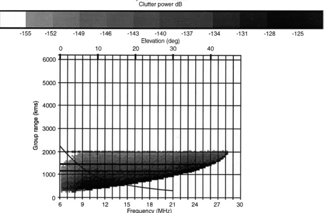
In order to examine the effect of sporadic-E layers, a single, horizontally stratified Es layer of unlimited extent has been used. For convenience a quasi-parabolic layer has been assumed and the analytical ray-tracing program, QPSHEL (an analytical ray-tracing program using mul-tiple quasi-parabolic layers, Dyson and Bennett, 1989), used to calculate the corresponding backscatter ionogram trace. Figure 3 shows the result for a layer 1 km thick, centred at a height of 100 km and with a critical frequency of 5 MHz. The ionogram was calculated utilising Jindalee

Fig. 2a–d. Examples of Jindalee backscatter ionograms with spo-radic-E echoes from specific events discussed in detail. Times are in UT

antenna information. Also shown in Fig. 3 is a curve representing the elevation angle as a function of group path.

If the Es layer is limited in horizontal extent so that it subtends a limited range of elevation angles at the trans-mitter, the backscatter ionogram trace will consist of only a segment of the ionogram trace synthesised for the un-limited layer. This is illustrated in Fig. 3 for an Es layer reflecting rays launched at elevation angles between 5° and 8°. The echo trace is now just a narrow segment which will be superimposed on the echo traces of the background ionosphere giving an ionogram similar to examples shown in Figs. 1 and 2.

The exact shape, thickness and frequency range of the Es trace will depend on the height and critical frequency of the layer, and on the spatial extent and location which

determines the range of elevation angles of rays reflected by the layer. The actual thickness of the layer (assuming it lies in the range 0.5—5 km) has little effect on the Es traces. If the layer height and critical frequency are uniform within the Es cloud and they can be measured by a vertical or an oblique sounder, then the size and position of the Es cloud in the direction of the ray path can be determined by simple geometrical calculations from the observed range of group paths of the Es trace.

2.2 The behaviour of Es clouds

The spatial extent of sporadic-E clouds can be estimated from the eight backscatter ionograms obtained simulta-neously for propagation at different azimuth angles. Two examples are presented from the observations obtained on days 84 and 102. Figure 4 shows an example of a sporadic-E cloud located using the method outlined in Sect. 2.1. The sporadic-E layer height was determined

Fig. 3. Backscatter ionogram signature for a single blanketing spo-radic-E layer. The curved line shows the variation of elevation angle with group range (scale at top of Fig.). The dark horizontal lines show

boundaries of the echoes for a sporadic-E patch illuminated by rays transmitted between 5° and 7° elevation

Fig. 4. Sporadic-E cloud above northern Australia on day 84, 1990 at 1330 UT. The radial lines out of Alice Springs indicate the direc-tions of each of the 8 radar beams

using oblique ionograms obtained over the Alice Springs—Darwin path. While this height may not neces-sarily be exactly the same for other azimuths, the assump-tion of a constant height does not introduce large errors. The azimuth angles of the different beams of the backscat-ter sounder are also shown in Fig. 4.

In this example, the Es cloud was observed on six of the eight azimuthal beams of the backscatter sounder. The

extent of the cloud was between 500—800 km in range and 30°—80° in azimuth. Figure 2a shows the backscatter iono-gram observed with beam 3 at this time.

Another example is shown in Fig. 5 for day 102, 1990 at 1445 UT. This time several patches of sporadic-E were observed at different azimuth angles and at different dis-tances from the backscatter radar. The two distinct Es traces observed on beam 4 near this time are shown in Fig. 2b. (While there is some suggestion of structure in the more distant trace, this was not evident on adjacent beams.)

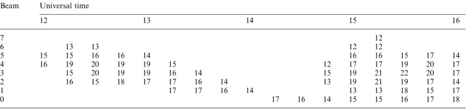
The evolution, and dynamics of Es clouds can be studied from backscatter data obtained by the different radar beams over a period of time. Velocities can be determined by plotting the locations of the sporadic E clouds, as illustrated in Figs. 3 and 4, and calculating the distance traversed by clouds over a period of time. The accuracy of the velocities obtained in this way is about 10%. The evolution of a cloud can conveniently be dis-played as a table showing the maximum frequency, fmEs, reflected from the cloud for each beam as a function of time. An example is shown in Table 1 where it is evident that two clouds were observed. Each one extended about 30—80° in azimuth and lasted about 2 h. These fmEs results were obtained at approximately 15 min intervals during the period 1200—1630 UT on day 115, 1990. It is apparent from the table that two large distinct sporadic-E clouds formed during this period. The first moved off southwest-ward with a velocity of 80 m s~1 to be followed by a

Table 1. Table showing the maximum frequency (fmEs) reflected from sporadic-E clouds for each beam, as a function of universal time, day 115, 1990. (Times refer to the beginning of a 15-min period, i.e. 13 refers to the period 1300—1314 UT)

Beam Universal time

12 13 14 15 16 7 12 6 13 13 12 12 5 15 15 16 16 14 16 16 15 17 14 4 16 19 20 19 19 15 12 17 17 19 20 17 3 15 20 19 19 16 14 15 19 21 22 20 17 2 16 15 18 17 17 16 14 13 19 21 19 17 14 1 17 17 16 14 13 13 18 15 17 0 17 16 14 15 15 16 17 18

Fig. 5. Sporadic-E cloud above northern Australia for day 102, 1990 at 1437 UT

second which remained essentially stationary throughout its growth and delay.

Figure 2c shows the backscatter ionogram observed at 1324 UT on beam 4. At the next observation time, an Es trace very similar in form to that of Fig. 3 was observed on beam 3 (Fig. 2d). At this time there was no discernable corresponding Es trace on beam 4. There is apparent movement of this Es cloud. Notice that the determination of fmEs depends upon the threshold level chosen. It is also complicated by signal contributions due to antenna side lobes.

3 Discussion

The formation and movements of Es clouds were studied for 5 days during the period March—April, 1990. While the aim of this preliminary study was to develop techniques for the study of sporadic-E using the Jindalee radar sys-tem, some general comments on sporadic-E can be made from the observations.

Usually, 2—3 clouds were observed each day, mainly during the evening and up to midnight. The observed clouds extended between 30—80° in azimuth and 150—800 km in range. Whilst there is a lack of other

comparable measurements with which to compare our results in detail, we note that these cloud sizes are in agreement with fixed frequency backscatter results ob-tained in the northern hemisphere (Tanaka, 1979). The life times of the clouds detected in this study were between 1—4 h. Tanaka (1979) observed similar lifetimes during winter but in summer observed clouds to last for up to 10 h. Harwood (1961) observed average lifetimes of 2 h.

The clouds observed in this study were either station-ary or drifted generally westward with velocities of up to 80 m s~1. On one occasion we observed an eastward vel-ocity of about 150 m s~1 which was inconsistent with the other results. The average drift velocities observed by other workers were around 50 m s~1 and the drift direc-tion was usually west to southwest (Tanaka, 1979; Kolawole et al., 1978; Harwood, 1961).

4 Conclusions

The backscatter sounder ionograms obtained as part of the Jindalee Frequency Management System contain a wealth of information on ionospheric structure and behaviour in the northwest Australian region. While these ionograms can be very complicated and difficult to inter-pret, this initial study has shown that they can readily be used to study the behaviour of sporadic-E layers, parti-cularly their spatial extent, motion and evolution with time. Though analytical ray tracing has limitations, we have shown that it can produce the narrow traces asso-ciated with Es patches and thus enable us to determine the location and extent of sporadic-E clouds.

In this initial study of 5 days in March—April 1990, 2—3 clouds were observed each day, mainly during the evening and up to midnight. The clouds lasted from 1—4 h and extended between 30—80° in azimuth and 150—800 km in range. The clouds were mostly stationary or drifted west-ward with velocities of up to 80 m s~1.

Acknowledgments. We would like to thank Drs. B. D. Ward and F.

G. Earl, from H.F.R.D., for supplying Jindalee backscatter iono-grams. CJR wishes to thank D.S.T.O. for their financial support and ZH thanks La Trobe University for the award of a Distinguished Visiting Fellowship.

Topical Editor D. Alcayde´ thanks P. Prikryl for his help in evaluating this paper.

References

Dyson, P. L., and J. A. Bennett, Ionospheric ray tracing calculations: applications to backscatter ionogram synthesis, Final Contract Report Part 2, Surveillance Research Group, DSTO, Salisbury, 12 February 1989.

Earl, G. F., and B. D. Ward, The frequency management system of the Jindalee over-the-horizon backscatter HF radar, Radio Sci., 22, 275, 1987.

Harwood, J., Some observations of the occurrence and movements of sporadic E ionization, J. Atmos. ¹err. Phys., 20, 243, 1961. Kolawole, L. B., and H. Derblom, Skywave backscatter studies of

temperate latitude Es, J. Atmos. ¹err. Phys., 40, 785, 1978. Tanaka, T., Skywave backscatter observations of sporadic-E over

Japan, J. Atmos. ¹err. Phys., 41, 203, 1979.

Whitehead, J. D., Recent work on mid-latitude and equatorial sporadic-E, J. Atmos. ¹err. Phys., 51, 401, 1989.

.