HAL Id: hal-00316264
https://hal.archives-ouvertes.fr/hal-00316264
Submitted on 1 Jan 1996
HAL is a multi-disciplinary open access
archive for the deposit and dissemination of sci-entific research documents, whether they are pub-lished or not. The documents may come from teaching and research institutions in France or abroad, or from public or private research centers.
L’archive ouverte pluridisciplinaire HAL, est destinée au dépôt et à la diffusion de documents scientifiques de niveau recherche, publiés ou non, émanant des établissements d’enseignement et de recherche français ou étrangers, des laboratoires publics ou privés.
A comparison of EISCAT and Dynasonde measurements
of the auroral ionosphere
K. J. F. Sedgemore, P. J. S. Williams, G. O. L. Jones, J. W. Wright
To cite this version:
K. J. F. Sedgemore, P. J. S. Williams, G. O. L. Jones, J. W. Wright. A comparison of EISCAT and Dynasonde measurements of the auroral ionosphere. Annales Geophysicae, European Geosciences Union, 1996, 14 (12), pp.1403-1412. �hal-00316264�
Ann. Geophysicae 14, 1403—1412 (1996) ( EGS — Springer-Verlag 1996
A comparison of EISCAT and Dynasonde measurements
of the auroral ionosphere
K. J. F. Sedgemore1, P. J. S. Williams1, G. O. L. Jones2, J. W. Wright1
1 Adran Ffiseg, Prifysgol Cymru Aberystwyth, Ceredigion SY23 3BZ, Wales 2 British Antarctic Survey, NERC, Cambridge CB3 0ET, England
Received: 26 February 1996/Revised: 13 May 1996/Accepted: 15 May 1996
Abstract. Incoherent-scatter radar and ionospheric sounding are powerful and complementary techniques in the study of the Earth’s ionosphere. The work presented here involves the use of the Tromsø Dynasonde as a cor-relative diagnostic with the EISCAT incoherent-scatter radar. A comparison of electron-density profiles shows how a Dynasonde can be used to calibrate an incoherent-scatter radar and to monitor changes in the system. Sky-maps of the direction of Dynasonde echoes are compared with EISCAT-derived density profiles to illustrate how a Dynasonde can be used to measure the drift velocity of auroral features. Vector velocities fitted to Dynasonde echoes are compared with EISCAT-derived plasma vel-ocities. The results show good agreement when the data are taken during quiet to moderately active conditions and averaged over time scales of 30 min or more.
1 Introduction
The auroral ionosphere has such complex spatial struc-ture and changes so rapidly that no single method of observation will give a complete picture. Progress will depend on co-ordinating results from a number of differ-ent instrumdiffer-ents. The aim of the presdiffer-ent work is to compare simultaneous measurements made by an inco-herent-scatter radar (EISCAT) and a digital ionosonde (Dynasonde), to produce valuable scientific results in their own right and to help validate Dynasonde measurements made by the British Antarctic Survey at Halley. Previous comparisons of electron-density profiles (Wright et al., 1988, 1990) have shown reasonable agreement during quiet conditions, but during more active conditions the Dynasonde indicated E-region structure where the elec-tron density was a factor of over two greater than the average value measured by EISCAT. This small-scale
Correspondence to: K. J. F. Sedgemore
structure requires further study, as it alters our picture of auroral activity. The input flux of energetic particles is assumed to be proportional to N2e, where Ne is the elec-tron density, and asSN2eT'SNeT2, the true energy input due to particle precipitation during magnetospheric sub-storms may be considerably larger than indicated by aver-age values.
Ionosondes are relatively cheap when compared with other ionospheric radar systems and are therefore used extensively, monitoring both long-term temporal and large-scale spatial variations in the ionosphere (Villard, 1976). Conventional, analogue ionosondes have made an invaluable contribution to radio science, but they have several limitations, based on the fact that not all the information in the returned signal is used. Much more information than the simple time of flight of a reflected HF radar pulse can be derived if the echo phase is mea-sured. With phase information and a spaced receiv-ing-antenna array, it is possible to determine the arrival direction, polarisation and Doppler shift of the echoes.
The Tromsø Dynasonde is one of six digital sounders designed and constructed at the Space Environment La-boratory in Boulder, USA, between 1975 and 1979 (Wright and Pitteway, 1979a, b; Grubb, 1979). Two iden-tical receivers are tuned to whichever frequency is being transmitted, and six dipole receiving antennas are de-ployed in an array. Under normal geophysical conditions, echoes with a signal-to-noise ratio of 20 dB or more are recorded at frequencies above 1 MHz. The echo polarisa-tion is determined by comparing the phases recorded on pairs of orthogonal dipole antennas, and the horizontal distance of echoes from the zenith by recording the phases on spatially separated antennas. The variation of phase with frequency is determined by transmitting some pulses with a slight frequency increment, leading to an improved measurement of the virtual range by the principle of stationary phase (Whitehead and Kantarizis, 1967; Paul
et al., 1974).
The time dependence of echo phase is measured within the short span (0.03 s) of a pulse set, whilst the alternative ‘B-mode’ permits a similar estimate over longer spans
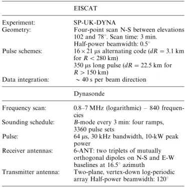
Table 1. EISCAT and Dynasonde configurations for the Special Programme, SP-UK-DYNA
EISCAT
Experiment: SP-UK-DYNA
Geometry: Four-point scan N-S between elevations 102 and 78°. Scan time: 3 min.
Half-power beamwidth: 0.5°
Pulse schemes: 16]21 ls alternating code (dR"3.1 km for R(280 km)
350ls long pulse (dR"22.5 km for R'150 km)
Data integration: &40 s per beam direction Dynasonde
Frequency scan: 0.8—7 MHz (logarithmic) — 840 frequen-cies
Sounding schedule: B-mode every 3 min: four ramps, 3360 pulse sets
Pulse: 64ls, 30 kHz bandwidth, 10-kW peak power
Receiver antennas: 6-ANT: two triplets of mutually orthogonal dipoles on N-S and E-W baselines at 16.5° azimuth
Transmitter antenna: Two-plane, vertex-down log-periodic array Half-power beamwidth: 120°
(Wright and Pitteway, 1979a). The equivalent ‘Doppler shift’ can be expressed as a line-of-sight velocity. By com-bining these velocities and the direction cosines for a col-lection of echoes, a vector velocity may be obtained by least-squares estimation (Wright and Pitteway, 1994; Jar-vis, 1995).
2 Electron-density profiles
By comparing electron-density measurements, it is pos-sible to use an ionosonde to calibrate an incoherent-scat-ter radar (ISR). In the process, it is shown how true-height profile inversion of ionosonde data may be improved.
With ISR systems, received power is used to derive relative electron densities, and analysis of ISR data in-volves the use of a calibration factor to derive absolute values of electron density. This calibration factor is often referred to as the system constant, but in practice it can change with time, as there are several different parameters contributing to it. The relative electron density at a given range R can be derived to a good approximation from the power of the echo, given by:
Ps"0.016cpe[¸T¸RPpAq]R2(1#¹e/¹i)Ne ,
where c is the speed of light in vacuo, andpe the electron scattering cross-section (Rishbeth and Williams, 1985). The terms within square brackets are system factors rep-resenting the loss factor in the feed system during trans-mission and reception, the peak power transmitted, the effective collecting area of the antenna, and the pulse length, respectively. ¹e and ¹i are the electron and ion temperatures, respectively. The measurement of Ps by comparison with an injection of noise power, together with the expression 0.016cpe[¸T¸RPpAq] constitute the calibration factor which must be used to derive an abso-lute value of electron density. In practice, several of the parameters involved, such as losses in the feed, antenna gain and the exact value of noise-injection power, may change with time. As a result, ISR measurements give reliable and accurate relative values of electron density both below and above the F-region peak. It is not usually possible, with an ISR alone, to obtain an absolute calib-ration to match the accuracy of the relative measure-ments.
With ionosondes, electron densities are derived from plasma frequency measurements and these can be cali-brated with very high accuracy. An ionosonde measures group range as a function of frequency from the time-of-flight of a pulse, but to allow for group retardation this function must be inverted to convert virtual height into true height. There are a number of methods for deriving true-height profiles, the most widely used of which is the Titheridge Overlapping Polynomial Analysis, known commonly asPOLAN(Titheridge, 1967, 1985). Real-height
inversion cannot provide direct information from ‘valley minima’ in the profile, nor from heights above the F2 peak.
The combination of an ISR and an ionosonde can provide full and accurate profiles of absolute electron density. The simplest procedure is to compare F-region peak densities alone, and this is sufficient to determine the ISR calibration factor. A more rigorous analysis involves a comparison of full electron-density profiles. For example, problems are often encountered with POLAN
-fitted valley minima (Titheridge, 1990). The width and depth assumed for the valley can have a significant effect on the height of the fitted F2 peak. This problem has been encountered also by Chen et al. (1994) in their comparison of electron-density profiles from the Kangerlussuaq (form. Søndre Strømfjord) ISR and a co-located Digisonde.
The data in the following comparison are from a UK Special Programme, SP-UK-DYNA. In this experiment, the EISCAT UHF radar performs a four-point north-south scan every 3 min, and the data are compared with Dynasonde soundings taken every 3 min. This is done primarily in order to provide a longer time-lag over which to measure phase changes due to Doppler shifts. Table 1 outlines the experimental configurations for EISCAT and the Dynasonde.
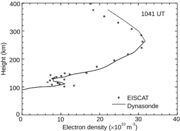
The electron-density profiles shown in Fig. 1 come from the morning of 20 May 1994, during very quiet conditions. The relevant ionogram shows very little spread F, indicating that the ionosphere was plane-strat-ified to a good approximation and thus ideal for profile comparison and calibration-factor evaluation.
The EISCAT profile below 150 km is derived using an alternating-code pulse modulation, and above 150 km altitude using long pulses. Note the large scatter in the
E-region points, due to a transmitter problem that limited
the power available during this experiment so that the signal-to-noise ratio was lower than usual. Despite the scatter, it is possible to see the outline of the E region, with
0 0 10 20 30 40 EISCAT Dynasonde Electron density ( 10 m )× 10 -3 1041 UT 100 200 300 400 Heigh t (km)
Fig. 1. Combined electron-density profiles from EISCAT and the Dynasonde, taken at 1041 UT, 20 May 1994, during the experiment SP-UK-DYNA. The EISCAT data are of the alternating-code type below 150 km and the long-pulse type above 150 km. They are based on a revised calibration factor derived from Dynasonde-measured F-region peak densities. The Dynasonde profile has been generated usingPOLAN
its peak at around 110 km altitude. The long-pulse data, with pulse length 350ls and gate separation 22.5 km, have higher signal-to-noise ratio and provide reliable re-sults up to a height of 350 km, well above the F2 peak. There is one problem with the long-pulse data: if the F2 peak is sharp, convolution with a relatively long pulse leads to a systematic underestimate of electron density (Kirkwood et al., 1986; Wright et al., 1988). This is less of a problem when the peak is well rounded, and in the present case the underestimate is around 2%. It is possible to correct EISCAT-derived profiles for this effect using Fourier methods, but in this case it is the ratio of densities that is of primary interest. Instead, the Dynasonde-de-rived densities have been adjusted downwards using the same smoothing function as applied to the EISCAT data (Turunen, 1986).
The shape of the EISCAT-derived E-region valley has been used to force the shape of thePOLANvalley.
Al-though the peak density is unaffected by the inversion, any error in the boundary conditions will propagate up the profile affecting both its general shape and the height of the F-region peak. With no reference curve such as that provided by EISCAT, it is difficult to fit accurate electron density profiles to high-latitude ionosonde data. This problem has been encountered by Heaton et al. (1995) in their attempt to verify density profiles generated by the technique of ionospheric tomography. Although a Dyna-sonde is incapable of receiving echoes from above the F2 peak, thePOLANcurve is extrapolated upwards from this
point by over 100 km (1.5 scale heights) using a Chapman function. This model may not always apply at high latit-udes, and it can be seen in this typical case that above the peak the agreement is not so good.
The EISCAT data shown in Fig. 1 were analysed ini-tially with a calibration factor in use since the beginning of 1993. When the EISCAT results were compared with the POLAN-derived profile, a discrepancy was found,
with EISCAT underestimating the true F2-peak density by 8%. This points to a change in one or more of the EISCAT system factors listed above. Early in 1994, there was a problem with the secondary reflector on the UHF antenna, and this could be the principle cause of the change in the calibration factor. Figure 1 shows the two electron-density profiles with the EISCAT values in-creased by 8% to correct for the apparent change in the calibration factor. With this scaling, very good agreement is obtained for all heights in the F region below the peak. Wright et al. (1988) reported a similar discrepancy in the calibration factor (15%), and various other workers have reported differences of this order. Such uncertainties in EISCAT electron-density measurements are unnecessary and make it difficult to use the radar to verify numerical models. By comparing profiles taken over significant peri-ods of time, it is possible to monitor independently the state of the EISCAT system.
3 Horizontal structure
The EISCAT system can only make measurements along a single, 0.5° radar beam at any one time, and so rapid beam scanning is necessary to establish the existence of horizontal structure in the ionosphere. This procedure is only valid, however, if the ionosphere does not change significantly over the scan period.
Dynasondes, on the other hand, receive echoes from a wide zenith cone, and the arrival directions of the re-ceived echoes can be determined from phase measure-ments using spaced receiving antennas. Under suitable conditions this allows a Dynasonde to monitor the iono-sphere over a wide horizontal area. As a result, an ISR and a co-located Dynasonde make a powerful combination, especially when horizontal variations in electron density, such as that associated with an auroral arc, are moving over the instruments.
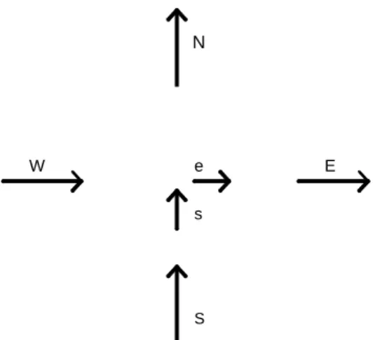
The geometry of echo-location determination is illus-trated in Fig. 2. The apparent distance from the zenith in the horizontal plane at the echo altitude is given by
D"xR@/d, where x is the path difference between the
signals received by a pair of antennas, R@ the time-of-flight (group) range and d the antenna spacing. In terms of phase, x can be expressed as/j/2n, where /"/1!/2 is the difference in phase between the two antennas, and j the radar wavelength. Assuming that the wave front is phase coherent over the scale of the antenna array, the zenith distance is given by:
D"/j
2n·
R@ d .
When the antenna spacing is greater than half the wavelength, the value of / has an ambiguity of $2nN, where N"0, 1, 2, . . . , . This results in aliasing of the derived skymap position to a grid of many possible points in the ionosphere, with the number of possible echo loca-tions inversely proportional to the wavelength. Choosing an appropriate antenna baseline involves a trade-off
N E S W s e
Fig. 3. Dynasonde receiving-antenna configuration used for the experiment SP-UK-DYNA. The six dipoles are arranged along the diagonals of a 100 m square, giving a N-S, W-E spacing of 141 m, and are spaced along the diagonals in the ratios 0 : 2 : 3 from the north and west (Pitteway and Wright, 1992)
Fig. 2. Vertical section through diagonally opposite Dynasonde receiving antennas, for an echo received from a distance D from the zenith (after Dudeney and Jarvis, 1986)
between precision and aliasing. Directional resolution is inversely proportional to antenna spacing, but so is the angle at which aliasing occurs (Dudeney and Jarvis, 1986). The antenna configuration most often used at Tromsø consists of six dipoles arranged along the diagonals of a 100-m square, as illustrated in Fig. 3 (Pitteway and Wright, 1992).
At high latitudes, tilts and localised maxima in electron density, caused by ionospheric features such as the pole-ward edge of the mid-latitude trough, F-region enhance-ment associated with the cusp, intense sporadic-E layers, auroral arcs and blobs, can result in skymaps with echoes received well away from the zenith. With the Dynasondes operated at Tromsø and Halley, echoing regions have been tracked at apparent distances as large as 900 km from the zenith: hence the importance of developing
methods for minimising aliasing and evaluating the true skymap position.
Of special interest in joint observations with EISCAT are those cases where a localised maximum in electron density drifts steadily over the instruments. The iso-ionic contours associated with such a feature are often close to ellipsoidal, and the feature will give echoes over a wide range of zenith angles. By studying Dynasonde skymaps, it is possible to track the movement of such features in consecutive soundings (Lanchester et al., 1993).
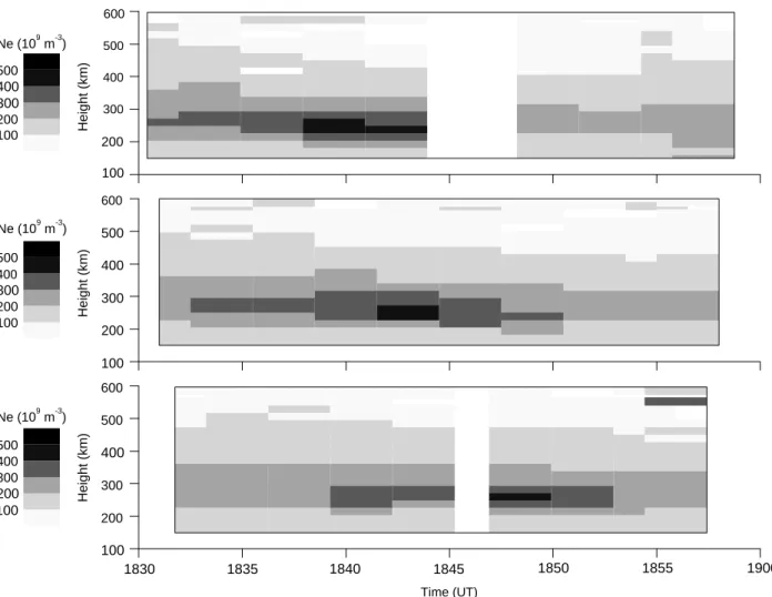
During the SP-UK-DYNA experiment of 23 May 1994, between 1830 and 1900 UT, a region of enhanced electron density at around 240 km altitude with a peak value of around 4]1011 m~3 was seen moving in a north-south direction through the EISCAT field-of-view. The electron density contours are shown in Fig. 4. This F-region density enhancement was seen by EISCAT in three beam eleva-tions: 96° (north), 90° and 84° (south) along a north-south meridian, appearing first at 1836 UT, in beam elevation 96°, and disappearing from view at 1850 UT in beam elevation 84°. Tristatic EISCAT measurements at 278 km altitude show the magnetic north-south plasma velocity as being 125$25 m s~1 at this time. This is consistent with the estimated drift velocity for the feature of 140$30 m s~1, determined by analysing the motion of the enhancement shown in Fig. 4. It is thus reasonable to assume that the feature is moving with the general plasma flow, especially as the measured plasma velocity is approx-imately constant with time and position during this period. Figure 5 shows a time series of three Dynasonde maps, each separated by 3 min intervals. In these sky-maps, northward echolocation is plotted against virtual height. In addition to the usual strong echoes coming from the field-aligned direction, from 1843 through to 1849 UT there was a patch of echoes seen drifting south-ward, appearing first around 40 km north at 1843 UT, then slightly to the south at 1846 UT. The peak electron densities, derived from reflection frequencies, are consis-tent with the corrected EISCAT measurements. SP-UK-DYNA does not monitor any east-west movement of the feature, but Dynasonde skymaps of eastward echoloca-tion show no significant zonal drift. The same F-region density enhancement is undoubtedly seen by both instru-ments, with the same peak densities and moving in the same way. It should be noted that this comparison has been made possible only through the relatively rapid scan of the EISCAT radar during the SP-UK-DYNA experi-ment.
A continuous record of the horizontal movement of a region of enhanced electron density, such as an auroral feature, is of direct value in giving its drift velocity and physical dimensions. Whilst the study of small-scale struc-ture is of scientific interest in its own right, there is a fur-ther justification for employing an ISR and a Dynasonde together. When a second antenna is added to the EISCAT Svalbard Radar (ESR) for split-beam operation, the drift velocity of an auroral feature, which a Dynasonde at Longyearbyen would be able to measure, will indicate the appropriate time-lag for combining the two components of plasma velocity measured by the ESR to give a single, unbiased vector (Williams, 1995).
Time (UT) 100 200 300 400 500 600 Height (km) 100 200 300 400 500 100 200 300 400 500 600 Height (km) 100 200 300 400 500 100 200 300 400 500 600 Height (km) 100 200 300 400 500 Ne (10 m )9 -3 1830 1835 1840 1845 1850 1855 1900 Ne (10 m )9 -3 Ne (10 m )9 -3
Fig. 4. Time series of EISCAT long-pulse electron-density contours taken from the experiment SP-UK-DYNA, 23 May 1994. The panels, from top to bottom, correspond to beam elevations 96°
(north), 90° and 84° (south). An F-region feature is seen first in the top panel at 1838 UT. It then moves southwards through the other two positions, finally disappearing at around 1850 UT
4 Vector velocities
A third important comparison applies to the conditions under which a Dynasonde can make reliable measure-ments of sustained plasma convection velocity. The results of the comparison can be used to optimise future joint work and to validate drift measurements made where a Dynasonde operates on its own, as at Halley, or at Tromsø and Longyearbyen, when no operating time is available for the incoherent-scatter radars.
The EISCAT radar makes measurements of the Dop-pler frequency shift of echo returns, and from these, plasma vector velocities can be derived either tristatically or monostatically (i.e. beam swinging) (Williams et al., 1984; Jones et al., 1986). The Dynasonde can also estimate a vector velocity by making simultaneous measurements of echo Doppler shift in different directions and at differ-ent heights. Under some circumstances, these Doppler measurements may be interpreted as physical movements of ionospheric plasma (From et al., 1988). This is because echo Doppler shifts are affected by both the plasma motion and by variations in the refractive index along the ray path. The principle of the method is to combine the
Doppler shifts and direction cosines of a number of echoes, and so form an estimate of the velocity vector for the selected volume. The Doppler velocities are given by:
»*"j 4n
d/
dt"X · »X#½·»Y#Z · »ZR@
whered/ is the phase change from the transmitted refer-ence phase, X, ½, Z the echo-location components, and »X, »Y, »Z the components of the velocity vector (Wright and Pitteway, 1994). The sampling volume is specified by a virtual height and frequency range, and an optional angular filter. A velocity vector can then be fitted to the selected echoes using either least squares (e.g. the VFIT
programme described in Wright and Pitteway, 1994) or singular value decomposition (Jarvis, 1995). A theoretical advantage of the latter is that it avoids unrealistically large solutions that can occur if the equation matrix is ill-conditioned. In practice, least-squares fitting produces results entirely consistent with those from singular value decomposition, andVFITwas used in the present analysis.
The philosophy behind this approach is qualitatively different from that of EISCAT tristatic velocities, where
1846 Vir tual height (km) 400 300 200 100 1849 Northward echolocation (km) c -200 -100 0 100 200 1843 a b Vir tual height (km) 400 300 200 100 Vir tual height (km) 400 300 200 100
the sampling volume is relatively small. The method out-lined requires that the spatial distribution of echoes be as large as possible in order to minimise the geometrical estimation error. Hence, a compromise must be made: choose a large sampling volume and derive a reliable estimate of the average velocity vector within that volume, or achieve better spatial resolution by restricting the sampling volume at the cost of increased error.
It is possible to compare the Dynasonde method with ISR beam swinging, in that with monostatic measure-ments, velocity samples from a large volume are combined to give a single vector. This technique was used by Scali
et al. (1995) in their comparison of ISR and Digisonde
velocities at Kangerlussuaq. The results from both instru-ments are subject to error if there are temporal and/or spatial variations in plasma velocity on scales comparable with, or smaller than the sampling volume and integration time. It should be remembered that normal ISR beam swinging does not give an average velocity over the scan time and area covered, as any variations in the velocity over the whole scan generate spurious velocities by the process known as mixing (Etemadi et al., 1989). The differ-ence is that in the case of a Dynasonde, the measurements are made (virtually) simultaneously as the entire sounding is completed in far less time than the usual scanning cycle for an ISR. Any strong spatial gradients in plasma velocity over the volume sampled may still introduce the risk of spurious velocity calculations.
As with Dynasonde echo-location determination, alias-ing is also a problem in Doppler velocity estimation. The line-of-sight velocity is estimated by taking the phase change of an echo over the time interval between one or more pulses at the same frequency. Aliasing is unlikely to occur at lower radio frequencies but it is very sensitive to the time interval used. The phase will alias at $90° in a four-pulse set, where the pulses are separated by 0.01 s, giving an aliasing interval of 150 m s~1 for a typical F-region reflection frequency of 4 MHz. If the Doppler vel-ocity is increasing with time or frequency, a value of 150 m s~1 can flip to about !150 m s~1. Whilst aliasing can be a serious problem, its effects can be countered through careful inspection of the data (Pitteway and Wright, 1992).
The data in the following comparison are from the Common Programme CP-1-K of 8 and 9 June 1994. CP-1 is a fixed-position UHF experiment, where the beam is aligned along the direction of the local magnetic field. Data dumps occur every 5 s, though in this case the raw data were post-integrated over a 2 min period. EISCAT
F-region vector velocities at 278 km were derived using
the tristatic method, the only possible method with a fixed radar beam.
b
Fig. 5a–c. Time series of Dynasonde skymaps showing the north-south drift of an F-region electron density enhancement (arrowed) from 1843 to 1849 UT during the experiment SP-UK-DYNA, 23 May 1994. The feature is at a real height of around 240 km. The local magnetic field line is shown on these plots, the dip angle at Tromsø being 77.5°
0 EISCAT Dynasonde 0200 2100 1600 0700 Time (UT) 1200 1700 2200 -800 -400 400 800 Vper pE (m s ) -1
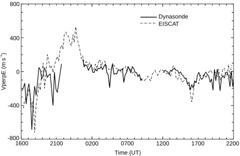
Fig. 6. Time series of EISCAT and Dynasonde F-region velocities from the experiment CP-1-K, 8—9 June 1994. The eastward component of plasma velocity perpendicular to the geomagnetic field line is shown. Both curves are 12 min running averages
The Dynasonde B-mode soundings were separated by 3-min intervals. All echoes with reflection frequencies in the range 2.8—8 MHz, with (virtual) ranges between 300 and 500 km, and within a 20° zenith cone, were included in the analysis. The frequency range is typical for the whole F region, whilst the range spread selects a sampling volume based on the F2 peak — i.e. centred on the intersection height of the EISCAT beams. The velocity vectors were fitted using a least-squares approach, though the experimental arrangement differed in several respects from that given in Table 1. In this experiment, a four-antenna subset of this configuration was used in order to minimise the interference caused by other nearby HF radio equipment.
The eastward component of plasma velocity perpen-dicular to the field line is shown in Fig. 6, from 1600 UT on 8 June to 2200 UT on 9 June. Both EISCAT and Dynasonde values are 12 min running averages. This has been done in order to reduce the scatter in points and select the large-scale features in the velocities. Looking first at the EISCAT curve, which is assumed to be a cor-rect representation of the time variation of velocity in a single fixed volume of the F region, a clear west-to-east transition in plasma flow (the Harang discontinuity) can be seen, centred at around 1900 UT on 8 June, and on the following day a small westward flow peaking at magni-tude 350 m s~1, starting at 1400 UT and lasting for about 4 h. Apart from these relatively small velocity excursions, the rest of the 30 h period is rather quiet, with little eastward plasma movement recorded over 100 m s~1. The errors in the EISCAT velocities, when averaged over 12 min, are rather large (typically 60 m s~1), as is common for tristatic measurement with low signal-to-noise ratio. Despite this, it is still possible to resolve the features with the error bars included.
The Dynasonde-derived eastward component of vel-ocity is superimposed on the EISCAT velocities in Fig. 6. Apart from two gaps in the data, caused by F-region blackout, it can be seen that the two curves are in modest
agreement. HF radio blackout is caused either by strong absorption or by an enhanced E layer when strong reflec-tions from the E region obscure those from higher up. Unfortunately for studies of the auroral ionosphere with HF radar, blackout occurs commonly during the most geophysically interesting events, such as auroral precipita-tion and substorms. Such ‘blanketing’ is fairly extensive, with only a few echoes passing through small ‘holes’ in the
E region.
Looking in detail at the comparison, it can be seen that the transition from a velocity of !700 m s~1 (westwards) to #500 m s~1 (eastwards) is followed by the Dynasonde up to the Harang discontinuity, after which the F region blacks out until just after 2400 UT. From around 1900 to 2200 UT on 8 June, skymaps show the presence of some small-scale F-region electron-density patches, concen-trated in a very small region around the zenith and biased slightly towards the north, away from the EISCAT beam. This bias is a likely cause of the sometimes substantial disagreement with EISCAT during this period, since the two instruments are sampling different volumes of the convection flow. The period of blackout is marked by a strong precipitation event where the E-region peak electron density is over 4]1011 m~3. After 2400 UT, the
F-region echoes return, as does reasonable agreement,
during a quiet period that lasts until around 0900 UT. There then follows a 3 h period of blackout, due this time to total absorption of the HF radio waves. Reasonable agreement returns with the end of the period of HF absorption. It is at this point that EISCAT shows the plasma undergoing a small westward surge in velocity to a maximum of around 400 m s~1. The Dynasonde follows this excursion, though underestimating the magnitude of the velocity at its peak. After 1700 UT, the quiet iono-sphere returns.
The agreement between the EISCAT and Dynasonde velocities is best quantified by calculating the correlation coefficient for the two sets of data. To do this, both sets of data are averaged over intervals of 6, 12, 18 min, and so on
Table 2. Correlation between EISCAT and Dynasonde measure-ments of plasma velocity during the experiment CP-1-K, 8—9 June 1994
Integration Correlation coefficient Correlation coefficient time (min) for east-west for north-south
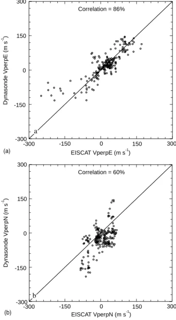
velocities (%) velocities (%) 6 52 25 12 63 36 18 68 43 24 70 48 30 75 49 36 75 55 42 75 57 48 78 58 54 86 60 60 82 63 Correlation = 86% Correlation = 60% a EISCAT VperpE (m s )-1 EISCAT VperpN (m s )-1 Dynasonde Vper pE (m s ) -1 Dynasonde Vper pN (m s ) -1 300 150 -150 0 -300 -300 -150 0 150 300 -300 -150 0 150 300 300 150 -150 0 -300 b
Fig. 7a, b. Correlation between EISCAT and Dynasonde velocities during the experiment CP-1-K, 8—9 June 1994. a East-west com-ponent, and b north-south component; all values are 54 min aver-ages
up to 60 min. Table 2 shows the correlation coefficients derived in this way. The strongest correlation is seen in the case of the east-west velocities where the coefficients in-crease steadily as the data is integrated over longer time intervals, reaching a maximum of 86% for an integration time of 54 min. Even with such long time averaging, the major features in both velocity distributions remain clear. The north-south velocities are much smaller and hence affected more by random errors. Here too however, the correlation coefficients show a steady increase with integ-ration time, reaching a maximum of 63% for an integra-tion time of 60 min. Figure 7a shows a scatter plot of the east-west velocity as measured by EISCAT and the Dyn-asonde, averaged over 54 min, and Fig. 7b the corre-sponding north-south velocities.
The main conclusion for these initial comparisons is that there is a high correlation between the changes in plasma velocity on a time scale of 30 min or more as measured by EISCAT and the Dynasonde, but poorer agreement for short term variations. This is to be ex-pected, as the F-region plasma velocity has two compo-nents:
f A general convection driven by the two-cell pattern of electric potential, controlled largely by the interplan-etary magnetic field (IMF) (Heppner and Maynard, 1987). Lockwood (1991) has shown that major changes in the prevailing direction of the IMF occur typically after intervals of between 30 and 60 min.
f Sudden increases and decreases in plasma velocity that occur locally during the expansion phase of substorms. In many cases these have been identified with narrow bands of greatly enhanced plasma velocity, often less than 20 km wide, lying parallel and adjacent to auroral arcs, where the electric field, and hence the plasma velocity, is very low (Opgenoorth et al., 1990; Lewis
et al., 1994; Lanchester et al., 1996)
As the general convection occurs on a large scale and is steady over periods of up to 1 h, both monostatic and tristatic EISCAT observations should give similar results to the Dynasonde when averaged over such time scales. In the presence of auroral activity, where there are very sharp spatial gradients in plasma velocity, it is to be expected that EISCAT and the Dynasonde will give different
results. In future it may be possible to analyse the Doppler velocities measured by the Dynasonde in different direc-tions, within the framework of a comprehensive elec-trodynamic model of an auroral feature, and so get a bet-ter overall picture than is possible with EISCAT alone. For the time being, all we can report is that routine Dynasonde and EISCAT measurements of velocity some-times show disagreements on a short time scale, but the longer-term averages correlate very well.
In Fig. 7a and b, the line plotted for reference has a unit slope but the slope of the ‘best-fitting’ straight line is more problematic. There are substantial random errors in indi-vidual measurements of velocity whether measured by EISCAT or by the Dynasonde, and in addition when
measurements are made during a period of auroral activ-ity, the two velocities derived may correspond to different volumes. There is therefore no single linear regression algorithm that can be used with any degree of confidence. In the case of Fig. 7a, two algorithms (assuming that all the errors are either in y or in x) both give a slope less than 1.0, but it is clear on examination that this result is strongly influenced by a relatively small number of points, all taken during the period 1730—1900 UT on 8 June. Here, the values derived from EISCAT are in the range !150 to !250 m s~1, while the corresponding values from the Dynasonde are in the range !50 to !150 m s~1. Apart from this small number of points, the data are compatible with a slope of 1.0. The north-south velocities (Fig. 7b) are generally smaller than the east-west and so are more strongly affected by the random errors. Once again, the results are strongly influenced by a small number of points taken during the same disturbed interval.
5 Conclusions
The results described in this paper confirm three ways in which an advanced digital ionosonde, such as the Dyna-sonde, can provide valuable extra measurements to those made by an ISR such as EISCAT.
In measuring profiles of electron density, the strengths and weaknesses of the two instruments are exactly com-plementary. The EISCAT UHF radar can provide an accurate true-height profile of relative electron density from below 100 km to over 500 km, covering any valley between the E and F regions and continuing well into the topside. The Dynasonde can only make direct measure-ments of electron density versus virtual height below the
F-region peak, and can only cover the valley convincingly
with the help of the EISCAT profiles. It does, however, provide absolute values of electron density and can there-fore be used to calibrate the EISCAT results. There is no reason why a combination of the two instruments should not achieve an overall accuracy of 2—3% under normal conditions. A similar combination will be especially valu-able on Svalbard, where at the inauguration of the EIS-CAT Svalbard radar there will be no other method of calibration.
The combination can offer another important contri-bution to our understanding of the auroral ionosphere on occasions, such as those reported by Wright et al. (1990), where the Dynasonde indicates structure in the E region with electron densities much higher than the average values measured by EISCAT. No examples were detected in our present observations, but these were carried out under relatively quiet conditions near sunspot minimum. The complementary properties of EISCAT and the Dynasonde are also displayed in the mapping of electron density over a wide vertical plane. EISCAT provides con-tinuous and reliable measurements of electron-density profiles in a single direction, but to distinguish temporal and spatial variations it must scan rapidly through a num-ber of pointing directions. This mode is limited by the
minimum dwell time necessary for accurate measurement, and also by the mechanical restrictions imposed by the antenna design. The Dynasonde can receive echoes from a range of zenith angles, and in this way it provides an instantaneous ‘snapshot’ of horizontal structure in the ionosphere. Thus when a well-defined region of enhanced electron density drifts steadily overhead, the Dynasonde will preferentially receive echoes from the feature and hence monitor its horizontal drift. When this occurs, the combination of EISCAT and the Dynasonde is very powerful, as it allows a clear separation of temporal and spatial variations. On Svalbard this combination will be even more important when attempting to monitor the electrodynamics of a steadily drifting auroral feature with a multiantenna, but monostatic ISR.
In assessing the total potential of a Dynasonde/ISR combination, perhaps the most important question still to be answered is whether the velocity measurements made by a Dynasonde can replace the tristatic velocity measure-ments made by an ISR such as EISCAT. The results in this paper must be regarded as preliminary but a clear pattern is indicated.
There can be no question that under very disturbed conditions, where the actual plasma velocity in the iono-sphere can vary from less than 100 m s~1 to more than 4000 m s~1 within a distance of a few kilometres (Lanches-ter et al., 1996), the two instruments will provide signifi-cantly different results. Unless the two instruments are observing precisely the same volume, the measured veloc-ity will be different even if both instruments make perfect measurements. In the case of a Dynasonde, however, it is essential to combine measurements from different vol-umes of the ionosphere to generate a full velocity vector, and while it requires a wide spread of observations to minimise the geometrical errors in such a calculation, such a wide distribution increases the danger of combining velocity components from regions where the true velocity is very different.
The results reported in this paper confirm that under relatively quiet conditions, when the measurements are averaged over a periods of 30 min or more, both instru-ments give a reliable indication of the large-scale convec-tion patterns which apply at high latitudes.
Acknowledgements. The authors are very grateful to the Director and Staff of EISCAT for the data used in this work, and especially for the help and advice provided for the successful operation of the Dynasonde. EISCAT is an international facility supported by Fin-land, France, Germany, Norway, Sweden and the United Kingdom. The authors are also grateful to the staff of the Ionosphere Group at the Rutherford Appleton laboratory for helpful discussions.
Topical Editor D Alcayde´ thanks C. La Hoz and M. L. Parkinson for their help in evaluating this paper.
References
Chen, C. F., B. W. Reinisch, J. L. Scali, X. Huang, R. R Gamache, M. J. Buonsanto, and B. D. Ward, The accuracy of ionogram-derived N(h) profiles, Adv. Space Res., 14, 1243—1246, 1994. Dudeney, J. R., and M. J. Jarvis, A simple graphical method for
de-aliasing digital ionosonde echo location data, Radio Sci., 21, 101—105, 1986.
Etemadi, A., S. W. H. Cowley, and M. Lockwood, The effect of rapid changes in ionospheric flow on velocity vectors deduced from radar beam-swinging experiments, J. Atmos. ¹err. Phys., 51, 125—138, 1989.
From, W. R., Elaine M. Sadler, and J. D. Whitehead, Measuring ionospheric movements using totally reflected radio waves, J. Atmos. ¹err. Phys., 50, 153—156, 1988.
Grubb, R. N., ¹he NOAA SE¸ HF radar system (ionospheric soun-der), NOAA Technical Memo: ERL SEL-55, 1979.
Heaton, J. A. T., S. E. Pryse, and L. Kersley, Improved background representation, ionosonde input, and independent verification in experimental ionospheric tomography, Ann. Geophysicae, 13, 1297—1303, 1995.
Heppner, J. P., and N. C. Maynard, Empirical high-latitude electric field models, J. Geophys. Res., 92, 4467—4489, 1987.
Jarvis, M. J., First observations of F-region plasma flow at Halley, Antarctica, J. Atmos. ¹err. Phys., 57, 1611—1622, 1995. Jones G. O. L., K. J. Winser, and P. J. S. Williams, Measurements of
plasma velocity at different heights along a magnetic field line, J. Atmos. ¹err. Phys., 48, 887—892, 1986.
Kirkwood, S., P. N. Collis, and W. Schmidt, Calibration of electron densities for the EISCAT UHF radar, J. Atmos. ¹err. Phys., 48, 773—775, 1986.
Lanchester, B. S., T. Nygre{ n, M. J. Jarvis, and R. Edwards, Gravity wave parameters measured with EISCAT and Dynasonde, Ann. Geophysicae, 11, 925—936, 1993.
Lanchester, B. S., K. Kaila, and I. W. McCrea, Relationship between large horizontal electric fields and auroral arc elements, J. Geo-phys. Res., in press, 1996.
Lewis, R. V., P. J. S. Williams, G. O. L. Jones, H. J. Opgenoorth, and M. A. L. Persson, The electrodynamics of a drifting auroral arc, Ann. Geophysicae, 12, 478—480, 1994.
Lockwood, M., Flux-transfer events at the dayside magnetopause — transient reconnection or magnetosheath dynamic pressure pulses?, J. Geophys. Res., 96, 5497—5509, 1991.
Opgenoorth, H. J., I. Ha~ ggstro~m, P. J. S. Williams, and G. O. L. Jones, Regions of strongly enhanced perpendicular electric fields adjacent to auroral arcs, J. Atmos. ¹err. Phys., 52, 449—458, 1990. Paul, A. K., J. W. Wright, and L. S. Fedor, The interpretation of ionospheric radio drift measurements — VI, Angle of arrival and group-path (echolocation) measurements from digitized iono-spheric soundings: the group path vector, J. Atmos. ¹err. Phys., 36, 193—214, 1974.
Pitteway, M. L. V., and J. W. Wright, Toward an optimum receiving array and pulse set for the Dynasonde, Radio Sci., 27, 481—490, 1992.
Rishbeth, H., and P. J. S. Williams, The EISCAT ionospheric radar, the system and its early results, Q. J. R. Astron. Soc., 26, 478—512, 1985.
Scali, J. L., B. W. Reinisch, C. J. Heinselman, and T. W. Bullett, Coordinated digisonde and incoherent scatter radar F-region drift measurements at Sondre Stromfjord, Radio Sci., 30, 1481—1498, 1995.
Titheridge, J. E., The overlapping polynomial analysis of ionograms, Radio Sci., 2, 1169—1175, 1967.
Titheridge, J. E., Ionogram analysis with the generalised program POLAN, ¼orld Data Centre A for Solar-¹errestrial Physics, 1985.
Titheridge, J. E., Aeronomical calculations of valley size in the ionosphere, Adv. Space Res., 10, 821—824, 1990.
Turunen, T., GEN-SYSTEM — a new experimental philosophy for EISCAT radars, J. Atmos. ¹err. Phys., 48, 777—785, 1986.
Villard, O. G., The ionospheric sounder and its place in the history of radio science, Radio Sci., 11, 847—860, 1976.
Whitehead, J. D., and E. Kantarizis, Errors in the measurement of virtual height using a phase ionosonde, J. Atmos. ¹err. Phys., 29, 1483—1488, 1967.
Williams, P. J. S., A multi-antenna capability for the EISCAT Svalbard radar, J. Geomagn. Geoelectr., 47, 685—698, 1995. Williams, P. J. S., G. O. L. Jones, and A. R. Jain, Methods of
measuring plasma velocity with EISCAT, J. Atmos. ¹err. Phys., 46, 521—530, 1984.
Wright, J. W., and M. L. V. Pitteway, Real-time data acquisition and interpretation capabilities of the Dynasonde: 1. Data ac-quisition and real-time display, Radio Sci., 14, 815—825, 1979a.
Wright, J. W., and M. L. V. Pitteway, Real-time data acquisition and interpretation capabilities of the Dynasonde: 2. Determination of magnetoionic mode and echo location using a small spaced receiving array, Radio Sci., 14, 827—835, 1979b.
Wright, J. W., and M. L. V. Pitteway, High-resolution vector vel-ocity determinations from the Dynasonde, J. Atmos. ¹err. Phys., 56, 961—977, 1994.
Wright, J. W., R. I. Kressman, T. S. Virdi, and P. N. Collis, Compari-sons of EISCAT and Dynasonde ionospheric measurements: simple to moderately structured plasma densities, J. Atmos. ¹err. Phys., 50, 405—421, 1988.
Wright, J. W., R. I. Kressman, T. S. Virdi, and P. N. Collis, A com-parison of plasma densities by EISCAT and the Dynasonde from auroral altitudes: evidence of intense structure, J. Atmos. ¹err. Phys., 52, 289—303, 1990.