HAL Id: hal-03010626
https://hal.archives-ouvertes.fr/hal-03010626
Submitted on 17 Nov 2020HAL is a multi-disciplinary open access archive for the deposit and dissemination of sci-entific research documents, whether they are pub-lished or not. The documents may come from teaching and research institutions in France or abroad, or from public or private research centers.
L’archive ouverte pluridisciplinaire HAL, est destinée au dépôt et à la diffusion de documents scientifiques de niveau recherche, publiés ou non, émanant des établissements d’enseignement et de recherche français ou étrangers, des laboratoires publics ou privés.
Dissolution Anisotropy of Pyroxenes: A Surrogate
Model for Steady-State Enstatite Dissolution Resulting
from Stochastic Simulations of the Hydrolysis Process
Arnaud Bouissonnié, Damien Daval, Philippe Ackerer
To cite this version:
Arnaud Bouissonnié, Damien Daval, Philippe Ackerer. Dissolution Anisotropy of Pyroxenes: A Sur-rogate Model for Steady-State Enstatite Dissolution Resulting from Stochastic Simulations of the Hydrolysis Process. Journal of Physical Chemistry C, American Chemical Society, 2020, 124 (24), pp.13113-13126. �10.1021/acs.jpcc.0c00962�. �hal-03010626�
The Dissolution Anisotropy of Pyroxenes: A Surrogate Model for
1Steady-State Enstatite Dissolution Resulting From Stochastic
2Simulations of the Hydrolysis Process
34
Arnaud Bouissonnié1,*, Damien Daval1, Philippe Ackerer1
5 6
1 Université de Strasbourg – CNRS / ENGEES – EOST, Laboratoire d’Hydrologie et de
7
Géochimie de Strasbourg, 1 Rue Blessig, 67084 Strasbourg, France 8
9
*corresponding author: [email protected] (A. Bouissonnié)
10 Tel: +33 (0)3 68 85 05 47; Fax: +33(0)3 68 85 04 02 11 12 13 14 15 16 17 18 19 20 21 22 23 24
2
Abstract
25
Over the past decades, the field of mineral dissolution kinetics has undergone a spectacular 26
evolution, with an increasingly detailed description of the atomic scale mechanisms of fluid-27
solid interactions. The development of probabilistic dissolution models has played a 28
prominent role in this evolution, as they allow for bridging the outputs of ab initio 29
calculations to macroscopic observables such as dissolution rates and nanoscale surface 30
features. It is however admitted that these models cannot be easily adapted to simulate natural 31
systems at large space and time scales due to the restricted dimensions and durations that can 32
be simulated numerically. In the present study, we demonstrate that the steady-state outputs of 33
the face-specific stochastic treatment of enstatite dissolution, which was experimentally 34
validated in a previous paper, can be boiled down to a single analytical expression under the 35 form: 36 hkl bulk Mg O Mg Mg O Si Si O Si r kP P P 37
where 𝑟( ) is the steady-state dissolution rate of a defect-free (hkl) face [Å/iter], PM-O-M’
38
stands for the bond-breaking probability of the M-O-M’ bond, and k, α, β and γ are fitting 39
parameters adjusted following the outputs of the stochastic simulations. When dislocations 40
outcrop at the surface of a given (hkl) face of enstatite, the relation then becomes: 41
hkl hkl hkl
, ,
bulk dislocation Mg O Mg Mg O Si Si O Sir r r P P P
42
where 𝑟( ) stands for the contribution of the dislocations to the overall dissolution rate. 43
The derivation of simple analytical expressions to get steady-state rate data that are similar to 44
those obtained using stochastic dissolution models, may contribute to parametrize efficiently 45
the bond-breaking probability of various atoms for pyroxene solid solutions, and raises the 46
question of the extension of such surrogate expressions to other silicate structures. Finally, the 47
3 development of surrogate models such as those reported here represents one of the possible 48
strategies for upscaling dissolution processes from the atomic scale to the micron scale. 49
4
1. Introduction
50
Many complementary approaches have been developed to predict the fate of water-51
rock interactions, at various space and time scales. Historically, the conceptual framework 52
underpinning the corresponding models has been closely linked to the disciplinary field in 53
which they were developed. 54
When dealing with the Earth system, the first attempts to develop weathering rate laws 55
for large space (km²) and time (Myr) scales were undoubtedly phenomenological, and 56
strongly relied on empirical relations. The pioneering work of Berner and coworkers, aimed at 57
reconstructing the evolution of the CO2 concentration in the atmosphere during the
58
Phanerozoic through the development of the BLAG 1 and GEOCARB 2-4 codes, was based on
59
model weathering reactions, whose rates were largely parametrized according to empirical 60
rate-runoff, rate-pCO2 and rate-temperature relations inferred from field measurements. Since
61
the early 90s, this approach has been gradually superseded by reactive transport models, 62
where the source-terms of the classical reaction-dispersion-advection equation are described 63
following kinetic rate laws derived from dissolution experiments conducted on powdered 64
single-crystals. Although the corresponding rate equations, which relate the dissolution rate to 65
fundamental parameters such as temperature, pH, surface area or solution saturation state, 66
were originally claimed to result from the transition state theory (TST) 5-7, several studies
67
subsequently questioned the theoretical validity of the extension of TST to silicate dissolution 68
8-9, the experimental validation of which being described as nothing more than a fitting
69
exercise with little physical basis by some authors 10. More generally, a growing number of
70
experimental studies have underlined the limitations of TST-based relations, which fail to 71
accurately relate dissolution rates to solution saturation state 11-19, and are unable to account
72
for the variability (heterogeneity and anisotropy) of crystal dissolution rates 20-28. With respect
73
to the relation between dissolution rate and fluid saturation state, the deviation from a TST-74
5 behavior has often been attributed to the nucleation and opening of etch pits where 75
dislocations outcrop at the mineral’s surface 11, 19, 23, 29-32. Etch pits have been extensively
76
reported for a wide variety of minerals 22-23, 32-38, when the fluid under saturation is large
77
enough and does not exceed a critical value of the Gibbs free energy. The efficiency of these 78
sites to enhance mineral dissolution rate has been showed both experimentally and 79
numerically, and is accounted for by the stepwave model 31. At the atomic-scale, the opening
80
of etch pits results in an increase of the density of kink and step sites. This process exposes 81
atoms with a lower coordination to the fluid which are, as a result, more rapidly dissolved. 82
More generally, the reactivity of minerals is highly heterogeneous, with hotspots of reactivity 83
such as kinks, steps (and ultimately crystal edges and corners) and can be accurately captured 84
by the “rate spectra” concept 20, 39. Finally, several studies have pointed out that mineral
85
dissolution is anisotropic 19, 22-23, 38, 40-41, resulting from the anisotropic distribution of atomic
86
positions in the crystal lattice. These observations have emphasized the need for deeper 87
experimental and theoretical studies of fluid-mineral interactions from the atomic- to the nm-88
scale to unravel the dissolution mechanisms. 89
Precisely at the other end of the spatiotemporal spectrum, the advent of microscopic 90
and spectroscopic techniques of characterization of the fluid-mineral interface offered new 91
avenues to understand mineral reactivity 26, 42-53. Studies dedicated to the molecular-scale
92
description of the silicate dissolution process following ab initio quantum mechanical 93
calculations and molecular dynamics (MD) models emerged some 20 years ago 54-59. These
94
studies provided essential theoretical insights into the dissolution process. Admittedly, the 95
corresponding studies have been of limited direct interest (and were not intended) to model 96
chemical weathering in natural settings, due to the restricted durations and dimensions of the 97
system that can be simulated numerically. 98
6 A first intermediate step in the upscaling process of dissolution reaction rates has been 99
successfully reached with the emergence of stochastic models of silicate and carbonate 100
dissolution 25, 28, 36, 48, 53, 57, 60-69, whose parametrization may strongly rely on the results of ab
101
initio calculations mentioned above, with considerable simplifications of the reaction details.
102
Such an approach dramatically increased the size of the studied systems from clusters of a few 103
atoms to nanocrystals of several tens of millions of atoms, simulating time scales of up to 104
several weeks 41, 70. However, implementing such models into reactive transport codes is not
105
an easy task since they usually do not provide the rate laws that are required by these codes to 106
predict the rates of water-rock interactions at large space and time scales 71-72. Promising
107
strategies combining Monte Carlo simulations and Voronoi methods have been recently 108
developed to circumvent this issue 39, 73, offering the perspective to reach the next step in the
109
upscaling process, i.e., the continuum scale, where reactive transport can be applied. Such 110
recent breakthroughs emphasize the crucial importance of maintaining efforts to investigate 111
into more details the various theoretical and empirical emerging relations of stochastic 112
dissolution models, which represents one of the goals of the present paper. 113
In a previous study 41, we developed a probabilistic model of enstatite dissolution
114
which successfully reproduced the measured anisotropy of enstatite dissolution rates and 115
associated surface features. In the present study, hundreds of simulations were conducted with 116
this model by varying the bond-breaking probabilities of the crystal to explore the analytical 117
relation that may link together the detachment of individual atoms from the enstatite surface 118
to the overall face-specific dissolution rates. This work was in part motivated by the fact that 119
mineral dissolution kinetics is often treated by mixing macroscopic parameters with 120
microscopic ones, resulting in rate laws for which the theoretical basis remains questionable 121
(see discussion in e.g. 9). Here we illustratehow overall rate constants may be derived from
122
atomic-scale parameters, considering especially the bond-breaking probability of hydrolysis 123
7 processes. In particular, we show that, at steady-state conditions, an analytical relation can be 124
derived to express the overall dissolution rate constant, whose parameters can be adjusted 125
following the outputs of numerical simulations performed at the atomic scale. We then show 126
that the resulting analytical relation can be used to predict the steady-state enstatite face-127
specific dissolution rates over a wide range of bond-breaking probabilities. This relation is 128
then further extended from defect-free surfaces to defective surfaces impacted by screw 129
dislocations. Finally, we discuss the implications of such surrogate expressions, both from the 130
perspective of the mechanisms of pyroxene dissolution and for the upscaling of silicate 131 dissolution rates. 132 133
2. Methods
1342.1 Model description and algorithms 135
A complete description of the model is given in Bouissonnié et al. 41. In short, the
136
positions of Mg, Si and O atoms provided by Hugh-Jones and Angel 74 are used to create the
137
enstatite cell thanks to the symmetry elements of the Pbca space group. Mg and Si atoms are 138
then linked to the 6 and 4 nearest O atoms respectively. Since probabilistic dissolution models 139
generally consider the bond-breaking probabilities of M-O-M’ bonds 30, 36, 69, each Mg and Si
140
atom is connected to its first coordination sphere 36.
141
Usually, the probability attributed with one event (i.e. the bond-breaking probability) 142 is written as follows 30: 143 a B E k T P e (1)
where 𝑃 stands for the bond-breaking probability, 𝐸 for the activation energy of the bond 144
hydrolysis (J), 𝑘 for the Boltzmann constant (J/K) and 𝑇 for the temperature (K). In the 145
present study, the most likely bond-breaking probability (i.e., the bond hydrolysis associated 146
8 to with the lowest activation energy, Mg-O-Mg) was arbitrarily set to 0.99 and the two other 147
probabilities were scaled according to the differences between their corresponding activation 148 energies following: 149 ( A B) a a B E E k T A B P e P (2)
where A and B represent two different bonds. 150
In agreement with previous studies 48, 61-66, an “all-or-none” approach has been used.
151
This approach considers the hydrolysis of atoms instead of individual bonds. In other words, 152
for a given simulated step, an atom is released only when all the remaining bonds that connect 153
the atom to the surface of the crystal are broken simultaneously. Otherwise, the corresponding 154
atom remains connected to the surface. The probability of an atom M to be released in the 155
fluid depends on the number and type of atomic bonds present in its first coordination sphere. 156
In the case of the enstatite, this probability can be written as follows: 157 M O Mg M O Si B B M O Mg M O Si E E n m kT k T n m M P P e e P (3)
where 𝑛 and 𝑚 stand for the number of bonds that the considered atom shares with Mg and Si 158
atoms respectively. 159
The dissolution algorithm was described in details in Bouissonnié et al. 41 and is
160
schematically represented in Fig. 1. Such algorithms have previously proven successful to 161
simulate the dissolution of silicate materials (e.g. 41, 48, 61). In short, a random number Z
162
uniformly distributed between 0 and 1 is drawn for each atom at the surface defined by an 163
incomplete coordination sphere (i.e. an atom at the crystal surface). If Z < PM, all atomic
164
bounds are broken and the atom is considered as dissolved (removed from the surface); if not, 165
the atom stays at the surface. The first coordination spheres of the remaining atoms are then 166
updated if necessary (i.e., when a removed atom was belonging to the coordination spheres of 167
one of the neighboring remaining atoms). Because coordination spheres are modified, the 168
9 probability of dissolution PM of the corresponding atoms increases. In such kinds of
169
algorithms, each iteration step corresponds to a given simulated duration, and the time-step is 170
therefore constant for all simulations. The proportionality factor to convert the number of 171
iterations into time is not known a priori, and can be determined by comparing the outputs of 172
a simulation with experimental data (see 41 for details). This aspect contrasts with kinetic
173
Monte Carlo algorithms based on a “divide and conquer” approach 36, 63, which use an
174
adaptive time step that varies at each iteration as a function of the random number that is 175
drawn, corresponding to a specific surface site that is dissolved during the iteration. The main 176
strengths of the “divide and conquer” approach are that they allow for a direct link between 177
time and the number of iterations, while precluding the existence of “dead” iterations, 178
reducing accordingly the computing time required to simulate a given process. Conversely, 179
“dead” iterations may sometimes occur over the course of the algorithm that we used 180
(essentially, at the beginning of the simulations), but as opposed to the “divide and conquer” 181
approach, it allows for simultaneous events to occur over a given iteration (and time step). 182
Although both methods should ultimately provide identical results (see theoretical derivation 183
in 75), to the best of our knowledge, a comparison between both types of algorithms has never
184
been proposed for mineral dissolution, and is out of the scope of the present study. 185
The impact of dislocation density has also been studied by running additional 186
simulations for the (100) face. Dislocations were introduced as lines running parallel to the 187
[100] axis, in agreement with previous observations 76. To simulate the faster dissolution at
188
dislocation sites (placed at the center of the reactive surface), the bond-breaking probabilities 189
associated to with the atoms belonging to the dislocation line were set to 1 following 190
Kurganskaya and LuttgeKurganskaya and Luttge 36.
10 One of the goals of this study was to understand how the dissolution rate evolves as a 192
function of the probabilities used as input parameters. To perform this sensitivity analysis, 193
each of the three fundamental probabilities (PMg-O-Mg, PSi-O-Mg, or PSi-O-Si) was sampled in a
194
given range while the other two remained constant. 195
Finally, the boundary conditions (BC) were set as follows: atoms that are part of the 196
sides of the simulated volume cannot be dissolved. Since it can induce a dependence of the 197
dissolution rate on the dimensions of the simulated surface, we verified that the simulated 198
surface area was large enough to avoid any impact of the BC on the dissolution rate. 199
200
2.2. Outputs of the model 201
11 In order to determine the dissolution rate, the number of released Mg and Si atoms is 202
stored at each step (iteration). In this study, the dissolution rate calculation is based on the 203
release of Si atoms (equivalent to the one based on Mg atoms departure and mean surface 204
height at steady-state conditions 41):
205
𝑟( ) = 𝑉
𝑖𝑡𝑒𝑟 × 𝑁 , × 𝑆 𝑁 , (4)
where 𝑟( ) stands for the dissolution rate (Å/it) of a given face (here, either (100), (010) or
206
(001)), 𝑁 , for the number of Si atoms released at each iteration i, NSi cell, for the number of Si 207
atoms in enstatite cell (16), iter for the total number of iterations, and 𝑆 for the geometric 208
surface area of the crystal face (Ų). The second output of the model is related to the chemical 209
environment of the atoms when they are released from the surface. In particular, knowledge 210
of the first coordination sphere of each atom that has been dissolved allows for the 211
determination of the number of Mg and Si atoms that were connected to the released M 212
atoms. As opposed to other similar numerical studies (e.g. 77-78), our study was not aimed to
213
capture the intrinsic heterogeneous distribution of reaction rates at the simulated crystal 214
surface. Instead, our primary goal was to provide an analytical expression for the overall face-215
specific steady state dissolution rate as a function of bond-breaking probabilities, which has to 216
be achieved at the scale of a given face, echoing the face-specific dissolution rates frequently 217
reported from dissolution experiments (see 39, 79 for an overview).
218 219
3. Results
2203.1. Dissolution rate evolution as a function of bond-breaking probabilities 221
12 223
Fig.2. Results of the different simulations for the (100) face. Each graph represents the evolution of the
steady-state dissolution rate as a function of the logarithm of: (A) PMg-O-Mg, (B) PMg-O-Si and (C) PSi-O-Si. Each color
represents a different ∆Ea between the two other probabilities which remains fixed. Slopes and intercepts are listed in Table 1. Legends correspond to the code indicated for each group of simulations. These codes are used in Table 1 to indicate which simulation corresponds to which groups of data.
13 Mg O Mg P PMg O Si PSi O Si ∆E (Mg-O-Mg-Mg-O-Si) (kJ/mol) ∆E (Mg-O-Si-Si-O-Si) (kJ/mol) ∆E (Mg-O-Mg-Si-O-Si) (kJ/mol) a b R² Fig 2 code (100) 0.99 - 0.50 0.30 0.01 - 10.0 - 2.87 -3.36 1.00 A1 0.99 - 0.60 0.30 0.02 - 8.0 - 2.23 -3.06 1.00 A2 0.99 - 0.70 0.30 0.04 - 6.0 - 2.26 -2.75 0.99 A3 0.99 - 0.80 0.30 0.08 - 4.0 - 2.37 -2.46 0.99 A4 0.99 - 0.90 0.30 0.15 - 2.0 - 2.59 -2.18 0.99 A5 0.99 0.90 - 0.25 0.01 - - 14.0 4.68 -0.97 1.00 B1 0.99 0.90 - 0.26 0.02 - - 12.0 4.67 -0.68 1.00 B2 0.99 0.90 - 0.27 0.04 - - 10.0 4.62 -0.41 1.00 B3 0.99 0.90 - 0.28 0.07 - - 8.0 4.59 -0.15 1.00 B4 0.99 0.90 - 0.29 0.14 - - 6.0 4.53 0.10 1.00 B5 0.99 0.25 0.0665 - 0.0091 4.2 - - 1.06 -1.64 1.00 C1 0.99 0.30 0.0798 - 0.0109 3.6 - - 1.02 -1.37 1.00 C2 0.99 0.35 0.0930 - 0.0128 3.1 - - 0.98 -1.14 1.00 C3 0.99 0.40 0.1063- 0.0146 2.7 - - 0.97 -0.90 1.00 C4
14 0.99 0.45 0.1196 - 0.0164 2.4 - - 0.94 -0.70 1.00 C5 0.99 0.50 0.1329 - 0.0182 2.1 - - 0.93 -0.49 1.00 C6 0.99 0.55 0.1462 - 0.2000 1.8 - - 0.92 -0.29 1.00 C7 0.99 0.60 0.1595 - 0.0219 1.5 - - 0.92 -0.12 1.00 C8 0.99 0.65 0.1728 - 0.0237 1.3 - - 0.91 0.05 1.00 C9 0.99 0.70 0.1861 - 0.0255 1.0 - - 0.90 0.20 1.00 C10 0.99 0.75 0.1994 - 0.0273 8.4 - - 0.90 0.34 1.00 C11 0.99 0.80 0.2127 - 0.0292 6.4 - - 0.89 0.45 1.00 C12 0.99 0.85 0.2260 - 0.0310 4.6 - - 0.90 0.57 1.00 C13 0.99 0.90 0.2393 - 0.0328 2.9 - - 0.90 0.66 1.00 C14 0.99 0.95 0.2526 - 0.0346 1.2 - - 0.89 0.72 0.99 C15
15 Mg O Mg P PMg O Si PSi O Si ∆E (Mg-O-Mg-Mg-O-Si) (kJ/mol) ∆E (Mg-O-Si-Si-O-Si) (kJ/mol) ∆E (Mg-O-Mg-Si-O-Si) (kJ/mol) a b R² (010) 0.99 - 0.50 0.30 0.01 - 10.0 - 2.18 -3.08 1.00 0.99 - 0.60 0.30 0.02 - 8.0 - 2.24 -2.83 1.00 0.99 - 0.70 0.30 0.04 - 6.0 - 2.24 -2.60 1.00 0.99 - 0.80 0.30 0.08 - 4.0 - 2.21 -2.39 1.00 0.99 - 0.90 0.30 0.15 - 2.0 - 2.21 -2.18 1.00 0.99 0.90 - 0.25 0.01 - - 14.0 4.48 -0.78 1.00 0.99 0.90 - 0.26 0.02 - - 12.0 4.48 -0.54 1.00 0.99 0.90 - 0.27 0.04 - - 10.0 4.72 -0.19 1.00 0.99 0.90 - 0.28 0.07 - - 8.0 4.79 0.72 1.00 0.99 0.90 - 0.29 0.14 - - 6.0 4.79 0.29 1.00 0.99 0.25 0.0665 -0.0091 4.2 - - 0.75 -1.92 1.00 0.99 0.30 0.0798 - 0.0109 3.6 - - 0.82 -1.48 1.00 0.99 0.35 0.0930 - 0.0128 3.1 - - 0.75 -1.23 1.00
16 0.99 0.40 0.1063- 0.0146 2.7 - - 0.76 -0.94 1.00 0.99 0.45 0.1196 - 0.0164 2.4 - - 0.77 -0.68 1.00 0.99 0.50 0.1329 - 0.0182 2.1 - - 0.79 -0.45 1.00 0.99 0.55 0.1462 - 0.2000 1.8 - - 0.79 -0.25 1.00 0.99 0.60 0.1595 - 0.0219 1.5 - - 0.79 -0.06 1.00 0.99 0.65 0.1728 - 0.0237 1.3 - - 0.78 0.10 1.00 0.99 0.70 0.1861 - 0.0255 1.0 - - 0.78 0.25 1.00 0.99 0.75 0.1994 - 0.0273 8.4 - - 0.77 0.38 0.99 0.99 0.80 0.2127 - 0.0292 6.4 - - 0.74 0.47 0.99 0.99 0.85 0.2260 - 0.0310 4.6 - - 0.71 0.54 0.98 0.99 0.90 0.2393 - 0.0328 2.9 - - 0.66 0.59 0.97 0.99 0.95 0.2526 - 0.0346 1.2 - - 0.60 0.60 0.94
17 Mg O Mg P PMg O Si PSi O Si ∆E (Mg-O-Mg-Mg-O-Si) (kJ/mol) ∆E (Mg-O-Si-Si-O-Si) (kJ/mol) ∆E (Mg-O-Mg-Si-O-Si) (kJ/mol) a b R² (001) 0.99 - 0.50 0.30 0.01 - 10.0 - 7.46 -1.72 1.00 0.99 - 0.60 0.30 0.02 - 8.0 - 6.77 -1.77 1.00 0.99 - 0.70 0.30 0.04 - 6.0 - 6.64 -1.73 0.99 0.99 - 0.80 0.30 0.08 - 4.0 - 5.88 -1.74 0.98 0.99 - 0.90 0.30 0.15 - 2.0 - 5.05 -1.73 0.96 0.99 0.90 - 0.25 0.01 - - 14.0 4.09 0.39 1.00 0.99 0.90 - 0.26 0.02 - - 12.0 4.20 0.46 1.00 0.99 0.90 - 0.27 0.04 - - 10.0 4.23 0.48 1.00 0.99 0.90 - 0.28 0.07 - - 8.0 4.21 0.49 1.00 0.99 0.90 - 0.29 0.14 - - 6.0 4.23 0.51 1.00 0.99 0.25 0.0665 -0.0091 4.2 - - 0.17 -1.81 0.99 0.99 0.30 0.0798 - 0.0109 3.6 - - 0.15 -1.52 0.97 0.99 0.35 0.0930 - 0.0128 3.1 - - 0.13 -1.27 0.98
18 0.99 0.40 0.1063- 0.0146 2.7 - - 0.12 -1.04 0.99 0.99 0.45 0.1196 - 0.0164 2.4 - - 0.15 -0.80 0.99 0.99 0.50 0.1329 - 0.0182 2.1 - - 0.12 -0.63 0.99 0.99 0.55 0.1462 - 0.2000 1.8 - - 0.12 -0.45 0.99 0.99 0.60 0.1595 - 0.0219 1.5 - - 0.11 -0.30 0.99 0.99 0.65 0.1728 - 0.0237 1.3 - - 0.12 -0.14 1.00 0.99 0.70 0.1861 - 0.0255 1.0 - - 0.14 0.02 1.00 0.99 0.75 0.1994 - 0.0273 8.4 - - 0.14 0.14 0.99 0.99 0.80 0.2127 - 0.0292 6.4 - - 0.14 0.26 0.99 0.99 0.85 0.2260 - 0.0310 4.6 - - 0.14 0.35 0.98 0.99 0.90 0.2393 - 0.0328 2.9 - - 0.15 0.44 0.98 0.99 0.95 0.2526 - 0.0346 1.2 - - 0.16 0.51 0.95
Table 1. Different ∆𝐄𝐚 values used in this study (the “-” symbol indicates that ∆𝐄𝐚 varies). The slope (a), intercept (b) and correlation coefficient (R²) of the linear regression
of 𝐥𝐨𝐠(𝐫) = 𝐟(𝐥𝐨𝐠(𝐏)) are given in the last three columns (see text for details). When PMg-O-Mg was left constant, its value was set to 0.99. This value allows for minimizing
the simulation time required while having the possibility to associate a corresponding physical ∆Ea value. When the relation between dissolution rate and PMg-O-Mg was studied,
19 In total, 345 simulations have been conducted (115 per face) to explore a wide range 224
of activation energies. Over these 115 simulations, 30 were dedicated to unravelling the 225
dependence of the dissolution rate evolution on PMg-O-Mg , 25 on PMg-O-Si , and 60 on PSi-O-Si .
226
Fig.3. Distribution of the different coordination spheres of an atom right before its dissolution. The first two
lines depict Mg atoms, and the following two lines, Si. The proportion is defined by the number of atoms at the surface having m or n bounds divided by the total number of atoms, so that the sum of all modes is 1. Blue and red bars correspond to a set of low (PMg-O-Mg = 0.5, PMg-O-Si = 0.3 and PSi-O-Si = 0.0109) and high (PMg-O-Mg = 0.99,
PMg-O-Si = 0.3 and PSi-O-Si = 0.1547) probability values, respectively. Magenta, red and green rectangle stand for
20 As an illustration, the treatment of the outputs of the simulation conducted with the (100) face 227
is depicted in Fig. 2. As expected, the simulations with the lowest probabilities correspond to 228
those resulting in the lowest steady-state dissolution rates. The different datasets of 229
probabilities (one set corresponds to one value of PMg-O-Mg, PMg-O-Si and PSi-O-Si as the master
230
variable, all else being constant) have been sorted into different groups according to their 231
fixed ∆Ea value. A total of 25 groups per face were analyzed (5 groups of 6 datasets, 5 groups 232
of 5 datasets and 15 groups of 4 datasets for the 𝑟 = 𝑓(𝑃 ), 𝑟 = 𝑓(𝑃 ) and 233
𝑟 = 𝑓(𝑃 ) cases respectively). These different groups and the full dataset are listed in 234
the Table 1. 235
A linear relationship between the logarithm of the dissolution rate and the logarithm of 236
the bond-breaking probabilities can be observed for the different simulations (see Fig. 2). This 237
linear model matches results from numerical simulations quite satisfactorily. Moreover, the 238
slope remains constant when changing the activation energy for the hydrolysis of one bond, 239
whatever the difference in the activation energy of the two other bonds (i.e. the slopes are the 240
same for the results shown in each Fig. 2A, 2B and 2C). Slopes, intercepts and R² of these 241
linear regressions are listed in Table. 1. 242
243
3.2. Mean first coordination sphere of released atoms 244
The attainment of a mean surface configuration when steady-state dissolution rates are 245
reached represents a common trait of all simulations. The corresponding mean first 246
coordination spheres of the M atoms at the iteration step of their detachment from the surface 247
are depicted in Fig. 3. The coordination spheres will be referred as M-(O-Mg)n or M-(O-Si)m
248
in the following (n and m standing for the number of Mg and Si neighbors, respectively). 249
Whereas the coordination of Si-(O-Si)m is dominated by a single mode for which m = 1,
250
others are more dispersed around one or more principal modes. Regarding Mg-(O-Mg)n, n is
21 always an even number, regardless of the set of probabilities, consistent with the structure of 252
enstatite. The value of the principal modes of Mg-(O-Mg)n, Mg-(O-Si)m, and Si-(O-Mg)m
253
depends on the probability and differs from one face to another, as illustrated in Fig. 3, where 254
the blue and red bars corresponds to two distinct sets of probabilities ([PMg-O-Mg = 0.99, P
Mg-O-255
Si = 0.3, PSi-O-Si = 0.0109] and [PMg-O-Mg = 0.7, PMg-O-Si = 0.3 and PSi-O-Si = 0.1547]) selected
256
from the slowest and fastest range of dissolution rates respectively. However, these 257
distributions also reveal that the mean coordination spheres remain constant, regardless of the 258
set of probabilities used to run the simulation or the face that is considered (4.02 ± 0.01; 6.64 259
± 0.02 and 1.002 ± 0.002 for Mg-O-Mg; Mg-O-Si+Mg-O-Si and Si-O-Si bonds, respectively). 260
261
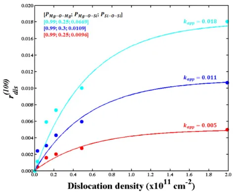
Fig 4. Contribution of dissolution rate specific to dislocations (𝒓𝒅𝒊𝒔𝒍𝒐𝒄𝒂𝒕𝒊𝒐𝒏(𝟏𝟎𝟎) ) to the total dissolution rate (𝒓⬚(𝟏𝟎𝟎)) as a function of the dislocation density. The filled circles represent the results of the different simulations and lines, the application of Eq. 16 using the parameters that allow for the best fit of all the simulations. Colors represent different [PMg-O-Mg; PMg-O-Si; PSi-O-Si] input probabilities: [0.99; 0.25; 0.0669], [0.99; 0.3; 0.0109] and
[0.99; 0.25; 0.0096] for the cyan, blue and red lines respectively. Values of kapp are 0.018, 0.011 and 0.005 for
22 3.3. Dislocation density
262
The results of simulations conducted with dislocations are reported in Fig. 4. The 263
dislocation density has been investigated by varying the surface area (i.e., all simulations were 264
conducted using a single dislocation line, while varying the simulated surface area). 265
Simulations containing dislocations have been conducted on the (100) face. The presented 266
result show the relation between the dissolution rate and the dislocation density after 267
subtraction of the “bulk” contribution to the overall dissolution rate (i.e., 𝑟( ) = 𝑟( )− 268
𝑟( )). The results highlight an asymptotic relationship between dissolution rate and 269 dislocation density. 270 271
4. Discussion
2724.1 Bulk dissolution rate evolution as a function of bond-breaking probabilities 273
From the numerical experiments described in Section 3.1, the steady state dissolution 274
rates of enstatite (defined as congruent and constant dissolution rates with time) are 275
proportional to each individual bond-breaking probability raised at a given power inferred 276
from the linear regressions depicted in a log-log diagram (Fig. 2). Moreover, since the slope 277
of the linear regression between Log(Pi) (i stands for Mg-O-Mg or Mg-O-Si or Si-O-Si) and
278
Log(r) is constant whatever the difference between the two other involved probabilities; a 279
more general function of the dissolution rate can be written as: 280 Mg O Mg Mg O Si Si O S hkl bulk k P P P i r (5)
where k is a constant and
, ,
are the corresponding slopes listed in Table 2 for the various 281regressions. The parameter k is then obtained using equation 5 and is constant for each face. 282
The different parameter values are summarized in Table 2, the
, ,
values are obtained by 28323 taking the average values of the corresponding slopes and the dissolution rates calculated with 284
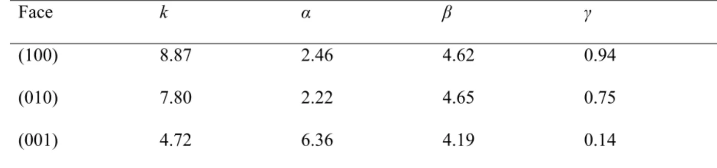
the surrogate model (Eq. 5) are compared with the simulated one in Fig. 5. 285
Face k α β γ
(100) 8.87 2.46 4.62 0.94
(010) 7.80 2.22 4.65 0.75
(001) 4.72 6.36 4.19 0.14
Table 2. Values of the different face-specific parameters of the surrogate model.
286 287
If the parameter α can be considered as constant for (100) and (010) faces (Table 1), the slope 288
that corresponds to a variation of PMg-O-Mg decreases from 7.46 to 5.05 when the difference
289
between EMg-O-Si and ESi-O-Si decreases, i.e., when EMg-O-Si gets closer to ESi-O-Si. For these
290
cases, the assumptions used in the concept of the surrogate model may not be fulfilled (e.g., k 291
is constant and does not depend on the different probabilities). This assumption will be 292
discussed in the next section. Despite this approximation and the apparent trend for the (001) 293
face, the proposed model described by Eq. 5 is capable of satisfactorily estimating the 294
simulated dissolution rates (Fig. 5) for the three different faces. Note that Eq. (5) has been 295
derived from simulations where only the first coordination sphere of surface atoms is 296
considered for expressing the dissolution probability of individual atoms. Several studies 36, 64
297
have shown that second coordination sphere may also play a role in the dissolution, and may 298
impact the shape of the developed etch pits. However, we showed that considering only the 299
first coordination sphere is enough to reproduce satisfactorily the face-specific shape of etch 300
pits observed on enstatite 41, explaining why we stick to this model in the present study.
301
Considering the impact of the second coordination sphere would make Eq. 5 more 302
sophisticated, since it would probably incorporate specific terms related to the second 303
coordination spheres. 304
24 4.2. Theoretical interpretation of the surrogate model
305
The development of the surrogate expression given in Eq. 5 is derived from a 306
statistical analysis of the outputs of the stochastic simulations of enstatite dissolution, with no 307
preconception of the mathematical form that should be used to relate the steady-state 308
dissolution rates to the individual bond-breaking probabilities describing enstatite hydrolysis. 309
In the present section, we provide a possible theoretical explanation of Eq. 5. 310
The dissolution rate can be defined as the derivative of the number of atoms that are 311
dissolved with time: 312 , M d dN r dt (6)
where NM,d stands for the amount of dissolved atoms belonging to the M species during the
313
time interval dt. Arguably, NM,d should depend on two parameters: the amount of atoms
314
located at the mineral surface (NM,S) and the intrinsic detachment rate of these atoms.
315
Importantly, classical theories of dissolution kinetics suggest that at steady-state conditions, 316
NM,S is constant and proportional to the considered surface area 6. This aspect was numerically
317
verified in our previous study 41 where we showed that the amount of surface atoms level to a
318
plateau as soon as the dissolution becomes congruent and the dissolution rate is constant. 319
At steady state, the number of dissolved atoms of Mg or Si is given by: 320
ˆ ˆ
Mg Mg Si Si
N N P N P (7)
where N is the number of dissolved atoms of Mg or Si, NˆAis the number of atoms A (Mg or
321
Si) at the mineral surface, PA is the probability that atom A is dissolved. Following the 322
previous equation, N can be rewritten as: 323
ˆ ˆ
Mg Mg Si Si
25 The dissolution of an A atom for a given coordination sphere i is given by:
324
, i i
A i A A A B
P P P (9)
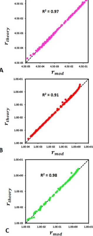
Fig 5. Comparison between the dissolution rates estimated with the surrogate model (rtheory; Eq. 5) and
dissolution rates provided by the numerical simulations (rmod) for faces (100) (A), (010) (B) and (001) (C). The
comparison is made for all the different simulations listed in Table 1. For instance, (A) presents all the simulations shown in Fig. 2, and the rate variability results from the corresponding bond-breaking probabilities that are reported in Table 1.
26 where
i and
i are the number of bonds connecting the considered A atom to another A or325
to a B atom (Si or Mg accordingly), respectively. At the solid surface, we consider that there 326
are NC different coordination spheres and ni atoms with a coordination sphere i. Therefore,
327
the probability to dissolve the atom A over the mineral face is: 328 1 1 ˆ C i i N A i A A A B i A P n P P N
and 1 ˆ NC A i i N n
(10) Or 329 1 1 ˆ C i A i A A A A A N A i A A A B A A A B A A A A B i A P n P P P P k P P N
(11) with 330 1 1 ˆ C i A i A N A i A A A B i A k n P P N
(12)and the number of dissolved atoms is: 331
ˆ ˆ
ˆ ˆ
Mg Mg Si Si
Mg Si Mg MgOMg MgOSi Si SiOSi MgOSi
Mg Mg Si Si MgOMg MgOSi SiOSi
N N N k P P k P P N k N k P P P (13) with Mg, Mg Si, Si. 332
The statistical analysis of the numerical experiments provides some values of the parameters 333
, , ,
k
(see Table 2). Surprisingly, the parameter k does not depend on the probabilities334
A A
P and PA B in the range of the numerical values used for the experiments. An appropriate 335
choice of
may explain this property. Assuming that A, A
A and j A , the j 336constant kA can be rewritten as: 337 1, 1 ˆ ˆ C i j i j N j A i A A A B i i j A A n k n P P N N
(14)27 Therefore, kA can be a constant value if
1, C i j i j N j i A A A B i i j n n P P
which is possible when 338i j
and/or i , for having positive exponents for the probabilities j PA A and/or PA B .
339
Given that the exponents are positive, considering k as a constant is a reasonable assumption 340
if the difference between PA A and PA B is significant. The validity of this condition is 341
difficult to appreciate if PA A and PA B are close, as it is the case for the simulations run for 342
(001) face (see section 4.1 and Table 1). Finally, this demonstrates that the dissolution rate is 343
therefore compatible with Eq. 5: 344 Mg O Mg Mg O Si Si O Si kP P P N r W W dt dt with 𝑊 = × × (15)
with Ncmxstanding for the number of "complexes" (see 4.4) in the enstatite cell. 345
346
4.3. Accounting for the impact of dislocation density on the dissolution rates 347
Dislocations have a measurable impact on the dissolution rate, whatever the set of 348
probabilities that was tested (Fig 6C). This result is consistent with numerical and 349
experimental studies that showed that the presence of dislocations outcropping at mineral 350
surfaces globally increases the dissolution rate when the nucleation of etch pits is 351
thermodynamically favorable (i.e., at far-from-equilibrium conditions 11, 14, 16, 23, 31, 37).
352
However, when dealing with natural samples, the dislocation density remains a parameter 353
impossible or difficult to control a priori, which complicates the prediction of its impact on 354
dissolution rate. Furthermore, several studies showed that the mineral dissolution rate is not a 355
strictly increasing function of the dislocation density 31, 37, 80 since above a given threshold, the
356
dissolution rate no longer varies with the dislocation density. 357
To qualitatively comply with the above-mentioned studies, the results for the (100) 358
face (Fig. 4) were fitted using the following empirical relation between dislocation density 359
28 and the additional dissolution rate resulting from etch pit opening at dislocation outcrop (see 360
Section 3.3.), which verifies that the dissolution rate levels to a plateau value when the 361
dislocation density tends towards infinity: 362 (100) 1 d dislocation app r k e (16)
where k and ω (≈ 5.51 x 10app 10) are empirical parameters that were obtained by calibration
363
on the outputs of the simulations, and 𝜌 is the dislocation density. Whereas ω does not seem 364
to vary with the probabilities used as input parameters, it clearly appears that k (Fig. 4) app
365
depends on the individual bond-breaking probabilities. From a physical standpoint, this 366
observation may result from the fact the first coordination spheres of atoms in the vicinity of a 367
dislocation line differ from those of atoms considered for defect-free surface. 368
Considering this apparent relationship between kapp and the probabilities, a first
369
tentative to link the global rate to the probabilities and the dislocation density was performed 370
using the same exponent for each probability as the “bulk” case. Since the global rate is 371
equivalent to 𝑟( )= 𝑟( ) + 𝑟( ), it is possible to assume the following relation: 372 1 d Mg O Mg Mg O Si Si O Si hkl dis r k k e P P P (17)
A comparison between this relation and the experimental results is given in Fig. 6A and the 373
value of kdis is given in Table 3. Although the relationship between the surrogate model and
374
the results of the simulations was proven efficient to simulate the dissolution of defect-free 375
surfaces (R² > 0.9 in all cases), it is not the case when using Eq. 17, for which R² = 0.76. 376
In order to improve the agreement between the surrogate model of the global rate and 377
the results of the simulations, numerical experiments were run for face (100) with dislocations 378
similarly to Section 4.1. The dissolution rates were fitted using the following function: 379
29
dis dis dis 1 d
Mg O Mg Mg hkl
dislocation disk P P O Si Si O SP i e
r k (18)
The values of
dis, dis, dis are lower than those obtained in the “bulk” (defect-free) case 380(Table 3), which makes sense since the coordination spheres of atoms are arguably lower in 381
the vicinity of the dislocation line, resulting in greater measured dissolution rates. 382
383
kdis dis dis disγ R2
227.9 2.46 4.62 0.94 0.72
44.7 2.09 4.09 0.67 0.86
Table 3. Values of the parameters of the model described by Eq. 17 and Eq. 18 and the correlation coefficient
384
R2. The bold characters represent the fitted parameters.
385 386
The global dissolution rate of enstatite can then be calculated by summing 𝑟( ) and 387
𝑟( ) , resulting in the following relation: 388 dis dis 1 d dis hkl di Mg O Mg Mg O Si Si O Si s Mg O Mg Mg O Si Si O Si P P r k P k P P P e (19)
Therefore, the agreement between the results of the simulations and the surrogate model is 389
improved and its correlation coefficient increases from 0.72 to 0.86 (Fig. 6B). 390
If this type of relations can be extended to other minerals and other types of defects 391
(e.g. vacancies), they may represent an interesting method to link together dissolution rates 392
derived from considerations at the atomic scale and those derived from observations at the 393
mineral scale. This type of relations can also represent a significant progress for reactive 394
transport models that simulate steady-state dissolution reactions. Indeed, even though the 395
present work represents a preliminary step to link relations at the atomic scale to macroscopic 396
dissolution rates, it shows promise as a mean to express face-specific steady-state dissolution 397
rates as a function of the bond-breaking probabilities (and therefore, of the activation energies 398
of hydrolysis) of the different types of bonds that exist for a given mineral. While some 399
studies have questioned the possibility to use the outputs of Monte Carlo simulations in 400
30 reactive-transport codes because of the limited space- and time-scales investigated following 401
such stochastic treatments of the dissolution process, here we show that steady-state 402
dissolution rates may be satisfactorily calculated from considerations at the atomic scale. As a 403
consequence, rate equations similar to Eq. 17 or Eq. 19 may be simply implemented in 404
reactive transport codes as the rate-constant of the source term of the classical reaction-405
advection-diffusion equation. This may be of interest for modeling processes for which the 406
fluid composition can be considered as unchanged over the considered simulated time, such 407
as chemical weathering in rivers or in some aquifers with a constant fluid velocity, or fluid 408
circulation in deep fractured geothermal reservoirs, where the fluid composition is 409
approximately constant and poorly affected by geothermal power plant functioning (e.g. 81).
410
More work remains however needed to assess whether this result is limited to enstatite or the 411
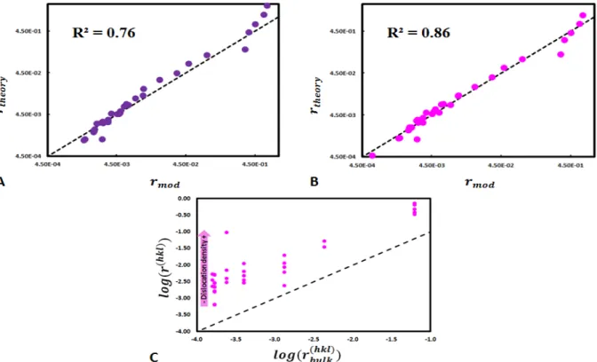
Figure 6. Comparison of experimental dissolution rates (rmod) and dissolution rates determined with the surrogate
model (rtheory) with the presence of one dislocation (dislocation density is changed by varying the surface area).
Agreement using (A) Eq. 17 and (B) Eq. 19. (C) Comparison between dislocation-driven dissolution and bulk (dislocation-free) dissolution. The presence of dislocations increases dissolution rates for all the simulations. The data points represent the simulations conducted using sets of probabilities and dislocation densities given in Table 4.
31 pyroxene group (there is a priori no reason to think so), as well as expanding the relation to 412
the transient regime, where the dissolution rate is neither stoichiometric nor constant. As long 413
as this latter task remains not fulfilled, alternate approaches such as the use of Voronoi 414
distance maps 39, 73 probably represents the most promising compromise to upscale kinetic
415
Monte Carlo simulations. This strategy nonetheless remains far more complicated than just 416
using a surrogate expression as proposed above. 417
Dislocation
density MgOMg MgOSi SiOSi
1.99E+11 0.99 0.3 0.0109 1.99E+11 0.99 0.25 0.0096 1.99E+11 0.99 0.9 0.0096 1.99E+11 0.99 0.25 0.0091 1.99E+11 0.99 0.25 0.0669 4.88E+10 0.99 0.3 0.0109 4.88E+10 0.99 0.25 0.0096 4.88E+10 0.99 0.9 0.0096 4.88E+10 0.99 0.25 0.0091 4.88E+10 0.99 0.25 0.0669 2.21E+10 0.99 0.3 0.0109 2.21E+10 0.99 0.25 0.0096 2.21E+10 0.99 0.9 0.0096 2.21E+10 0.99 0.25 0.0091 2.21E+10 0.99 0.25 0.0669 1.21E+10 0.99 0.3 0.0109 1.21E+10 0.99 0.25 0.0096 1.21E+10 0.99 0.9 0.0096 1.21E+10 0.99 0.25 0.0091 1.21E+10 0.99 0.25 0.0669 3.00E+09 0.99 0.3 0.0109 3.00E+09 0.99 0.25 0.0096 3.00E+09 0.99 0.9 0.0096 3.00E+09 0.99 0.25 0.0091 3.00E+09 0.99 0.25 0.0669 1.9899E+11 0.99 0.5 0.0096 1.9899E+11 0.8 0.3 0.0109 1.9899E+11 0.7 0.3 0.0109 4.8773E+10 0.99 0.5 0.0096 4.8773E+10 0.8 0.3 0.0109 4.8773E+10 0.7 0.3 0.0109 2.211E+10 0.99 0.5 0.0096 2.211E+10 0.8 0.3 0.0109 2.211E+10 0.7 0.3 0.0109 418
32
Table 4. Dislocation densities and probabilities used in the simulations used for Fig. 5. Bolded lines represent
419
the input parameters used in the simulations shown in Fig. 3. 420
421
4.4. Relation between the coordination of atoms leaving the surface and the 422
surrogate expression 423
Interestingly, when atoms are released from the mineral surface, they seem to have a 424
specific average coordination. This assertion is supported by the analysis of the environment 425
of Mg and Si when they leave the surface, since the mean values of Mg-O-Mg, Mg-O-Si+Mg-426
O-Si and Si-O-Si bonds remain constant and unaffected by the set of probabilities used to run 427
the simulations for all faces (see Section 3.2). However, the numerical values of the 428
parameters used in the surrogate expression of the dissolution rate are face-specific. This 429
apparent paradox can be easily explained by recalling that the histograms reported in Fig. 3 430
actually take into account all atoms leaving the surface, including those whose departure is 431
not rate-limiting of the dissolution process. 432
By analogy with Eq. 3, the surrogate expression given by Eq. 17 or Eq. 19 may reflect 433
the average coordination of atoms that control the dissolution process, as kink sites would do. 434
The fact that the numerical values of α, β and γ are face-specific indicates that this average 435
rate-controlling configuration is not unique for a given mineral. Most likely, this result 436
reflects the fact that kink sites, which are much more difficult to define using a real crystal 437
lattice than simplified isotropic cubic Kossel crystals, differ from one face to another when 438
dealing with anisotropic structures. This explanation would in turn be consistent with the 439
observed anisotropic reactivity of the pyroxene structure. 440
441
5. Conclusion
442In this study, we presented the results of hundreds of probabilistic simulations of 443
enstatite dissolution to link the overall dissolution rate to the bond-breaking probabilities used 444
33 as input parameters. By varying independently each probability, we showed that it is possible 445
to build a surrogate model that links the different probabilities to the dissolution rate 446
following a power law. This result contributes to the general effort of upscaling of mineral 447
dissolution kinetics, since this surrogate expression is based on a mechanistic approach 448
developed from considerations at the atomic-scale, from which the resulting dissolution rate 449
constants can be used as a source term in reactive transport simulations. However, the relation 450
remains valid at steady-state conditions only, and the transient regime must be treated 451
following other upscaling approaches, such as the use of Voronoï distance maps 39, 73.
452
The various simulations conducted with dislocations have shown that it is possible to 453
link the dissolution rate to the dislocation density by introducing an exponential factor to the 454
global 𝑟 = 𝑓 ∏ 𝑃 relation. This relation further extends the interest of probabilistic 455
simulations of mineral dissolution to account for the impact of some important parameters 456
that are hardly controlled in experimental studies. In addition, in case of a bond hydrolysis 457
with significant higher activation energy than the others, the dissolution rate is strongly 458
correlated to this activation energy, and the surrogate model may be used to estimate the value 459
of this parameter. 460
However, the surrogate model also presents some limitations, particularly when M-O-461
Si and Si-O-Si hydrolysis probabilities are getting close to each other (where M is a divalent 462
cation, i.e., Mg in the case of enstatite). In this specific case, the results may be out of the 463
limits of the theoretical framework that supports the development of the surrogate expression. 464
Of note, such cases are however those for which the input parameters are physically 465
unrealistic, as the activation energy of Si-O-Si hydrolysis is admitted to be much lower than 466
any other M-O-Si bond. 467
34 Finally, this study represents a first step towards the development of surrogate 468
expressions of mineral dissolution rates. Its application to natural environment, its extension 469
to other groups of minerals as well as its extension to transient state still have to be explored. 470
471
6. Acknowledgements
472A.B. thanks the University of Strasbourg for funding his PhD grant. We are also grateful for 473
the careful reviews and detailed suggestions made by two anonymous reviewers, which 474
improved an earlier version of the present paper. 475
476
7. References
4771. Berner, R. A.; Lasaga, A. C.; Garrels, R. M., The Carbonate-Silicate Cycle and Its Effect on 478
Atmospheric Carbon Dioxide over the Past 100 Millions Years. Am J Sci 1983, 284, 641-683. 479
2. Berner, R. A., A Model for Atmospheric Co2 over Phanerozoic Time. Am J Sci 1991, 291, 480
339-376. 481
3. Berner, R. A., 3GEOCARB-II - a Revised Model of Atmospheric Co2 over Phanerozoic Time. 482
Am J Sci 1994, 294, 56-91. 483
4. Berner, R. A.; Kothavala, Z., GEOCARB III: A Revised Model of Atmospheric Co2 over 484
Phanerozoic Time. Am J Sci 2001, 301, 182-204. 485
5. Lasaga, A. C., Transition State Theory. In Kinetics of Geochemical Process, Lasaga, A. C., 486
and Kirkpatrick, R.J, Ed. Mineralogical Society of America: 1981; Vol. 8, pp 135-169. 487
6. Aagaard, P.; Helgeson, H. C., Thermodynamic and Kinetic Constraints on Reaction-Rates 488
among Minerals and Aqueous-Solutions .1. Theoretical Considerations. Am J Sci 1982, 282, 237-285. 489
7. Oelkers, E. H.; Schott, J.; Devidal, J.-L., The Effect of Aluminum, Ph, and Chemical Affinity 490
on the Rates of Aluminosilicate Dissolution Reactions. Geochim Cosmochim Ac 1994, 58, 2011-2024. 491
8. Lasaga, A. C., Fundamental Approaches in Describing Mineral Dissolution and Precipitation 492
Rates. In Chemical Weathering Rates of Silicate Minerals, White, A. F.; Brantley, S. L., Eds. 493
Mineralogical Society of America: 1995; Vol. 31, pp 23-86. 494
9. Gin, S.; Jegou, C.; Frugier, P.; Minet, Y., Theoretical Consideration on the Application of the 495
Aagaard-Helgeson Rate Law to the Dissolution of Silicate Minerals and Glasses. Chem Geol 2008, 496
255, 14-24. 497
10. Luttge, A., Crystal Dissolution Kinetics and Gibbs Free Energy. Journal of Electron 498
Spectroscopy and Related Phenomena 2006, 150, 248-259. 499
11. Burch, T. E.; Nagy, K. L.; Lasaga, A. C., Free Energydependence of Albite Dissolution 500
Kinetics at 80°C and Ph 8.8. Chem Geol 1993, 105, 137-162. 501
12. Taylor, A. S.; Blum, J. D.; Lasaga, A. C., The Dependence of Labradorite Dissolution and Sr 502
Isotope Release Rates on Solution Saturation State. Geochim Cosmochim Ac 2000, 64, 2389-2400. 503
13. Beig, M. S.; Luttge, A., Albite Dissolution Kinetics as a Function of Distance from 504
Equilibrium: Implications for Natural Feldspar Weathering. Geochim Cosmochim Ac 2006, 70, 1402-505
1420. 506
35 14. Hellmann, R.; Tisserand, D., Dissolution Kinetics as a Function of the Gibbs Free Energy of 507
Reaction: An Experimental Study Based on Albite Feldspar. Geochim Cosmochim Ac 2006, 70, 364-508
383. 509
15. Dixit, S.; Carroll, S. A., Effect of Solution Saturation State and Temperature on Diopside 510
Dissolution. Geochemical Transactions 2007, 8. 511
16. Arvidson, R. S.; Luttge, A., Mineral Dissolution Kinetics as a Function of Distance from 512
Equilibrium - New Experimental Results. Chem Geol 2010, 269, 79-88. 513
17. Daval, D.; Hellmann, R.; Corvisier, J.; Tisserand, D.; Martinez, I.; Guyot, F., Dissolution 514
Kinetics of Diopside as a Function of Solution Saturation State: Macroscopic Measurements and 515
Implications for Modeling of Geological Storage of Co2. Geochim Cosmochim Ac 2010, 74, 2615-516
2633. 517
18. Nicoleau, L.; Nonat, A.; Perrey, D., The Di- and Tricalcium Silicate Dissolutions. Cement and 518
Concrete Research 2013, 47, 14-30. 519
19. Pollet-Villard, M.; Daval, D.; Ackerer, P.; Saldi, G. D.; Wild, B.; Knauss, K. G.; Fritz, B., 520
Does Crystallographic Anisotropy Prevent the Conventional Treatment of Aqueous Mineral 521
Reactivity? A Case Study Based on K-Feldspar Dissolution Kinetics. Geochim Cosmochim Ac 2016, 522
190, 294-308. 523
20. Fischer, C.; Arvidson, R. S.; Lüttge, A., How Predictable Are Dissolution Rates of Crystalline 524
Material? Geochim Cosmochim Ac 2012, 98, 177-185. 525
21. Godinho, J. R. A.; Piazolo, S.; Evins, L. Z., Effect of Surface Orientation on Dissolution Rates 526
and Topography of Caf2. Geochim Cosmochim Ac 2012, 86, 392-403. 527
22. Daval, D.; Hellmann, R.; Saldi, G. D.; Wirth, R.; Knauss, K. G., Linking Nm-Scale 528
Measurements of the Anisotropy of Silicate Surface Reactivity to Macroscopic Dissolution Rate Laws: 529
New Insights Based on Diopside. Geochim Cosmochim Ac 2013, 107, 121-134. 530
23. Smith, M. E.; Knauss, K. G.; Higgins, S. R., Effects of Crystal Orientation on the Dissolution 531
of Calcite by Chemical and Microscopic Analysis. Chem Geol 2013, 360–361, 10-21. 532
24. Wild, B.; Daval, D.; Guyot, F.; Knauss, K. G.; Pollet-Villard, M.; Imfeld, G., Ph-Dependent 533
Control of Feldspar Dissolution Rate by Altered Surface Layers. Chem Geol 2016, 442, 148-159. 534
25. Kurganskaya, I.; Luttge, A., Kinetic Monte Carlo Approach to Study Carbonate Dissolution. 535
The Journal of Physical Chemistry C 2016, 120, 6482-6492. 536
26. Daval, D.; Bernard, S.; Rémusat, L.; Wild, B.; Guyot, F.; Micha, J. S.; Rieutord, F.; Magnin, 537
V.; Fernandez-Martinez, A., Dynamics of Altered Surface Layer Formation on Dissolving Silicates. 538
Geochim Cosmochim Ac 2017, 209, 51-69. 539
27. Fischer, C.; Luttge, A., Pulsating Dissolution of Crystalline Matter. Proceedings of the 540
National Academy of Sciences 2018, 115, 897-902. 541
28. Zhang, L.; Lüttge, A., Aluminosilicate Dissolution Kinetics: A General Stochastic Model. The 542
Journal of Physical Chemistry B 2008, 112, 1736-1742. 543
29. Brantley, S. L.; Crane, S. R.; Crerar, D. A.; Hellmann, R.; Stallard, R., Dissolution at 544
Dislocation Etch Pits in Quartz. Geochim Cosmochim Ac 1986, 50, 2349-2361. 545
30. Lasaga, A. C.; Blum, A. E., Surface Chemistry, Etch Pits and Mineral-Water Reactions. 546
Geochim Cosmochim Ac 1986, 50, 2363-2379. 547
31. Lasaga, A. C.; Luttge, A., Variation of Crystal Dissolution Rate Based on a Dissolution 548
Stepwave Model. Science 2001, 291, 2400-2404. 549
32. Bouissonnié, A.; Daval, D.; Marinoni, M.; Ackerer, P., From Mixed Flow Reactor to Column 550
Experiments and Modeling: Upscaling of Calcite Dissolution Rate. Chem Geol 2018, 487, 63-75. 551
33. Amelinckx, S., The Direct Observation of Dislocations. Solid State Physics 1964. 552
34. Teng, H. H., Controls by Saturation State on Etch Pit Formation During Calcite Dissolution. 553
Geochim Cosmochim Ac 2004, 68, 253-262. 554
35. Kurganskaya, I.; Arvidson, R. S.; Fischer, C.; Luttge, A., Does the Stepwave Model Predict 555
Mica Dissolution Kinetics? Geochim Cosmochim Ac 2012, 97, 120-130. 556
36. Kurganskaya, I.; Luttge, A., A Comprehensive Stochastic Model of Phyllosilicate Dissolution: 557
Structure and Kinematics of Etch Pits Formed on Muscovite Basal Face. Geochim Cosmochim Ac 558
2013, 120, 545-560. 559