HAL Id: hal-00298479
https://hal.archives-ouvertes.fr/hal-00298479
Submitted on 6 Jul 2007HAL is a multi-disciplinary open access
archive for the deposit and dissemination of sci-entific research documents, whether they are pub-lished or not. The documents may come from teaching and research institutions in France or abroad, or from public or private research centers.
L’archive ouverte pluridisciplinaire HAL, est destinée au dépôt et à la diffusion de documents scientifiques de niveau recherche, publiés ou non, émanant des établissements d’enseignement et de recherche français ou étrangers, des laboratoires publics ou privés.
Variability in the Subtropical-Tropical Cells and its
Effect on Near-Surface Temperature of the Equatorial
Pacific: a Model Study
J. F. Lübbecke, C. W. Böning, A. Biastoch
To cite this version:
J. F. Lübbecke, C. W. Böning, A. Biastoch. Variability in the Subtropical-Tropical Cells and its Effect on Near-Surface Temperature of the Equatorial Pacific: a Model Study. Ocean Science Discussions, European Geosciences Union, 2007, 4 (4), pp.529-569. �hal-00298479�
OSD
4, 529–569, 2007 A model simulation of Pacific STC variability J. F. L ¨ubbecke et al. Title Page Abstract Introduction Conclusions References Tables Figures ◭ ◮ ◭ ◮ Back CloseFull Screen / Esc
Printer-friendly Version Interactive Discussion
EGU Ocean Sci. Discuss., 4, 529–569, 2007
www.ocean-sci-discuss.net/4/529/2007/ © Author(s) 2007. This work is licensed under a Creative Commons License.
Ocean Science Discussions
Papers published in Ocean Science Discussions are under open-access review for the journal Ocean Science
Variability in the Subtropical-Tropical
Cells and its Effect on Near-Surface
Temperature of the Equatorial Pacific: a
Model Study
J. F. L ¨ubbecke, C. W. B ¨oning, and A. Biastoch
Leibniz Institute of Marine Sciences at the University of Kiel, Germany (IfM-GEOMAR) Received: 27 June 2007 – Accepted: 2 July 2007 – Published: 6 July 2007
OSD
4, 529–569, 2007 A model simulation of Pacific STC variability J. F. L ¨ubbecke et al. Title Page Abstract Introduction Conclusions References Tables Figures ◭ ◮ ◭ ◮ Back CloseFull Screen / Esc
Printer-friendly Version Interactive Discussion
EGU
Abstract
A set of experiments utilising different implementations of the global ORCA-LIM model with horizontal resolutions of 2◦, 0.5◦and 0.25◦is used to investigate tropical and extra-tropical influences on equatorial Pacific SST variability at interannual to decadal time scales. The model experiments use a bulk forcing methodology building on the global
5
forcing data set for 1958 to 2000 developed by Large and Yeager (2004) that is based on a blend of atmospheric reanalysis data and satellite products. Whereas represen-tation of the mean structure and transports of the (sub-)tropical Pacific current fields is much improved with the enhanced horizontal resolution, there is only little difference in the simulation of the interannual variability in the equatorial regime between the 0.5◦
10
and 0.25◦model versions, with both solutions capturing the observed SST variability in the Nino3 region. The question of remotely forced oceanic contributions to the equa-torial variability, in particular, the role of low-frequency changes in the transports of the Subtropical Cells (STCs), is addressed by a sequence of perturbation experiments us-ing different combinations of fluxes. The solutions show the near-surface temperature
15
variability to be governed by wind-driven changes in the Equatorial Undercurrent. The relative contributions of equatorial and off-equatorial atmospheric forcing differ between interannual and longer, (multi-)decadal timescales: for the latter there is a significant impact of changes in the equatorward transport of subtropical thermocline water asso-ciated with the lower branches of the STCs, related to variations in the off-equatorial
20
trade winds. A conspicuous feature of the STC variability is that the equatorward trans-ports in the interior and along the western boundary partially compensate each other at both decadal and interannual time scales, with the strongest transport extrema oc-curring during El Ni ˜no episodes. The behavior is rationalized in terms of a wobbling in the poleward extents of the tropical gyres, which is manifested also in a meridional
25
OSD
4, 529–569, 2007 A model simulation of Pacific STC variability J. F. L ¨ubbecke et al. Title Page Abstract Introduction Conclusions References Tables Figures ◭ ◮ ◭ ◮ Back CloseFull Screen / Esc
Printer-friendly Version Interactive Discussion
EGU
1 Introduction
The upper-ocean circulation in the tropical Pacific can be described, in a zonally-integrated sense, in terms of shallow subtropical-tropical overturning cells (STCs; Mc-Creary and Lu,1994;Liu et al.,1994), involving equatorward geostrophic transport of water in the main thermocline, its upwelling at the equator, and return to the subtropics
5
in the surface Ekman layer (Fig.1). Since the strength of the STCs relates to the rate of supply of cold subtropical waters to the equatorial upwelling regime, low-frequency changes in STC transport have been proposed as a mechanism contributing to the modulation of sea surface temperature (SST) in the equatorial Pacific (Kleeman et al., 1999), thus representing an oceanic mechanism potentially important for generating
10
changes in tropical climate parameters, such as ENSO decadal variability (for a re-view, seeChang et al.,2006).
The dynamics of changes in STC transport and their role in equatorial SST variability have been examined by ocean model studies of various complexity and different cou-pling to the atmosphere. The original study ofKleeman et al.(1999) invoked a 312 layer
15
shallow water model coupled to a statistical atmosphere; changes in equatorial SSTs were found here to be related to changes in STC transports induced by wind stress forcing poleward of ∼23◦ latitude. The leading role of ocean dynamics in generating low-frequency equatorial SST variability was confirmed by ocean general circulation model (OGCM) results ofNonaka et al.(2002). Their set of experiments forced by
ob-20
served wind stress (from reanalysis products) showed SST anomalies at interannual time scales to be governed by equatorial (5◦N–5◦S) winds, whereas at decadal time scales both equatorial and off-equatorial winds were important; in contrast toKleeman et al. (1999) the contribution from midlatitude winds poleward of 25◦ was negligible, however. The mechanism of the off-equatorial forcing involved anomalies in heat
trans-25
port caused by a spinning up and down of the STCs, resulting in vertical shifts in the depth of the equatorial thermocline.
OSD
4, 529–569, 2007 A model simulation of Pacific STC variability J. F. L ¨ubbecke et al. Title Page Abstract Introduction Conclusions References Tables Figures ◭ ◮ ◭ ◮ Back CloseFull Screen / Esc
Printer-friendly Version Interactive Discussion
EGU et al. (1999) was presented by McPhaden and Zhang (2002); hereafter MZ02, and
McPhaden and Zhang (2004); hereafter MZ04. Estimates of meridional geostrophic transport convergence across 9◦N and 9◦S from historical hydrographic data for four time intervals of approximately 10 years, suggested a slowdown of the equatorward thermocline transport between the 1970s and the 1990s, corresponding to the
increas-5
ing trend in the central and eastern equatorial SST during this period (MZ02); during the 1990s the trend appeared to be reversed , indicating a rebound of the STCs to-wards a more active state in the early 2000s (MZ04). Sparsity of data in space and time, particularly for the western boundary current (WBC) regimes led to some uncer-tainty, however, in the calculation of the net, zonally-integrated transports (i.e., the STC
10
transports).
Understanding of the relevant processes in decadal STC variability and its relation to SST variability in the equatorial Pacific was advanced by several model studies. The importance of the WBCs in transport budgets was demonstrated by modelling studies ofLee and Fukumori(2003) (hereafter LF) andHazeleger et al.(2004), both
suggest-15
ing a tendency for a partial compensation of boundary and interior transport variability on interannual and decadal time scales. A comprehensive, three-dimensional per-spective of the structure of STC changes and of the associated phase relationships between its different branches and the equatorial SST changes was provided by Capo-tondi et al. (2005); (hereafter CA), based on an OGCM driven by observed surface
20
forcing for 1958–1997. Consistent with the observations of MZ02, the model simulated a decreasing trend for the interior thermocline transport after the mid-1970s (somewhat weaker but within the error bars of MZ02), which correlated with the SST change in the central to eastern equatorial Pacific. The interior transport variations were partially compensated, however, by boundary current changes; and an understanding of the
25
phase relationship between transport and SST changes required consideration of the ocean adjustment process through westward-propagating Rossby waves. The impor-tance of western boundary current contributions to the net equatorward transports and equatorial SST trends suggested by these studies raises the issue of possible model
OSD
4, 529–569, 2007 A model simulation of Pacific STC variability J. F. L ¨ubbecke et al. Title Page Abstract Introduction Conclusions References Tables Figures ◭ ◮ ◭ ◮ Back CloseFull Screen / Esc
Printer-friendly Version Interactive Discussion
EGU sensitivities, in particular, to horizontal resolution. Previous model studies have usually
utilized grid configurations (marginally) adapted to the minimum requirement for resolv-ing equatorial wave dynamics (e.g., a latitudinal grid spacresolv-ing near the equator of 0.6◦ in CA), but typically lacked zonal resolution to capture the western boundary regimes (e.g., zonal grid spacing in CA is 2.4◦). A first, eddy-resolving model study was reported
5
byCheng et al. (2007) for the years 1992-2003. Their simulation showed an upward trend during that period in the equatorward pycnocline transport in qualitative agree-ment with MZ04, and demonstrated the relationship between the decadal changes in the transport convergence, the EUC transport, equatorial upwelling, and SST in the equatorial Pacific. As in the previous, coarse resolution studies of LF and CA, the
10
equatorward pycnocline transports across 9◦N/9◦S in the interior Pacific were partially compensated by opposing changes in the western boundary currents. In this study, we are concerned with the interannual-decadal variations in the tropical Pacific in response to atmospheric momentum, heat and freshwater fluxes during the period 1958–2000. The atmospheric forcing builds on the formulations developed by Large and Yeager
15
(2004) based on combinations of reanalyses products and various observed fields, e.g., from satellite products. Our implementation follows the proposed configuration of “Co-ordinated Ocean-ice Reference Experiments” (COREs) by the WCRP/CLIVAR Working Group on Ocean Model Development (Griffies et al., 2007). We analyze a sequence of experiments performed with different configurations of a global ocean
cir-20
culation model (OPA9), including recent developments with 0.5◦ and 0.25◦ horizontal resolutions. The main objective of the present study is to re-examine the mechanisms of the STC variability and its relation to SST changes in the equatorial Pacific in model simulations with increased horizontal resolution, particularly in longitudinal direction. There are two specific questions we want to address: first, the relative importance
25
of equatorial vs. off-equatorial dynamic causes of low-frequency equatorial SST vari-ability; and second, the nature of the compensatory behavior between equatorward transport changes in the interior ocean and near the western boundary.
OSD
4, 529–569, 2007 A model simulation of Pacific STC variability J. F. L ¨ubbecke et al. Title Page Abstract Introduction Conclusions References Tables Figures ◭ ◮ ◭ ◮ Back CloseFull Screen / Esc
Printer-friendly Version Interactive Discussion
EGU model, describe the sequence of reference cases and perturbation experiments, and
provide a discussion of the bulk forcing methodology and its implication for the simu-lation of near-surface temperature variability. In Sect. 3 we discuss the ability of the different model configurations to capture major aspects of the annual mean flow fields in the tropical Pacific, before turning in Sect. 4 to the analysis of the low-frequency
vari-5
ability: first, in Sect. 4.1, to the variability of near-surface equatorial temperature in the Ni ˜no3-region, its relation to EUC and STC changes on interannual and decadal time scales, and the relevance of equatorial and off-equatorial atmospheric forcing; second, in Sect. 4.2, to the meridional transport variability in the interior and western boundary regimes and the degree and nature of compensation between these components. A
10
summary and conclusions are given in Sect. 5.
2 Model configurations
Three different, global implementations of the OPA ocean model (the recent release 9.0 of the model described byMadec et al.,1998) coupled to the LIM2 sea ice model (Fichefet and Morales-Marqueda,1997) are used, all utilising a tripolar grid
configura-15
tion (Madec and Imbard,1996): ORCA2, ORCA05 and ORCA025, with nominal (lon-gitudinal) grid sizes near the equator of 2◦, 0.5◦ and 0.25◦, respectively. Both higher resolution models share the same vertical grid formulation, with 46 geopotential levels of variable thickness; vertical resolution is 6 m at the surface, and there are 20 verti-cal levels in the top 500 m. In ORCA2 there are 31 vertiverti-cal levels. Vertiverti-cal mixing is
20
achieved using the TKE scheme of Blanke and Delecluse (1993). Lateral mixing is oriented along isopycnals. In ORCA2 and ORCA05 the effect of eddies is parameter-ized using a GM scheme (Gent and McWilliams,1990) with coefficients depending on the internal Rossby Radius, effectively rendering a non-eddying solution. Topographic slopes are represented by a partial step formulation (Adcroft et al., 1997); together
25
with an advanced energy-enstrophy conserving momentum advection scheme, the ORCA025-configuration was found to achieve significant improvements in simulating
OSD
4, 529–569, 2007 A model simulation of Pacific STC variability J. F. L ¨ubbecke et al. Title Page Abstract Introduction Conclusions References Tables Figures ◭ ◮ ◭ ◮ Back CloseFull Screen / Esc
Printer-friendly Version Interactive Discussion
EGU boundary current and frontal regimes in the world ocean (Barnier et al.,2006).
The momentum, heat and freshwater fluxes at the sea surface are implemented ac-cording to the “CORE” protocol, utilising the bulk forcing methodology for global ocean-ice models developed byLarge and Yeager (2004). It is based on NCEP/NCAR re-analysis products for the atmospheric state during 1958–2004, merged with various
5
observational (e.g., satellite) products for radiation, precipitation and continental run-off fields, and adjusted so as to provide a globally balanced diurnal to decadal forcing ensemble (Large,2007). A notable deviation from the reanalysis fields with some rele-vance to the present study is the correction of the low bias in NCEP wind speeds (Smith et al.,2001) by application of a spatially-dependent factor derived from the ratio of the
10
QuikScat scatterometer to the NCEP winds calculated over a two-year period (2000– 2001). The scatterometer winds are higher by 5–10% over most of the mid-latitude ocean, but the correction factor increases to more than 30 % over the equatorial Pa-cific, which can be seen in Fig. 2where a comparison between the original NCEP and the CORE zonal wind speed is shown for the equatorial region as well as for 10◦S and
15
10◦N.
A general issue of ocean-only modelling, pertinent especially to simulations of low-frequency variability, is the need to prescribe the evolution of (at least, parts of) the atmospheric state in the formulation of the surface boundary condition for tempera-ture, thereby eliminating potentially important parts of the air-sea feedback
mecha-20
nism. Specifically, this concerns the turbulent heat fluxes which can be expressed as functions of SST and atmospheric state variables (most importantly, surface air tem-perature and wind speed). For the computation of the fluxes in ocean-only models (i.e., by invoking a bulk formula), the latter have to be prescribed: since this implies a damp-ing of SST toward given surface air temperature values, SST effectively ceases to be
25
a prognostic model variable. The previous OGCM studies of the Pacific STC variabil-ity dealt with this situation in different ways: Nonaka et al. (2002) used a restoring of SST to monthly climatological values, thus allowing interannual SST variations only to be generated (albeit damped) dynamically, by changes in the wind-driven circulation.
OSD
4, 529–569, 2007 A model simulation of Pacific STC variability J. F. L ¨ubbecke et al. Title Page Abstract Introduction Conclusions References Tables Figures ◭ ◮ ◭ ◮ Back CloseFull Screen / Esc
Printer-friendly Version Interactive Discussion
EGU In contrast, both CA andCheng et al. (2007) chose bulk formulation for the turbulent
fluxes (based on different reanalysis products: NCEP for 1959–1997, and ECMWF for 1979–2003, respectively), so that the effect of interior ocean dynamics was super-imposed by the strong constraint of the surface forcing involving a relaxation toward prescribed values.
5
In the present study we basically follow the latter approach, by adopting a bulk for-mulation for the turbulent fluxes. However, we seek to gain insight into the relative importance for low-frequency SST changes of dynamical causes, such as effects of wind-driven changes in STC transports, by focusing the analysis not on the equatorial SST, but on temperature changes below the mixed layer. As shown by Fig. 3a, the
10
simulated SST (monthly time series filtered by a 23-point Hanning filter) in the Ni ˜no3 – region (150◦W to 90◦W, 5◦S to 5◦N) follows the observed variability (here taken from the COADS) rather closely, depicting the prominent temperature maxima associated with the El Ni ˜nos of 65/66, 72/73, 82/83, 91/92, and 97/98. A large fraction of the near-surface changes is also reflected at 80 m-depth (see Fig.3b). However, whereas the
15
SST is tightly constrained by the surface forcing, it will be shown below that this is not the case for the 80m-temperature (denoted as T80): i.e., perturbations of wind-driven transport can be diagnosed at 80 m, but not at the surface.
The model integrations were initialized with the annual mean temperature and salinity distributions of the Levitus climatology (Levitus et al.,1998) for low and mid-latitudes,
20
and from the data set of the Polar Hydrographic Center (PHC 2.1) for high latitudes (Steele et al., 2001). The main (reference) experiments with the interannual CORE-forcing span the period of 1958–2000. The ORCA2 and ORCA05 simulations built on a climatological spin-up of 20 years while the ORCA025 run started from scratch. These experiments with “full” interannual variation, i.e., in the momentum, heat and
25
freshwater fluxes, will be referred to as REF-2, REF-05 and REF-025, respectively. In all experiments, the freshwater forcing followed the common practice of including a relaxation of sea surface salinity to observed, climatological values. Note, however, that the restoring time scale in the subtropics-tropics is 180 days which is relatively
OSD
4, 529–569, 2007 A model simulation of Pacific STC variability J. F. L ¨ubbecke et al. Title Page Abstract Introduction Conclusions References Tables Figures ◭ ◮ ◭ ◮ Back CloseFull Screen / Esc
Printer-friendly Version Interactive Discussion
EGU weak compared to previous studies.
In order to identify the relative contributions of equatorial and off-equatorial (wind) forced circulation changes on the equatorial near-surface temperature variability, REF-05 is complemented by two pairs of perturbation experiments using ORCAREF-05. All ex-periments use the same initial conditions and span the same integration period (1958–
5
2000), but are subject to different, artificial changes in the forcing set-up; an overview is given in Table1. The first pair examines the relative importance of changes in the wind-driven circulation. In WIND, the interannual variability is restricted to the momentum fluxes (wind stress) only, while the thermohaline fluxes are based on a climatological, repeated annual cycle. In HEAT+SALT, the thermohaline fluxes are interannual, the
10
wind stress is climatological. Note that the wind speed determining thermohaline fields (e.g. evaporation) is interannually varying for HEAT+SALT and climatologically in case of WIND. The second pair aims at identifying the contribution from off-equatorial forc-ing. In EQ, the interannual (full) forcing variability is restricted to the equatorial band of 3◦S to 3◦N, whereas poleward of 7◦N/S the forcing is climatological, with a smooth
15
transition from 3◦ to 7◦latitude. Case NO EQ uses the opposite forcing configuration, i.e., interannual forcing poleward of 7◦latitude.
3 Mean circulation features
It appears useful to precede the discussion of the low-frequency variability with an inspection of the salient features of the mean subtropical-tropical circulation. Of
par-20
ticular relevance in this regard is the representation in REF-05 and REF-025 of the equatorial current system and of the western boundary current regime.
The zonally-integrated transport depicted in Fig.1for REF-05 and REF-025 exhibit the familiar signature of the subtropical-tropical overturning circulation. Specifically, in both cases one can identify the tropical cells (TCs) in the range up to 5◦N/S and 100
25
m depth in both hemispheres as well as the STCs up to 30◦S and 25◦N, respectively, and 500 m depth. The STCs span the density range of about σ0= 22.0 to 25.5 (not
OSD
4, 529–569, 2007 A model simulation of Pacific STC variability J. F. L ¨ubbecke et al. Title Page Abstract Introduction Conclusions References Tables Figures ◭ ◮ ◭ ◮ Back CloseFull Screen / Esc
Printer-friendly Version Interactive Discussion
EGU shown). The tropical cells are associated with the strong downwelling driven by the
decrease of the poleward Ekman transport around 5◦N/S (Liu et al.,1994), but they are not associated with diapycnal transports and thus, do not contribute to the ventilation of the equatorial thermocline (Hazeleger et al., 2001). The STCs involve poleward Ekman transports in the surface layer, subduction in the subtropics, and equatorward
5
geostrophic flows in the thermocline. The cells are closed by equatorial upwelling, connecting the subduction zones in the subtropics with the upwelling at the equator (Schott et al.,2004). Their mean transport in ORCA05 and ORCA025 is about 26 Sv for the northern and 39 Sv for the southern cell, slightly higher than in the companion, coarse-resolution case of REF-2. Consistent with the stronger wind stress these values
10
are higher than the ones obtained byCapotondi et al.(2005) for the NCAR model or by Hazeleger et al.(2001) in OCCAM. The asymmetry of the cell strength decreases if the overlaying deep overturning circulation is subtracted. The similarity of the meridional overturning stream function in all model versions indicates that there is only little effect of the resolution on zonally averaged transports.
15
For an examination of the equatorial current system, Fig.4provides meridional sec-tions of the mean zonal velocity at 155◦W for REF-05 and REF-025. In both cases the Equatorial Undercurrent (EUC) is centered around the equator with a core depth of about 120 m and a maximum velocity of 90 cm/s. Also the two branches of the South Equatorial Current (nSEC, sSEC), the North Equatorial Current (NEC) and the North
20
Equatorial Countercurrent (NECC) are represented well. The EUC shoals from a core depth of 200 m at the western boundary to approximately 80 m at 110◦W (not shown) and spans the density range 22.5≤σ≤26.0. This picture is in agreement with observa-tions by e.g.Wyrtki and Kilonsky(1984) andJohnson et al. (2002), except that in the ORCA05 experiments the extension of the EUC is too deep and the Subsurface
Coun-25
tercurrents (also called “Tsuchiya Jets”, Tsuchiya, 1975) are missing. The Tsuchiya Jets are, however, present in ORCA025. The Northern Subsurface Countercurrent (nSSCC), located around 4◦N with a maximum velocity of 20 cm/s is not completely separated from the EUC and NECC; the sSSCC is much weaker but discernible as a
OSD
4, 529–569, 2007 A model simulation of Pacific STC variability J. F. L ¨ubbecke et al. Title Page Abstract Introduction Conclusions References Tables Figures ◭ ◮ ◭ ◮ Back CloseFull Screen / Esc
Printer-friendly Version Interactive Discussion
EGU discrete current at 5◦S. Both currents penetrate throughout the basin, slightly diverging
towards the east as observed (Rowe et al., 2000). The higher resolution leads not only to a more realistic structure of the equatorial current system, but improves the mean transport values as well. Due to the too deep extension and the effect of the not resolved SSCCs, the EUC transport, calculated by integrating all eastward velocities
5
>5 cm/s in the density range 22.5≤σ≤26.0 between 3◦N and 3◦S, is too large in
REF-05 (34 Sv at 165◦E, 46 Sv at 155◦W and 28 Sv at 110◦W). In REF-025 the transport is about 32 Sv at 165◦E,, 38 Sv at 155◦W and 23 Sv at 110◦W which is much closer to, e.g., the direct measurements ofJohnson et al. (2002) (17 Sv at 165◦E, 35 Sv at 155◦W and 26 Sv at 110◦W), in particular in the center of the basin.
10
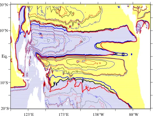
A major contribution to the zonally-integrated equatorward STC transport, and an im-portant part of the low-frequency variability examined in the next section, is provided by the current system along the western boundary. The rich structure of this system is illu-minated in Fig.5, depicting annual mean current vectors averaged between 50 m and 150 m depth in REF-05. In the northern hemisphere the NEC splits at the Philippine
15
coast, separating near 14◦N into the northwestward flowing Kuroshio and the south flowing Mindanao Current (MC,Toole et al.,1990). The MC continues along the Philip-pine Islands and turns partly into the Indonesian Throughflow (ITF), represented in the model with a mean transport of about 16 Sv, and partly into the NECC and the EUC. In the southern hemisphere the water flows to the equator along the coast of New Guinea
20
in the New Guinea Coastal Undercurrent (NGCU, e.g.Butt and Lindstrom,1994). After overshooting the equator it retroflects southeastward, feeding the EUC (Tsuchiya et al., 1989). Whereas in the models of LF and CA the western boundary currents were too weak, both the MC and the NGCU are represented well in REF-05 and REF-025, prob-ably due to better zonal resolution. For a more quantitative examination of the effect of
25
model resolution, Fig.6provides a comparative view of the WBC structure for a zonal section at 7◦S in REF-2, REF-05 and REF-025. There is a clear improvement in the representation of the New Guinea Coastal Undercurrent (NGCU) going from 2◦(which is similar to previous studies (e.g., CA) and rather typical for current climate studies)
OSD
4, 529–569, 2007 A model simulation of Pacific STC variability J. F. L ¨ubbecke et al. Title Page Abstract Introduction Conclusions References Tables Figures ◭ ◮ ◭ ◮ Back CloseFull Screen / Esc
Printer-friendly Version Interactive Discussion
EGU to 0.5◦ zonal resolution. The current is located closer to the coast and divided into
two main cores as observed (Butt and Lindstrom, 1994). The maximum meridional velocity is much higher, and the transport of the NGCU becomes more realistic: the mean transports of the western boundary currents in REF-05 are about 15 Sv in the density ranges 23.0≤σ≤26.2 across 8◦N for the MC, and 24.0≤σ≤26.7 across 6◦S for
5
the NGCU, in good agreement withLiu and Philander(2001) andSloyan et al.(2003), respectively. In ORCA2 the currents are much weaker with a transport of about 13 Sv (MC) and 9 Sv (NGCU). In contrast, further increase in resolution to 0.25◦ does not lead to significant changes in either the wbc structures or transports.
4 Interannual – decadal variability 10
The low-frequency variability behavior of the model solutions is diagnosed on the basis of monthly-mean output fields, smoothed either by a 23-point Hanning filter to remove intraseasonal variability (in the following referred to as “interannual smoothing”), or on a 119-point (∼10 years) Hanning filter (“decadal smoothing”).
4.1 Equatorial near surface temperature (NST) and STC transport
15
We begin with an inspection of the equatorial near surface temperature (NST) vari-ability, followed by assessing its relation to wind-driven, equatorial and off-equatorial, changes in the EUC, and in turn, the STC transports. A first result to be noted con-cerns the sensitivity to model resolution: comparison of the variability signatures in the reference cases REF-05 and REF-025 reveals only minor differences (Fig. 7a);
20
we shall thus focus our analysis on the sequence of experiments (i.e., reference case and perturbation experiments) conducted with the ORCA05-configuration. Figure7b compares the variability of T80 in the reference case REF-05 with the result of the per-turbation experiments WIND and HEAT+SALT. Obviously, the variability of T80 can be
explained nearly completely as a dynamic effect of the wind forcing, both for the
OSD
4, 529–569, 2007 A model simulation of Pacific STC variability J. F. L ¨ubbecke et al. Title Page Abstract Introduction Conclusions References Tables Figures ◭ ◮ ◭ ◮ Back CloseFull Screen / Esc
Printer-friendly Version Interactive Discussion
EGU inating, interannual (ENSO) time scale as well as for its decadal modulation. Note
that (not shown here) the behavior is different for the SST which is more tightly con-strained by the surface heat flux formulation. The significant influence of changes in the wind-driven circulation is illustrated in Fig. 7c: the NST-anomalies in the eastern equatorial region are closely related to the EUC transport variability; both time series
5
(interannually smoothed) are strongly anti-correlated (r=–0.91), emphasizing the key role of the eastward transport and upwelling of subtropical waters by the EUC (as, e.g., discussed bySloyan et al.,2003, and demonstrated explicitly in the model analysis of Cheng et al.,2007).
What is the relative importance for the equatorial NST variability of atmospheric
forc-10
ing within the equatorial regime vs. off-equatorial forcing variability over the tropical Pacific? This question, previous addressed in the study of Nonaka et al. (2002), is re-visited here with the perturbation experiments EQ and NO EQ (see Table 1). A first look at the EUC transport time series in these experiments (not shown) reveals roughly equal contributions to the variance of interannual variability by the equatorial
15
and the off-equatorial forcing (however, with strong variations in the ratio between the two components during the four decades of the integration); the transport anomalies in EQ and NO EQ add almost linearly to the transport anomalies of the reference exper-iment REF-05. Figure8shows time series of T80 anomalies averaged over the Ni ˜no3
region from the experiments REF-05, EQ and NO EQ, revealing a distinctive difference
20
in the relative importance of off-equatorial forcing mechanisms between interannual and decadal time scales. At interannual time scales the NST appears mainly driven by the equatorial forcing, although there are some minor in-phase variations also in the NO EQ run. About 70% of the interannual variability of the reference experiment can be explained by equatorial forcing while the off-equatorial forcing accounts for around
25
30%. At decadal time scale the variations in the NO EQ experiment are of the same order as in the EQ run, consistent with the results ofNonaka et al. (2002). The ratio between equatorial and off-equatorial influence changes to 50% : 50%.
thermo-OSD
4, 529–569, 2007 A model simulation of Pacific STC variability J. F. L ¨ubbecke et al. Title Page Abstract Introduction Conclusions References Tables Figures ◭ ◮ ◭ ◮ Back CloseFull Screen / Esc
Printer-friendly Version Interactive Discussion
EGU cline water on the equatorial temperature variability, i.e., the mechanism proposed by
Kleeman et al. (1999), we define an index for the STC strength (following Lohmann and Latif,2005), based on the sum of the transport maxima of the northern and south-ern cells in the latitude range 8◦–12◦(for the monthly time series of the model output). Figure9a shows the interannual variability of that index for REF-05, as well as for the
5
EQ and NO EQ experiments. In contrast to the behavior of the tropical cells (TCs) discussed by Lohmann and Latif (2005), the STC variability is mainly driven by off-equatorial forcing, closely related (not shown) to the Ekman transports associated with the zonal wind stress variability at these latitudes. The relation between the STC trans-port variability and the near-surface equatorial temperature is examined in Fig.9b and
10
c. It indicates a similar difference for the role of the STC variability between interannual and decadal time scales as found for the equatorially and off-equatorially forced EUC transport variability: while there is only a weak relation between interannual STC and NST changes (r=-0.27) as well as between STC and EUC anomalies (not shown), the wind-driven STC changes on decadal time scales appear clearly linked to the EUC
15
and NST; the correlation between the decadally smoothed STC index and the Ni ˜no3
T80 is r=–0.92 in the NO EQ experiment and almost that high in REF-05. This
con-nection between STC, EUC and SST changes at decadal time scales was also shown by Cheng et al. (2007) who found the increase in the meridional volume transport convergence in the 1990s to be accompanied by a higher EUC transport and
anoma-20
lous upwelling. The model solutions thus suggest that the part of the NST variability which was found to be associated with off-equatorial atmospheric forcing, especially at decadal time scales, can be rationalized in terms of the variability in equatorward transport of subtropical thermocline waters with the subsurface STC branches which, in turn, are related to the variability in the off-equatorial trade winds.
25
4.2 Interior vs. WBC transport variability
As emphasized in the model study of CA, a quantitative assessment of the phase relationship between the equatorward transports of thermocline water and the
equa-OSD
4, 529–569, 2007 A model simulation of Pacific STC variability J. F. L ¨ubbecke et al. Title Page Abstract Introduction Conclusions References Tables Figures ◭ ◮ ◭ ◮ Back CloseFull Screen / Esc
Printer-friendly Version Interactive Discussion
EGU torial variability requires a rather detailed examination of the different STC branches
contributing to the zonally-integrated index. A dissection of the temporal evolution of the three-dimensional current fields as provided by CA is not repeated here; however, Fig. 10 provides a view in a complementary, statistical sense of the thermocline ar-eas where the main contributions to the meridional transports are concentrated. The
5
strongest signal is clearly found in a narrow band along the western boundary, remi-niscent of the dominant role of the western boundary window in the mean STCs (as shown, e.g. in transport calculations byHuang and Liu,1999). The interior variability signal is not spread across the longitudinal extent of the basin, but rather concentrated in wedges in the central Pacific, consistent with the accumulated transport integration
10
byCheng et al.(2007). Concerning the latitudinal extent, there seems to be no direct meridional flow to the equator, especially in the northern hemisphere, which is likely to be related to the potential vorticity ridge (Rothenstein et al., 1997; Johnson and McPhaden,1999). Maxima are found in the latitude ranges of the zonal currents (see Fig.4) known to contribute to the interior exchange window, i.e., the branches of the
15
South Equatorial Current (SEC) around 3◦ to 4◦N/S as well as the North Equatorial Current (NEC) at 12◦to 15◦N.
Calculating the net equatorward transport in the density range of the STC (22.7 ≤
σ ≤26.8 for the southern and 22.7≤σ≤26.5 for the northern cell, only considering the flow below 50 m depth, i.e, below the surface layer dominated by the Ekman
trans-20
port) averaged over 6◦S to 10◦S and 6◦N to 10◦N, respectively, results in time mean transports of 14.8 Sv (14.1 Sv) at the western boundary and 9.7 Sv (6.8 Sv) in the in-terior in the southern (northern) hemisphere. The separation longitude between WBC and INTERIOR is chosen to be at 160◦E (southern hemisphere) and 145◦E (north-ern hemisphere) in order to include possible tight recirculation cells of the west(north-ern
25
boundary currents in the WBC part and consistent with the interior range as defined in the observational study of MZ02. The mean structure and transport values, as well as the interannual variability of the WBC strength are rather similar in ORCA05 and ORCA025, but significantly different from ORCA2. Figure11shows transport time
se-OSD
4, 529–569, 2007 A model simulation of Pacific STC variability J. F. L ¨ubbecke et al. Title Page Abstract Introduction Conclusions References Tables Figures ◭ ◮ ◭ ◮ Back CloseFull Screen / Esc
Printer-friendly Version Interactive Discussion
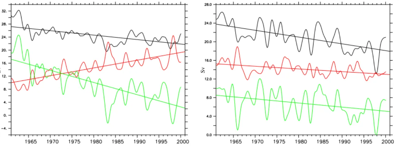
EGU ries for the western boundary and interior branches. For the southern cell, interior and
western boundary transports are highly anticorrelated both at interannual and decadal time scales, in agreement with LF and CA. The linear correlation coefficient is about r=–0.92 for the interannually smoothed time series. The overall decline of the STC strength is governed by a transport change in the interior and partly compensated by
5
a rise in the strength of the NGCU. Using the definition by LF the (interannual) degree of compensation is about C=56%.
In the northern hemisphere, the situation for the longer time scales is different: whereas the INTERIOR transport variability is partially compensated by the WBC on interannual time scales (r=–0.72), there is no such tendency for the overall trends at
10
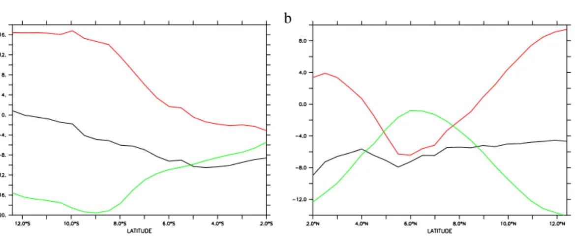
10◦N, in apparent contrast to the results of LF. However, inspection of the latitudinal dependence of the WBC and INTERIOR transports indicates that time series evaluated at single sections have to be interpreted with caution. This is demonstrated in Fig.12 for the linear trends of the STC transports and their components. In the southern hemi-sphere, the overall, net decline in the STC transport gradually fades with increasing
15
poleward latitude, while the trends in both the INTERIOR (of the same sign as the to-tal) and the WBC components (of opposite sign) strongly increase and attain maximum values at about 10◦S. The latitudinal dependence is even more complex for the north-ern STC where the individual components go through a distinct minimum at around 6◦N.
20
At interannual time scales it is striking that both in the northern and the southern hemisphere, the strongest extrema of WBC and INTERIOR occur in El Ni ˜no years (e.g. 1965/1966, 1982/1983, 1997/1998) which is not the case for the total STC trans-port. During an El Ni ˜no event the equatorward transport within the STCs becomes stronger at the western boundary, but weaker in the interior. This behavior can be
25
rationalized in terms of changes in the horizontal circulation, i.e., in the poleward ex-tension of the tropical gyres which encompass net, vertically-integrated equatorward flows at the western boundary and net poleward flows in the interior (Fig.5a). Com-parison of the gyre patterns between El Ni ˜no and La Ni ˜na phases exhibit little changes
OSD
4, 529–569, 2007 A model simulation of Pacific STC variability J. F. L ¨ubbecke et al. Title Page Abstract Introduction Conclusions References Tables Figures ◭ ◮ ◭ ◮ Back CloseFull Screen / Esc
Printer-friendly Version Interactive Discussion
EGU in maximum gyre transports, but considerable changes in the poleward extension of
the gyres in the western part of the ocean basin; specifically, the bifurcation latitudes between poleward and equatorward flows at the western boundary vary by 3.5◦ (2.5◦) for the northern (southern) tropical gyre, with a poleward shift during El Ni ˜no phases. A variation in the northern bifurcation latitudes and its implications have previously been
5
discussed byKim et al. (2004) in a high resolution ocean model study, noting an in-crease in the flow of NEC water into the MC during El Ni ˜no years when the bifurcation was found to shift to a more northerly position.
The expansion and contraction of the poleward extent of the tropical gyres implies that over certain latitude bands, even without a change in the maximum gyre
trans-10
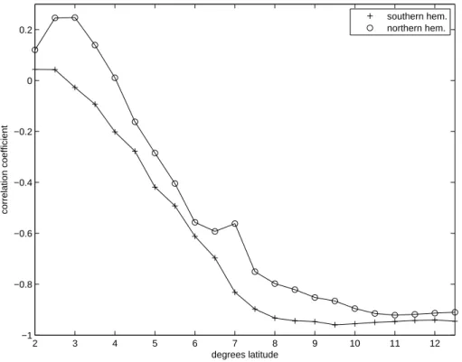
ports, there will be a variation in the transport of the western boundary currents, com-pensated by opposite changes in interior meridional transports. More generally, the behavior suggests that this may be a possibly important, overlooked mechanism for the conspicuous compensation between wbc and interior transport changes: it offers a simple rationale for the strong, non-lagged anticorrelation noted here and in previous
15
model studies, as well as for the poleward increase in the individual components. An additional feature that may be attributed to this mechanism, is that the highest anticor-relations between WBC and INTERIOR transports are located in the latitude ranges most strongly affected by a wobbling of the tropical gyres, i.e., in the transition region between the tropical and subtropical gyres: the correlation values (with zero lag) on
20
interannual time scales (i.e., based on detrended interannually filtered, monthly time series) are depicted in Fig.14; they show a high degree of anticorrelation poleward of about 6◦- 8◦ latitude, gradually decreasing towards the equator in both hemispheres.
Similar changes in the poleward gyre extent also appear as a characteristic of the decadal variability. Figure 5b provides a comparison of the barotropic stream
func-25
tions for the decades 1961–1970 and 1981–1990. Whereas differences in the north-ern hemisphere appear relatively weak, the bifurcation latitude of the SEC exhibits a prominent shift to the south from the first to the second period, consistent with the in-creasing NGCU and dein-creasing interior transports noted above. These patterns, and
OSD
4, 529–569, 2007 A model simulation of Pacific STC variability J. F. L ¨ubbecke et al. Title Page Abstract Introduction Conclusions References Tables Figures ◭ ◮ ◭ ◮ Back CloseFull Screen / Esc
Printer-friendly Version Interactive Discussion
EGU their similarity to the behavior on interannual time scales, suggest that the
compen-satory character of meridional transport changes at the boundary and in the interior may be rationalized in a different way than previously proposed: the present analy-sis suggests that in addition to variations in the strength of the tropical gyre (i.e., the mechanism invoked by LF), or to the adjustment of the ocean by westward propagating
5
Rossby waves invoked by CA, a wobbling of the poleward extent of the tropical gyres and concomitant changes in the bifurcation latitudes of the NEC and SEC flows have to be considered as key factors.
5 Summary and discussion
In this study the question of remotely forced contributions to the temperature variability
10
in the equatorial Pacific, i.e. the possible role of low-frequency changes in the transport of the STCs, was addressed in model simulations utilizing different implementations of the global ORCA-LIM model, forced by recently developed atmospheric forcing fields based on modified reanalysis products for the period 1958 to 2000.
Our sequence of experiments included model versions with horizontal meshes
vary-15
ing from coarse, non-eddy resolving (2◦ and 0.5◦) to eddy-permitting (0.25◦), the latter permitting a much improved representation of both the zonal equatorial current struc-ture (e.g., with an emergence of Tsuchiya Jets) and of the western boundary currents (where significant changes occurred between the 2◦and 0.5◦simulations, but compar-atively minor ones between 0.5◦and 0.25◦). In contrast to the resolution dependencies
20
of the mean current structures and transports, the model solutions revealed relatively little sensitivity of the low-frequency variability in equatorial SST; more specifically, both the 0.5◦- and 0.25◦-simulations closely reproduced the observed SST variability in the Ni ˜no3-region. Further investigation of the mechanisms involved in this variability was thus based mainly on two sets of 0.5◦ – experiments with different, artificial
perturba-25
tions in the atmospheric forcing: one set aiming at an isolation of the effect of wind-driven circulation changes; the other set re-visiting the issue of the relative
contribu-OSD
4, 529–569, 2007 A model simulation of Pacific STC variability J. F. L ¨ubbecke et al. Title Page Abstract Introduction Conclusions References Tables Figures ◭ ◮ ◭ ◮ Back CloseFull Screen / Esc
Printer-friendly Version Interactive Discussion
EGU tions of equatorial vs. off-equatorial (i.e., equatorward and poleward of about 5◦N/S)
atmospheric forcing.
The solutions confirmed previous model suggestions of a significant influence of off-equatorial, wind driven changes on the low-frequency, near surface temperature variability in the equatorial Pacific. Particular findings are:
5
– interannual-decadal equatorial temperature variability is tightly related to the EUC
transport, and nearly completely explained as an effect of wind-driven changes in the tropical circulation;
– the variability at interannual (ENSO) time scales is predominantly governed by
near-equatorial wind forcing, whereas a significant part of the variability on
10
decadal time scales (i.e., about 50% of the variance over the integration period) is related to off-equatorial forcing, and thus, to changes in the equatorward transport of subtropical thermocline water as characterized by the strength of the northern and southern hemisphere STCs;
– the net changes in STC transport involve much larger changes in the interior 15
and WBC transport, which partially compensate each other at both decadal and interannual time scales, with transport extrema (i.e., maximum equatorward ther-mocline transport in the interior) coinciding with El Ni ˜no episodes.
The interpretation of variability features obtained from ocean model simulations sub-ject to a prescribed atmospheric state has to account for at least two issues: the
ef-20
fect of compromising potentially important feedback mechanisms in air-sea interaction, and possible errors in the prescribed atmospheric fields. With respect to the former, the main choice for ocean modelling studies has been the use of bulk formulations for the sensible and latent air-sea heat fluxes (including the use of linearized expressions, such as proposed byBarnier et al.,1995 or, originally, by Haney,1971). An
alterna-25
tive for modelling studies specifically of the ocean’s response to variable wind stresses (for example,Hazeleger et al.,2004) has been coupling to an atmospheric mixed-layer
OSD
4, 529–569, 2007 A model simulation of Pacific STC variability J. F. L ¨ubbecke et al. Title Page Abstract Introduction Conclusions References Tables Figures ◭ ◮ ◭ ◮ Back CloseFull Screen / Esc
Printer-friendly Version Interactive Discussion
EGU model. The present forcing configuration involves a rather comprehensive bulk
formu-lation for the thermal forcing, following recent design considerations for “Coordinated Ocean-ice Reference Experiments” (CORE,Griffies et al., 2007), using atmospheric state data developed byLarge and Yeager(2004) based on adjusted NCEP/NCAR re-analysis products (see also Large, 2007). As in the model studies of CA andCheng
5
et al. (2007) this implies a damping of SST toward given values, so that SST effectively becomes a diagnostic rather than prognostic variable, rendering it rather useless for diagnosing effects of ocean dynamics. In order to identify, at least qualitatively, dy-namical influences on SST,Nonaka et al.(2002) chose a climatological thermal forcing (i.e., a restoring of SST to monthly-mean values), allowing interannual SST changes
10
only to be generated (albeit damped) by either equatorial or off-equatorial wind-forced changes in the upper-layer circulation.
In the present study we chose an alternative approach, by not considering the vari-ability of SST, but of the temperature below the mixed layer (at 80 m depth): in the reference experiments with interannual variability in both thermal and wind forcing, this
15
near-surface temperature (NST) closely followed the SST variability; however, com-pared to the SST, the NST was found much less constrained by the local thermal forc-ing, thus allowing to diagnose effects of wind-driven transport variability. The presence of a significant effect on decadal NST variability by lateral transport changes associated with the strength of the STCs is complementary to previous model results: to the study
20
of Nonaka et al. (2002) who showed a response of equatorial SST to decadal STC variability forced by off-equatorial trade wind variations (against the damping of the lo-cal (in their case, climatologilo-cal) heat fluxes); and to the study ofCheng et al.(2007) who demonstrated the leading role of an increasing STC strength for the cooling of the equatorial Pacific after the mid-1990s, against the heating effect of the surface heat
25
flux anomalies during that period.
With respect to possible biases in the atmospheric state data the main concern, in a study of forced tropical variability, has to be the accuracy of surface wind products and computation of wind stress. The CORE forcing involves a correction of known
bi-OSD
4, 529–569, 2007 A model simulation of Pacific STC variability J. F. L ¨ubbecke et al. Title Page Abstract Introduction Conclusions References Tables Figures ◭ ◮ ◭ ◮ Back CloseFull Screen / Esc
Printer-friendly Version Interactive Discussion
EGU ases in NCEP winds using adjustments derived from comparison with satellite vector
winds from QSCAT (Large and Yeager,2004). A potential problem not affected by that correction is the presence of artificial trends in the wind fields: comparison by Alory et al. (2005) of an (ORCA2-) model simulation with sea level data revealed a spurious trend in the Pacific trade winds before the mid-1970s, implying that the simulated
de-5
cline in the STC strength during that period involves a strong artificial component. This was also demonstrated bySchott et al.(2007) who showed that the large decreasing trends in the tropical Ekman divergence resulting from NCEP/NCAR wind stresses as well as in the interior STC transport convergence are significantly reduced in GECCO assimilation results which involved an adjustment of wind stress as a key part of the
10
minimization of model – data misfits. According to these studies the absolute trends in STC strength components, obtained in the present model solution, of –14.5 Sv (– 3.5 Sv) in the interior and +9.5 Sv (–2.5 Sv) at the western boundary for the southern (northern) cell are likely to be overestimated.
Irrespective of possible biases in the quantitative simulation of multi-decadal changes
15
in the tropical circulation, especially during periods before the mid-1970s, the present sequence of ocean model experiments provides a viable basis for elucidating the mech-anisms governing this variability. This holds in particular for the conspicuous partial compensation of equatorward thermocline transport changes in the ocean interior and western boundary currents which has repeatedly been noted in previous studies and
20
is replicated in the present simulations. Within the southern cell the interior and WBC transport changes are anticorrelated at decadal as well as at interannual (and even, not examined further in this study, seasonal) time scales, while there is no decadal compensation within the northern cell. Additionally, in contrast to the total STC trans-port, the WBC and interior transport variations are found to be correlated with ENSO:
25
during an El Ni ˜no event, when the transport of the EUC is weak due to the relaxation of the trade winds, the equatorward transport within the STCs is stronger at the western boundary, but weaker in the interior. This indicates that while the time-mean transport is concentrated in the WBC, the variability of the interior transport may be more important
OSD
4, 529–569, 2007 A model simulation of Pacific STC variability J. F. L ¨ubbecke et al. Title Page Abstract Introduction Conclusions References Tables Figures ◭ ◮ ◭ ◮ Back CloseFull Screen / Esc
Printer-friendly Version Interactive Discussion
EGU in determining the EUC transport, and thus, the eastern equatorial NST variations.
Pre-vious explanations for the anticorrelation between WBC and interior transport changes involved the spinning up and down of the tropical gyre circulation in response to varia-tions in wind stress curl (LF) and the adjustment of the ocean by westward propagating Rossby waves (CA). Our analysis also suggests an explanation in terms of variations
5
in the tropical gyres; however, in contrast to the interpretation of LF, the main reason for the tight anti-correlation on both interannual (ENSO) and (multi-)decadal time scales appears to be a variation in the poleward extension of the tropical gyres.
References
Adcroft, A., Hill, C., and Marshall, J.: Representation of topography by shaved cells in a height 10
coordinate ocean model, Mon. Wea. Rev., 125, 2293–2315, 1997. 534
Alory, G., Cravatte, S., Izumo, T., and Rodgers, K. B.: Validation of a decadal OGCM simulation for the tropical pacific, Ocean Modelling, 10, 272–282, 2005. 549
Barnier, B., Siefridt, L., and P., M.: Thermal forcing for a global ocean circulation model using a three-year climatology of ECMWF analyses, J. Marine Systems, 6(4), 363–380, 1995.547 15
Barnier, B., Madec, G., Penduff, T., Molines, J.-M., Treguier, A.-M., Beckmann, A., Biastoch, A., B ¨oning, C., Dengg, J., Gulev, S. Le Sommer, J., Remy, E., Talandier, C., Theetten, S., and Maltrud, M.: Impact of partial steps and momentum advection schemes in a global ocean circulation model at eddy permitting resolution, Ocean Dynamics, 56(5–6), 543–567, 2006. 535
20
Blanke, B. and Delecluse, P.: Variability of the tropical Atlantic ocean simulated by a general circulation model with two different mixed layer physics, J. Phys. Oceanogr., 23, 1363–1388, 1993. 534
Butt, J. and Lindstrom, E.: Currents off east coast of New Ireland, Papua-New Guinea and their relevance to regional undercurrents in the western equatorial Pacific Ocean, J. Geo-25
phys. Res., 99, 12 503–12 514, 1994. 539,540
Capotondi, A., Alexander, M. A., Deser, C., and McPhaden, M. J.: Anatomy and Decadal Evolution of the Pacific Subtropical-Tropical Cells (STCs), J. Climate, 18(18), 3739–3758, 2005. 532,538
OSD
4, 529–569, 2007 A model simulation of Pacific STC variability J. F. L ¨ubbecke et al. Title Page Abstract Introduction Conclusions References Tables Figures ◭ ◮ ◭ ◮ Back CloseFull Screen / Esc
Printer-friendly Version Interactive Discussion
EGU
Chang, P., Yamagata, T., Schopf, P., Behera, S. K., Carton, J., Kessler, W. S., Meyers, G., Qu, T., Schott, F., Shetye, S., and Xie, S. P.: Climate Fluctuations of Tropical Coupled Systems – The Role of Ocean Dynamics, J. Climate, 19, 5122–5174, 2006.531
Cheng, W., McPhaden, M. J., Zhang, D., and Metzger, E. J.: Recent Changes in
the Pacific Subtropical Cells Inferred from an Eddy-Resolving Ocean Circulation Model, 5
J. Phys. Oceanogr., 37, 1340–1356, 2007.533,536,541,542,543,548
Fichefet, T. and Morales-Marqueda, M. A.: Sensitivity of a global sea ice model to the treatment of ice thermodynamics and dynamics, J. Geophys. Res., 102, 12 609–12 646, 1997. 534
Gent, P. R. and McWilliams, J.: Isopycnal mixing in ocean circulation models,
J. Phys. Oceanogr., 20, 150–156, 1990. 534 10
Griffies, S., B ¨oning, C. W., and Treguier, A. M.: Design Considerations for Coordinated Ocean - Ice Reference Experiments, WGSF/WCRP Flux News, 3, 3–5, 2007.533,548
Haney, R. L.: Surface Thermal Boundary Condition for Ocean Circulation Models, J. Phys. Oceanogr., 1(4), 241–248, 1971. 547
Hazeleger, W., de Vries, P., and van Oldenbourgh, G. J.: Do tropical cells ventilate the Indo-15
Pacific equatorial thermocline?, Geophys. Res. Lett., 28(9), 1763–1766, 2001.538
Hazeleger, W., Seager, R., Cane, M., and Naik, N. H.: How can tropical Pacific ocean heat transport vary?, J. Phys. Oceanogr., 34, 320–333, 2004.532,547
Huang, B. and Liu, Z.: Pacific subtropical–tropical thermocline water exchange in the National Centers for Environmental Prediction ocean model, J. Geophys. Res., 104(C5), 11 065– 20
11 076, 1999.543
Johnson, G. C. and McPhaden, M.: Interior Pycnocline Flow from the Subtropical to the Equa-torial Pacific Ocean, J. Phys. Oceanogr., 29(12), 3073–3089, 1999. 543
Johnson, G. C., Sloyan, B. M., Kessler, W. S., and McTaggert, K. E.: Direct measurements of upper ocean currents and water properties across the tropical pacific during the 1990s, 25
Progr. Oceanogr., 52, 31–61, 2002. 538,539
Kim, Y. Y., Qu, T., Jensen, T., Miyahima, T., Mitsudera, H., Wang, H.-W., and Ishida, A.: Seasonal and interannual variations of the North Equatorial Current bifurcation in a high-resolution OGCM, J. Geophys. Res., 109, C03040, doi:10.1029/2003JC002013., 2004.545 Kleeman, R., McCreary, J. P., and Klinger, B. A.: A mechanism for generating ENSO decadal 30
variability, Geophys. Res. Lett., 26(12), 1743–1746, 1999. 531,542
Large, W. and Yeager, S.: Diurnal to decadal global forcing for ocean and sea-ice models: the data sets and flux climatologies, NCAR Technical Note: NCAR/TN–460+STR, CGD Division
OSD
4, 529–569, 2007 A model simulation of Pacific STC variability J. F. L ¨ubbecke et al. Title Page Abstract Introduction Conclusions References Tables Figures ◭ ◮ ◭ ◮ Back CloseFull Screen / Esc
Printer-friendly Version Interactive Discussion
EGU
of the National Center for Atmospheric Research, 2004.533,535,548,549
Large, W. G.: Core Forcing for Coupled Ocean and Sea - Ice Models, WGSF/WCRP Flux News, 3, 2–3, 2007. 535,548
Lee, T. and Fukumori, I.: Interannual-to-decadal variations of the tropical-subtropical exchange in the Pacific Ocean: Boundary versus interior pycnocline transports, J. Climate, 16, 4022– 5
4042, 2003. 532
Levitus, S., Boyer, T. P., Conkright, M. E., O’Brian, T., Antonov, J., Stephens, C., Stathopolos, L., Johnson, D., and Gelfeld, R.: World Ocean Database 1998, NOAA Atlas NESDID18, 1998. 536
Liu, Z. and Philander, G.: Tropical-extratropical oceanic exchange pathways, in: Ocean Circula-10
tion and Climate: Observing and Modeling the Global Ocean, edited by Siedler, G., Church, J., and Gould, J., pp. 247–257, Academic Press, 2001.540
Liu, Z., Philander, S. G. H., and Pacanowski, R. C.: A GCM Study of Tropical-Subtropical Upper-Ocean Water Exchange, J. Phys. Oceanogr., 24, 2606–2623, 1994. 531,538 Lohmann, K. and Latif, M.: Tropical Pacific Decadal Variability and the Subtropical-Tropical 15
Cells, J. Climate, 18, 5136–5178, 2005.542
Madec, G. and Imbard, M.: A global ocean mesh to overcome the North Pole singularity, Clim. Dyn., 12, 381–388, 1996. 534
Madec, G., Delecluse, P., Imbard, M., and Levy, C.: OPA 8.1 general circulation model reference manual, Notes de l’IPSL, Universit ´e P. et M. Curie, B102 T15-E5, 4 place Jussieu, Paris 20
cedex 5, N◦S 11, 91p., 1998. 534
McCreary, J. P. and Lu, P.: Interaction between the Subtropical and Equatorial Ocean Circula-tions: The Subtropical Cell, J. Phys. Oceanogr., 24, 466–496, 1994. 531
McPhaden, M. J. and Zhang, D.: Slowdown of the meridional overturning circulation in the upper Pacific Ocean, Nature, 415, 603–608, 2002. 532
25
McPhaden, M. J. and Zhang, D.: Pacific Ocean circulation rebounds, Geophys. Res. Lett., 31, L18301, doi:10.1029/2004GL020727, 2004. 532
Nonaka, M., Xie, S.-P., and McCreary, J.: Decadal variations in the Subtropical Cells and equatorial Pacific SST, Geophys. Res. Lett., 29(7), 20–1–20–3, 2002.531,535,541,548 Rothenstein, L. M., Zhang, R.-H., Busalacchi, A., and Chen, D.: A Numerical Simulation of the 30
Mean Water Pathways in the Subtropical and Tropical Pacific Ocean, J. Phys. Oceanogr., 28(2), 322–343, 1997. 543
OSD
4, 529–569, 2007 A model simulation of Pacific STC variability J. F. L ¨ubbecke et al. Title Page Abstract Introduction Conclusions References Tables Figures ◭ ◮ ◭ ◮ Back CloseFull Screen / Esc
Printer-friendly Version Interactive Discussion
EGU
Velocity, Transport, and Potential Vorticity, J. Phys. Oceanogr., 30, 1172–1187, 2000.539 Schott, F., Wang, W., and Stammer, D.: Variability of Pacific subtrobical cells in the 50-year
ECCO assimilation, Geophys. Res. Lett., 34, L05604, doi:10.1029/2006GL02847, 2007.549 Schott, F. A., Creary, J. P. M., and Johnson, G.: Shallow overturning circulation of the tropical-subtropical oceans, in: Earth Climate: The Ocean-Atmoshere Interaction, edited by Wang, 5
C., Xie, S.-P., and Carton, J. A., pp. 261–304, American Geophysical Union, 2004.538 Sloyan, B. M., Johnson, G. C., and Kessler, W. S.: The Pacific Cold Tongue: A Pathway for
Interhemisheric Exchange, J. Phys. Oceanogr., 33(5), 1027–1043, 2003. 540,541
Smith, S. R., Legler, D. M., and Verzone, K. V.: Quantifying Uncertainties in NCEP Reanalysis Using High-Quality Research Vessel Observations, J. Climate, 14, 4062–4072, 2001. 535 10
Steele, M., Morley, R., and Ermold, W.: PHC: A Global Ocean Hydrography with a High-Quality Arctic Ocean, J. Climate, 14(9), 2079–2087, 2001.536
Toole, J. M., Millard, R. C., Wang, Z., and Pu, S.: Observations of the Pacific North Equatorial Current bifurcation at the Philippine coast, J. Phys. Oceanogr., 20, 307–318, 1990.539 Tsuchiya, M.: Subsurface countercurrents in the eastern equatorial Pacific Ocean, J. Ma-15
rine Res., 33, 145–175, 1975. 538
Tsuchiya, M., Lukas, R., Fine, R., Firing, E., and Lindstrom, E.: Source waters of the Pacific Equatorial Undercurrent, Progr. Oceanogr., 23, 101–147, 1989. 539
Wyrtki, K. and Kilonsky, B.: Mean water and current structure during the Hawaii-to-Tahiti Shuttle Experiment, J. Phys. Oceanogr., 14, 242–254, 1984.
20
OSD
4, 529–569, 2007 A model simulation of Pacific STC variability J. F. L ¨ubbecke et al. Title Page Abstract Introduction Conclusions References Tables Figures ◭ ◮ ◭ ◮ Back CloseFull Screen / Esc
Printer-friendly Version Interactive Discussion
EGU
Table 1. The different experiments.
Experiment interannually varying forcing
REF full
WIND for momentum fluxes only
HEAT+SALT for thermohaline fluxes only
EQ only between 3◦N and 3◦S (transition until 7◦N/S) NO EQ only outside 7◦N/S (transition until 3◦N/S)
OSD
4, 529–569, 2007 A model simulation of Pacific STC variability J. F. L ¨ubbecke et al. Title Page Abstract Introduction Conclusions References Tables Figures ◭ ◮ ◭ ◮ Back CloseFull Screen / Esc
Printer-friendly Version Interactive Discussion
EGU
Fig. 1. Mean meridional overturning stream function of the upper Pacific and Indian Ocean in two model simulations (in Sv): (a) REF-05 (b) REF-025.
OSD
4, 529–569, 2007 A model simulation of Pacific STC variability J. F. L ¨ubbecke et al. Title Page Abstract Introduction Conclusions References Tables Figures ◭ ◮ ◭ ◮ Back CloseFull Screen / Esc
Printer-friendly Version Interactive Discussion EGU 10°S 10°N 1°S−1°N
OSD
4, 529–569, 2007 A model simulation of Pacific STC variability J. F. L ¨ubbecke et al. Title Page Abstract Introduction Conclusions References Tables Figures ◭ ◮ ◭ ◮ Back CloseFull Screen / Esc
Printer-friendly Version Interactive Discussion
EGU
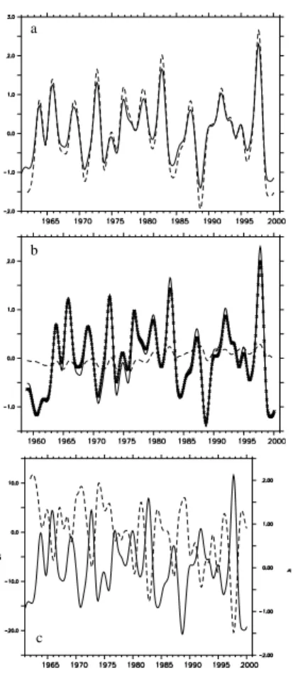
Fig. 3. Temperature variability averaged over the Ni ˜no3 region, interannually filtered; (a) SST from Reference experiment (REF-05, solid line) and COADS observational data (dashed line); (b) SST (solid line) and T80(dashed line) anomalies for REF-05.
OSD
4, 529–569, 2007 A model simulation of Pacific STC variability J. F. L ¨ubbecke et al. Title Page Abstract Introduction Conclusions References Tables Figures ◭ ◮ ◭ ◮ Back CloseFull Screen / Esc
Printer-friendly Version Interactive Discussion
EGU
Fig. 4. Meridional section of the mean zonal velocity (in m/s) at 155◦W; positive values denote eastward velocities; (a) REF-05 (b) REF-025.
OSD
4, 529–569, 2007 A model simulation of Pacific STC variability J. F. L ¨ubbecke et al. Title Page Abstract Introduction Conclusions References Tables Figures ◭ ◮ ◭ ◮ Back CloseFull Screen / Esc
Printer-friendly Version Interactive Discussion
EGU
Fig. 5. Velocity averaged over one year between 50 m and 150 m (in m/s); the colourbar displays the speed while the vector lengths are strongly scaled to a maximum value.
OSD
4, 529–569, 2007 A model simulation of Pacific STC variability J. F. L ¨ubbecke et al. Title Page Abstract Introduction Conclusions References Tables Figures ◭ ◮ ◭ ◮ Back CloseFull Screen / Esc
Printer-friendly Version Interactive Discussion
EGU
Fig. 6. Meridional velocity in a section across 7◦S (off New Guinea) for (a) REF-2, (b) REF-05, (c) REF-025.
OSD
4, 529–569, 2007 A model simulation of Pacific STC variability J. F. L ¨ubbecke et al. Title Page Abstract Introduction Conclusions References Tables Figures ◭ ◮ ◭ ◮ Back CloseFull Screen / Esc
Printer-friendly Version Interactive Discussion EGU a b c
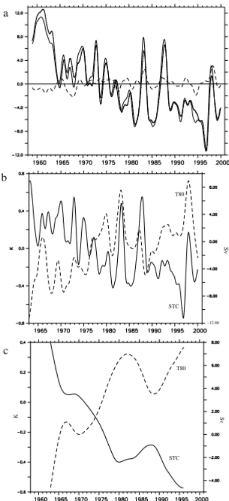
Fig. 7. Temperature variability averaged over the Ni ˜no3 region, interannually filtered; (a) T80 anomalies for REF-05 (solid line) and REF-025 (dashed line); (b) T80 anomalies for REF-05 (solid line), HEAT+SALT (dashed line) and WIND (crossed line) (c) T80anomalies (solid line) and EUC transport anomalies at 155◦W (dashed line), both for REF-05.
OSD
4, 529–569, 2007 A model simulation of Pacific STC variability J. F. L ¨ubbecke et al. Title Page Abstract Introduction Conclusions References Tables Figures ◭ ◮ ◭ ◮ Back CloseFull Screen / Esc
Printer-friendly Version Interactive Discussion
EGU
a
b
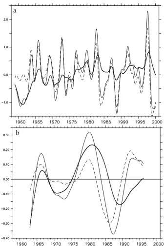
Fig. 8. T80anomalies averaged over the Ni ˜no3 region for REF (solid line), EQ (dashed line) and NO EQ (dotted line); (a) interannually, (b) decadally smoothed.
OSD
4, 529–569, 2007 A model simulation of Pacific STC variability J. F. L ¨ubbecke et al. Title Page Abstract Introduction Conclusions References Tables Figures ◭ ◮ ◭ ◮ Back CloseFull Screen / Esc
Printer-friendly Version Interactive Discussion EGU Sv T80 STC −12.00 K Sv STC T80 a b c
Fig. 9. Anomalies of the STC strength (a) for REF (solid line), EQ (dashed line) and NO EQ (dotted line), interannually smoothed; (b) for NO EQ (solid line) and of Ni ˜no3 T80(dashed line), interannually smoothed; (c) same as (b) but decadally smoothed.
OSD
4, 529–569, 2007 A model simulation of Pacific STC variability J. F. L ¨ubbecke et al. Title Page Abstract Introduction Conclusions References Tables Figures ◭ ◮ ◭ ◮ Back CloseFull Screen / Esc
Printer-friendly Version Interactive Discussion
EGU
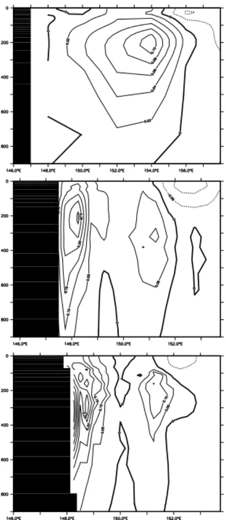
Fig. 10. Standard deviation of v′ ¯T, integrated across the density range of the equatorward layer (σ=22.5 to 26.2 for the southern and σ=22.0 to 26.0 for the northern hemisphere) and decadally smoothed.
OSD
4, 529–569, 2007 A model simulation of Pacific STC variability J. F. L ¨ubbecke et al. Title Page Abstract Introduction Conclusions References Tables Figures ◭ ◮ ◭ ◮ Back CloseFull Screen / Esc
Printer-friendly Version Interactive Discussion
EGU
Sv Sv
Fig. 11. Interannually smoothed net equatorward transport across (a) 6◦S to 10◦S and (b) 6◦N to 10◦N in the STC density range; total transport (black) separated into transport at the western boundary (red) and in the interior basin (green).
OSD
4, 529–569, 2007 A model simulation of Pacific STC variability J. F. L ¨ubbecke et al. Title Page Abstract Introduction Conclusions References Tables Figures ◭ ◮ ◭ ◮ Back CloseFull Screen / Esc
Printer-friendly Version Interactive Discussion
EGU
b a
Fig. 12. Linear trend as a function of latitude for (a) southern and (b) northern cell; total trend (black) separated into trend at the western boundary (red) and in the interior basin (green).