HAL Id: insu-03185196
https://hal-insu.archives-ouvertes.fr/insu-03185196
Submitted on 30 Mar 2021
HAL is a multi-disciplinary open access
archive for the deposit and dissemination of
sci-entific research documents, whether they are
pub-lished or not. The documents may come from
teaching and research institutions in France or
abroad, or from public or private research centers.
L’archive ouverte pluridisciplinaire HAL, est
destinée au dépôt et à la diffusion de documents
scientifiques de niveau recherche, publiés ou non,
émanant des établissements d’enseignement et de
recherche français ou étrangers, des laboratoires
publics ou privés.
Associated Circulation Features
Nada Selami, Geneviève Sèze, Marco Gaetani, Jean-Yves Grandpeix, Cyrille
Flamant, Juan Cuesta, Noureddine Benabadji
To cite this version:
Nada Selami, Geneviève Sèze, Marco Gaetani, Jean-Yves Grandpeix, Cyrille Flamant, et al.. Cloud
Cover over the Sahara during the Summer and Associated Circulation Features. Atmosphere, MDPI
2021, 12 (4), pp.428. �10.3390/atmos12040428�. �insu-03185196�
Article
Cloud Cover over the Sahara during the Summer
and Associated Circulation Features
Nada Selami 1, Geneviève Sèze 2,*, Marco Gaetani 3,4, Jean‐Yves Grandpeix 2, Cyrille Flamant 4, Juan Cuesta 5 and Noureddine Benabadji 1 1 LAAR, Genie Physical Department, Faculty of Physics, University of Science and Technology Mohamed Boudiaf, Oran BP 1505, Algeria; nada.selami@univ‐usto.dz (N.S.); noureddine.benabadji@univ‐usto.dz (N.B.) 2 LMD/IPSL, Sorbonne Universités, CNRS, EP, ENS, F 75252 Paris CEDEX 05, France; jean‐[email protected] 3 Classe di Scienze Tecnologie e Società, Scuola Universitaria Superiore IUSS, 27100 Pavia, Italy; [email protected] 4 LATMOS/IPSL, Sorbonne Universités, UVSQ, CNRS, F 75252 Paris CEDEX 05, France; [email protected] 5 LISA/IPSL, UMR 7583 CNRS, Université Paris Est Créteil, Université de Paris, 94010 Créteil CEDEX, France; [email protected] * Correspondence: [email protected]
Abstract: Over the Sahara in summer, the activity of the Saharan thermal low pressure system
(SHL), which is linked to the West‐African monsoon dynamics and the mid‐latitude circulation, is modulated by dust concentration and water‐vapor transport. In this context, the role of clouds over western Sahara remains under‐investigated. Using Meteosat‐Second‐Generation geostation‐ ary satellite data, for the first time the variability of cloud occurrence over Sahara by type in sum‐ mer, at diurnal, daily and intra‐seasonal time scales for the 2008–2014 period is documented. Us‐ ing European Center for Medium‐range Weather Forecasting (ECMWF) Reanalysis (ERA) Interim (ERAI) reanalysis, cloud cover occurrences are characterized in terms of regional circulation pat‐ terns and moisture balance. We show that, over West‐Sahara and Hoggar, mid‐top clouds are the most frequent cloud‐type in summer. Their summit reaches between 500 hPa and 400 hPa and lies just above the top of the Saharan Atmospheric Boundary Layer (SABL). During the rest of the year, high‐top clouds are the most frequent. The variations in the spatial distribution of mid‐top cloud occurrence coincide with the seasonal displacement and strengthening of the SHL and, in the mid‐troposphere, of the Saharan anticyclone. Mid‐top clouds occur most frequently when, at large scale, mass and humidity converge in the lower SABL due to heating on an extensive sur‐ face, and diverge in the upper SABL. Their diurnal cycle, with minimal frequency around 10 UTC and maximum in the evening, is consistent with the diurnal development of the Saharan Convec‐ tive‐Boundary‐Layer. The frequency of high cloud increases when anticyclonic circulations at mid‐level and upper‐level retreat to the southeast and upper‐level trough from mid‐latitudes can penetrate more southwards.
Keywords: mid‐level clouds; Saharan boundary layer; heat low; climatology; satellite
observations; moisture convergence 1. Introduction Atmospheric dynamics in the Sahara region is a key element of the climate system, interconnected with the Atlantic to the west, the Mediterranean to the north and the Sa‐ hel and tropical West Africa to the south. In summer, the atmospheric circulation in this region is particularly complex. On the one hand, mass and moisture flows from sur‐ rounding regions modulate the local thermodynamics [1,2]. On the other hand, atmos‐ pheric dynamics in the Sahara impacts climate and synoptic variability at the regional scale as a major component of the West African Monsoon [3–5]. Above northern Africa, Citation: Selami, N.; Sèze, G.; Gaetani, M.; Grandpeix, J.‐Y.; Fla‐ mant, C.; Cuesta, J. Cloud Cover over the Sahara during the Summer and Associated Circulation Features. Atmosphere 2021, 12, 428. https:// doi.org/10.3390/atmos12040428 Academic Editor(s): George Kallos Received: 11 February 2021 Accepted: 22 March 2021 Published: 26 March 2021
Publisher’s Note: MDPI stays neu‐
tral with regard to jurisdictional claims in published maps and insti‐ tutional affiliations.
Copyright: © 2021 by the authors.
Licensee MDPI, Basel, Switzerland. This article is an open access article distributed under the terms and conditions of the Creative Commons Attribution (CC BY) license (http://creativecommons.org/licenses /by/4.0/).
the circulation in the upper troposphere is dominated by the western portion of the Ti‐ betan high, associated with the Indian monsoon deep convection [6]. The main axes of the resulting anticyclonic circulation are the sub‐tropical westerly jet (STWJ), flowing along the North African coast, and the tropical easterly jet (TEJ), located above equatori‐ al Africa [6]. In the mid troposphere, the Sahara is dominated by an anticyclonic circula‐ tion associated with the subsidence of the descending branch of the meridional Hadley circulation, and maintained by the radiative cooling in the upper troposphere [6]. The lower troposphere is dominated by the Saharan heat low (SHL), a near surface thermal low pressure developing over western Sahara in response to the radiative warming of the surface [4]. The cyclonic circulation associated with the thermal low drives the mois‐ ture transport from the subtropical North Atlantic and the Mediterranean across the de‐ sert [2,5].
The Sahara is the world’s largest dust source [7]. In summer in its western part, the Sahara is characterized by the deepest atmospheric boundary layer (the so‐called Sa‐ haran atmospheric boundary layer—SABL) on Earth when the SHL, in its north‐ westward migration, reaches this region [4]. In the SABL, aerosols and water vapor are mixed and processed up to 6–7 km in the troposphere, with clouds often formed on its top [8–11]. The physical mechanisms controlling the complex interactions among aero‐ sols, water vapor and clouds, are still far from being completely understood, casting un‐ certainty on the modeling of the radiative budget and atmospheric dynamics in this re‐ gion [12]. This incompleteness is a crucial limitation for climate modeling and predicta‐ bility at regional and global scale, demanding substantial improvements [13]. Cloud cover distribution especially above the Sahara and the mechanisms leading to its for‐ mation are barely reported in the literature. During the JET2000 campaign [14], Parker et al. [8] identified from aircraft measurements a high level of relative humidity in the up‐ per part of the SAL (Saharan Air Layer) and observed clouds at this level. Then in the framework of AMMA (Analyses multidisciplinaires de la mousson africaine) project [15] and Fennec [16] field campaigns, several papers were published including observations of clouds over the western Sahara. For example, observations of clouds and their diurnal cycle have been described by Cuesta et al. [9], who collected light detection and ranging (lidar) data on the ground at the Tamanrasset weather station in the Hoggar massif (Fig‐ ure 1) during AMMA in 2006. In summer, in the afternoon, simultaneous to the growth of a convective boundary layer, lidar data show the development of clouds at the top of the SABL lasting until evening and even late evening during periods of strong dry con‐ vection. Marsham et al. [17], from measurements over western‐central Sahara at the Bordj Badji Mokhtar Supersite‐1 (Figure 1) during the Fennec experiment in June 2011 show that the cloud cover reaches its maximum between 18 UTC and 21 UTC whilst the SABL top height decreases after 18 UTC but the moistening above increases until 21 UTC. Another finding is that dusty days tend to also be cloudy. Kealy et al. [18] also de‐ scribe cloud located at the top of the SABL and the broken aspect of this cloud cover from airborne lidar and radiometer data collected during the Fennec experiment. Com‐ paring this data set with MET Office retrievals from Meteosat‐Second‐Generation geo‐ stationary satellite data, Kealy et al. [18] suggest the possibility of cloud cover overesti‐ mation due to the fragmentation of this cloud cover associated with the frequent occur‐ rence of dust uplift. Stein et al. [19], Bouniol et al. [20] and Bourgeois et al. [21] analyzing the daily data (around 01.30 and 13.30, equator‐crossing local time) from the space‐borne lidar CALIOP and radar CLOUDSAT over West Africa, show that clouds in summer over western Sahara are placed at the top of the SABL (~500 hPa). These clouds occur more frequently during nighttime than daytime. All these studies are limited however in both space and time coverage and do not allow a complete description of the cloud cov‐ er distribution over the Sahara in summer.
Figure 1. Map of West Africa with relief, July position of sub‐tropical westerly jet (STWJ, blue line)
[22], maximum monthly mean rainfall (dashed black line) [22], northernmost position of monthly mean rainfall > 25 mm (dotted red line) [22], the contours of the West‐Sahara and Hoggar regions (garnet), the Tamanrasset meteorological station (green star) and the supersite‐1 of Bordj Badji Mokhtar during the Fennec experiment (red star). For the altitude, the isolines are given every 200 m from 400 m. Altitude above 1200 m (light purple).
The objectives of this paper are to provide a more complete description of the cloud cover distribution in the region of the central western Sahara and the Hoggar massif, where the SHL builds up in summer, and to characterize the cloud cover occurrence in relationship with circulation patterns and moisture convergence over this region. With this aim in mind, a climatology of cloud type occurrence during boreal summer (June to September, JJAS) from 2008 to 2014 has been built. This is the first quantification of cloud occurrence by type over the Sahara during summer and of its spatial distribution, from diurnal to intra‐seasonal scales. To do that, SAFNWC (Satellite Application Facility for Now‐casting) cloud observations at high temporal and spatial resolution obtained from Meteosat Second Generation (MSG) geostationary satellites are used. Atmospheric variables from the European Center for Medium‐range Weather Forecasting (ECMWF) Reanalysis (ERA) Interim product are used to identify the circulation and moisture con‐ vergence patterns over this region which are linked to different cloud cover types. Anal‐ yses are conducted separately for the central western Sahara (hereafter called the West‐ Sahara) where the SHL is established in July and August [4] and for the mountainous Hoggar area (hereafter referred to as Hoggar) to the east and south of which the SHL is located in June before the monsoon onset [4,9,23]. Their boundaries are shown in Figure 1. To simplify the analysis, the West‐Sahara does not include the coastal region which is subject to a stationary sea breeze front during the day which penetrates the land during the night [24,25].
The paper is organized as follows. Satellite retrievals and reanalysis products are presented in Section 2, along with a description of the cloud type classification method. In Section 3, the main climatological features of cloud cover over West Africa are pre‐ sented followed by a more precise description of the cloud cover occurrence over the West‐Sahara and Hoggar. At the same time, the main elements of the atmospheric circu‐ lation over the Sahara and Sahel are given in summer. In Section 4, cloud cover occur‐ rence is characterized over the West‐Sahara and Hoggar in terms of the regional circula‐ tion patterns and moisture balance. Section 5 first provides a seasonal scenario of large‐ scale conditions and of the development of a deep SABL over the Sahara and mid‐top cloud cover occurrence, and then discusses the main characteristics of the SABL and its diurnal cycle and the possible impact of a change in these characteristics on the occur‐ rence of mid‐top clouds. A summary and conclusion are provided in Section 6.
2. Data
2.1. Spinning Enhanced Visible and Infrared Imager (SEVIRI) Data and the Satellite Application Facility for Now‐Casting (SAFNWC) Cloud Algorithm
The SEVIRI (Spinning Enhanced Visible and Infrared Imager), onboard the geosta‐
tionary satellite MSG (METEOSAT second Generation,
http://www.eumetsat.int/website/home/Satellites/index.htm (accessed on 23 March 2021)), is a visible and infrared multi‐channel imager which observes the Earth’s atmos‐ phere and surface at 13 different wavelengths: 3 visible channels, 2 near‐infrared chan‐ nels and 8 infrared channels. A very important feature of SEVIRI is its continuous imag‐ ing of the Earth, with a baseline repeat cycle of 15 min. The imaging sampling distance is 3 km × 3 km at nadir for standard channels, and down to 1 km for the high‐resolution visible (HRV) channel.
Cloud types and cloud top pressure used in our studies are produced with the SAFNWC software (www.nwcsaf.org (accessed on 23 March 2021)) applied to SEVIRI data. The algorithm used in this software was developed within the framework of the Eumetsat Satellite Application Facility in support for Now Casting and very short range forecasting (NWC SAF). It is described in the Algorithm Theoretical Basis Document written by Derrien and Legleau [26]. Here is a summary of the main features of this al‐ gorithm which is applied to each pixel and performed in three steps: (1) cloud detection, (2) cloud type classification, (3) cloud to pressure determination. For the first step, one can find more concise information on the algorithm in Derrien and Le Gleau [27,28].
In step 1, to separate clear pixels from cloudy pixels, a series of threshold tests are applied sequentially [26–28]: tests on window channel brightness temperatures (BT at 10.8 μm) and bi‐directional reflectance (at 0.6 μm or 0.8 μm) but also differences of brightness temperature between two wavelengths (chosen among 10.8 μm, 12 μm, 3.9 μm, 8.7 μm), on spatial and temporal variability of BT at 10.8 μm and spatial variability of bi‐directional reflectance. The set of thresholds to be applied depends mainly on the illumination conditions (nighttime, twilight, daytime). With the exception of the spatial and temporal variability tests, the values of the thresholds themselves depend on ancil‐ lary data such as the illumination, the viewing geometry, the geographical location and numerical weather prediction model data giving the total column water vapor content and 925 hPa air temperature, monthly SST (Sea Surface Temperature) climatology, and over land reflectance climatology. These values are computed from simulated clear sky BT and bi‐directional reflectance simulated by the RTTOV (Radiative Transfer for TOVS) radiative transfer model [29] for thermal bands and the 5S radiative transfer model for the solar spectrum [30] for the atmospheric and surface conditions given by the ancillary data set. In step 2, the method for assigning a cloud type to cloud pixels is based on the same approach as in step 1 (i.e., a set of threshold test on BT, differences on BT, and spatial variability of BT and reflectance). To the ancillary data set used in step 1 is added a coarse description of the temperature and humidity profiles using numerical weather prediction model profiles. This classification process, at the end of which 10 classes of clouds are defined, makes it possible to differentiate thick cloud from thin cloud or par‐ tial cloud cover. This cloud pixel partitioning is used in step three to choose the cloud height algorithm applied to each cloudy pixel.
In step 3, the cloud top height (CTH) for opaque clouds (clouds with IR emissivity close to 1) is retrieved from the common IR (10.8 μm) brightness temperature by consid‐ ering them as black bodies. For low/mid‐level clouds, tests are applied so as to place the CTH below the altitude of the temperature inversion where one exists. For thin clouds, a correction for semi‐transparency is applied using two infrared (IR) channels, as in Schmetz et al. [31] and Menzel et al. [32]. For partial cloud cover, no cloud top pressure is given. For partial cloud class pixels, which correspond to very thin clouds, small cu‐
mulus, broken cloud cover [26,33], cloud edges, cloud top pressure retrieval is not pos‐ sible [26].
The main limitations of the SAFNWC cloud algorithms are given in Derrien and Le Gleau [26] and an evaluations of the cloud products against CALIOP (Cloud‐Aerosol Lidar with Orthogonal Polarization) space‐borne lidar and CLOUDSAT space‐borne ra‐ dar data is given in Kerdraon and Le Gleau [34] (see also Seze et al. [33], Hamann et al. [35]). 2.2. Cloud Top Pressure and Cloud‐Type Classification over Sahara Initially, the eleven SAFNWC cloud types (clear sky, very low‐top clouds, low‐top clouds, mid‐top clouds, thick high‐top clouds, both thick and very high high‐top clouds, thin semi‐transparent clouds (cirrus), cirrus, thick cirrus, cirrus above another cloud lay‐ er, partial cloud cover), were grouped together to establish a classification according to the three main cloud types, low‐top clouds, mid‐top clouds and high‐top clouds. How‐ ever, the analysis of the repartition of cloud top pressure for each classes inside the whole cloud top pressure over Sahara show that part of thin cirrus could be in fact mid‐ top clouds. For this reason, it was decided to construct the classification into low‐top clouds, mid‐top clouds and high‐top clouds using the SAFNWC cloud top product and two thresholds dividing the troposphere into three parts: lower troposphere, middle‐ troposphere and upper troposphere. 350 hPa and 500 hPa were retained as thresholds (see Appendix A). For partial cloud cover for which no cloud top pressure is available, to assign a lev‐ el to these SEVIRI partially cloudy pixels, the same approach as in Dommo et al. [36] is used: each pixel of the partial coverage class is reclassified as high‐top, mid‐top or low‐ top cloud depending on the distribution of these three cloud types in the vicinity of the pixel (see Appendix B).
Both the choice of the cloud top pressure thresholds and the results of the re‐ classification process of the SEVIRI partial cloud cover have been evaluated in a compar‐ ison with the CALIOP lidar data carried out using statistics and pixel‐by‐pixel compari‐ sons (see Appendix C). 2.3. European Center for Medium‐Range Weather Forecasting (ECMWF) Reanalysis (ERA) In‐ terim Data Cloud cover occurrence is characterized in terms of large scale circulation patterns and moisture budget in the region by using atmospheric variables extracted from the
ERA‐Interim reanalysis (ERAI) dataset ([37],
https://www.ecmwf.int/en/forecasts/datasets/reanalysis‐datasets/era‐interim (accessed on 23 March 2021)). For the 2008–2014 period, JJAS water vapor path, horizontal and vertical winds, temperature, specific humidity and geopotential height 6‐hourly data, at 0.75° latitude‐longitude resolution (i.e., 80 km at the equator), on 37 vertical levels, in the domain 25° W–35° E and 0° N–45° N, are used. The SHL location is defined following Lavaysse et al. [4]. At each time step, the cu‐ mulative distribution of potential temperature at 850 hPa is computed for the grid points within the 13° W–15° E and 15° N–35° N domain. The SHL location is defined as the area where the potential temperature exceeds the 97th percentile of the spatial distribution. In the following this potential temperature value will be called threshold. A map of the oc‐ currence frequency of the SHL is then constructed for the entire period. In the frequency map, the area within the 15% isoline is chosen to represent the average location of the SHL. The same method is applied to the geopotential height at 600 hPa, to characterize the Saharan anticyclone (SAC), to the geopotential height at 100 hPa and 200 hPa, to characterize the Tibetan anticyclone, and to the geopotential height at 900 hPa, to charac‐ terize the Azores anticyclone. The research domain, the frequency in the cumulative po‐ tential temperature or geopotential height distribution to select a threshold at each time step and the value of the final isoline in the frequency map to define the retained area
are summarized in Table S1. The SHL and the SAC are determined at 18 UTC and 12 UTC, respectively, the times of their maximum intensity.
The latitude of the inter‐tropical discontinuity (ITD) which separates the near‐ surface Saharan air from the cooler, moist monsoonal air [38,39,40] is defined here by an isodrosotherm in the 2 m dew point temperature field. Dew point temperature fields at 06 UTC and the isodrotherm 15 °C values [41,22] are used to take into account the northward movement of the monsoonal nocturnal flow [38,40]. However, caution should be exercised in interpreting the daily variations in the ITD. Moisture fluxes at the surface are not only related to the northward progression of the monsoon flow but also to sporadic strong northward rises in moisture fluxes carried by cold pools [42–45]. Moreover, these cold pools generated by deep convection systems which develop over the Sahel are not simulated properly in the ERAI product due to the convection parame‐ terization scheme used [46,47]. In order to determine the levels at which water vapor is transported over the West‐ Sahara and Hoggar regions, the horizontal convergence of water vapor in each layer, av‐ eraged over the domain for each 6‐h time step, is calculated. If delta‐p is the layer thick‐ ness, gamma the domain contour, d‐gamma the line element of gamma, and n the in‐ ward normal to the contour, then the rate at which water vapor enters the domain in that layer reads, at each time‐step:
𝐶
𝑑𝑒𝑙𝑡𝑎
𝑔
𝑞 ∗ 𝑉. 𝑛 ∗ 𝑑
(1)where q and V are the specific humidity and the horizontal wind velocity at the contour point and g the gravitational acceleration. The average convergence of water vapor in the domain of area S and over a period is <C>/S, where <C> is the time average of C. First, the four daily C values were averaged to calculate the daily average water vapor convergence. For a longer period or for a selection of days, the average water vapor con‐ vergence is obtained by averaging the daily values.
The sum of the water vapor convergence should be equal to dPW + E − P, where dPW is the change of the water vapor path between the beginning and the end of the pe‐ riod, P is the average precipitation and E the average evaporation over the surface of the domain. In the present case E – P is very small so that the sum of the incoming fluxes should be equal to dPW, which is in itself small compared to the convergences. Howev‐ er, for the West‐Sahara and Hoggar, the sums for the various months turn out to range between 0.22 and 0.87 kg/m2/d for the West‐Sahara and between 0.28 and 0.48 kg/m2/d
for Hoggar. These values are consistent with Meynadier et al. [48] who find a residual convergence ranging from 1.08 to 1.42 kg/m2/d (see their Table A1) for three domains of West Africa located south of 20° N; the larger values of the residuals of Meynadier et al. [48] may stem from the greater humidity in less dry locations. More frequent cold pools and the greater amount of moisture carried by these cold pools can contribute to these larger residuals. One may expect the positive water budget residual to increase with the intensity of the water cycle in the troposphere. It so happens that the positive water budget residual is approximately proportional to the absolute value of the convergence in the [surface, 850 hPa] layer. For each time period in which the low‐level convergence is always of the same sign, this leads to residuals in the order of 10% of the absolute value of the mean convergence. For periods during which the low‐level convergence changes sign, the re‐ siduals may become proportionally greater. These residuals provide uncertainty in the analysis of levels at which water enters the domain. However, these residuals will not harm the analysis especially in a day to day analysis.
3. Cloud Cover and Cloud Cover Type Occurrence Observed with SEVIRI
In this section, the general features of the summer (JJAS) cloud cover occurrence frequencies (COF) are first presented, for total cloud cover, high‐top clouds, mid‐top clouds and low‐top clouds, over a region including Tropical North Africa, the Sahara, subtropical Northeast Atlantic and the Mediterranean. COF is defined in each SEVIRI pixel as the fraction of cloudy time steps over the total number of 15′ time steps over the 2008 to 2014 period. The main features of the atmospheric circulation, including the northward progression of lower troposphere humidity, the SHL and the SAC positions are also shown. A more detailed study of cloud cover occurrence over West‐Sahara and Hoggar is then presented. 3.1. General Features of Cloud Cover Occurrence over West Africa 3.1.1. Total and High‐Top Cloud Cover Figure 2a,b show monthly average maps of total COF and high‐top COF. Figure 2b also gives the regions where maxima of geopotential height at 200 hPa and 100 hPa are the most frequently located (indicative of the Tibetan anti cyclone position; see Section 2 for the definition of these regions) and the boundary between the easterly and westerly winds at 200 hPa (the zero isoline of 200 hPa zonal wind). In Figure 2b, the northern boundary of the high‐top cloud cover due to the ITCZ convective activity approaches 18° N during the pre‐onset period in June and reaches 20° N during the monsoon peak in August [49]. This limit is close to the northern end of the precipitation belt (Figure 1) (Lélé et al. [50]). Linked to the ITCZ move, in the upper troposphere and mid‐ troposphere the easterly wind regime move also north (see the boundary between west‐ erly and easterly wind in Figure 2b). In September, east of 10 W, the northern limit of the high‐top cloud cover returns to its June position, but west of 10 W, this limit remains close to 20° N. This may be related to the African Easterly Wave (AEW) regime, which peaks in September along the west coast of North Africa [51].
JUNE JULY AUGUST SEPTEMBER (a) (b) Figure 2. (a) Total cloud cover occurrence frequencies (COF, shadings), together with 650 m and 1000 m topography iso‐ lines (brown dashed contours). (b) High‐top COF (shadings), zero isoline of the zonal wind at 200 hPa (black), bounda‐ ries of the most frequent regions for the maximum of geopotential height at 200 hPa and 100 hPa (pink and blue con‐ tours, respectively). Over the eastern Sahara where subsidence induced by the Tibetan high in the upper troposphere, is the strongest, clear sky is very frequent (large number of COF <5% in Figure 2a—gray regions). Over western Sahara and Hoggar this frequency is not so large (COF >10%). From June to July, while the Tibetan high (region of maximum of geopoten‐ tial height at 200 hPa and 100 hpa in Figure 2b) migrates northwestward and subsidence underneath reinforces [52], the clear sky frequency rises over Eastern Sahara but also over the eastern Hoggar massif. The northward shift of the anticyclone, contributes to the STWJ (Figure 1) moving northward and accentuates its tilt towards the northeast over eastern and central Mediterranean. In July, clear sky also predominates over the central and eastern Mediterranean (COF <10% in Figures 2a). In August and September, over the central and eastern Mediterranean and the central and eastern Sahara, as the Tibetan anticyclone gradually retreats to the southeast, the frequency of clear skies di‐ minishes. In Figure 2b, from June to July, the upper cloud cover, relative to total cloud cover, reduces not only in eastern Sahara, but also in western Sahara and the eastern Atlantic. Over the eastern Atlantic, as the descending branch of the Hadley cell pushes the mid‐ latitude flow northward, in the upper troposphere, clear sky frequencies above 95% be‐ come frequent (COF < 5% in Figure 2a). Over western Sahara, which is located between the two subsidence maxima related to the descending branch of the Hadley cell and to the Tibetan anticyclonic circulation, the frequency of high cloud does not reach the min‐ imum values observed over eastern Sahara and the eastern Atlantic. In August, the high‐top COF increases again over the East Atlantic and over the western Sahara. The STWJ begins to migrate southward and with the relaxation of the high pressure belt mid‐latitude lows can penetrate farther south making the environment favorable for possible outbreaks of tropical moist air into the subtropical mid and high troposphere and occurrence of high clouds in these regions [53–55].
3.1.2. Mid‐Top Cloud Cover
The monthly mean of mid‐top cloud COF is given in Figure 3. In this figure is also given the regions where maxima of the SAC (geopotential at 600 hPa) at 12 UTC and where the SHL at 18 UTC are the most frequently located.
JUNE JULY AUGUST SEPTEMBER
Figure 3. Mid‐top COF (shadings), boundaries of the most frequent region for the Saharan anticyclone (SAC, pink contour) and most frequent region for the Saharan heat low (SHL, red contour).
Over the Sahara, west of 10° E, in agreement with the previous studies on cloud cover over this region, Figure 3 shows the occurrence of clouds capped at mid‐level. Compared however to these studies which described the meridional evolution of cloud cover profiles in a 10° W–10° E transect or with airplane or point measure‐ ments, Figure 3 shows that mid‐top COF is not uniformly distributed over the re‐ gion. For example, over the Hoggar the cloud cover can reach 40% in agreement with the cloud cover observed from synoptic surface observations at the Tamanras‐ set weather station (Figure 1) [9]. But the COF is below 20% between the Hoggar and the Atlas. Figure 3 shows also that the location of the maximum of COF differs from one month to the other. In June, the mid‐top cloud cover is mostly concentrat‐ ed over the Hoggar massif and over the Addrar massif to the South‐West. During this period, the SHL (region of maximum potential temperature at 850 hPa in Figure 3) is preferentially located south of the Hoggar. After the monsoon onset in July, the SHL strengthens, moves northwestward [4,49] and reaches the foothills of the Atlas massif in August. The center of the Saharan anticyclone (region of maximum poten‐ tial temperature at 850 hPa in Figure 3) follows the SHL trajectory. From July, mid‐ top cloud cover occurs over the West‐Sahara and the Atlas massif. In September both the SHL and the Saharan anticyclone move to the southeast. The mid‐top cloud cover over the Atlas range decreases, replaced by a large amount of high‐top cloud cover. However, mid‐top cloud is the more frequent cloud type over the West‐Sahara and Hoggar (Figure 3).
3.1.3. Low‐Top Cloud Cover
Figure 4 shows the monthly mean of low‐top cloud COF with superimposed the horizontal wind at 925 hPa, the ITD (the iso‐drotherm 15 °C in the 2 m dew point temperature field) and the regions where maxima of geopotential at 900 hPa is located (Azores Anticyclone).
JUNE JULY AUGUST SEPTEMBER
Figure 4. Low‐top COF (shadings), inter‐tropical discontinuity (ITD, black line), boundaries of the most frequent region
for the geopotential at 900 hPa (green line), horizontal wind at 925 hPa (vectors).
Over southern West Africa, on the south part of the ITCZ (Figure 1), the low clouds are frequent in July and August, when the high‐top clouds, which obscured the low cloud cover in June in the SEVIRI data, move northward. This illustrates the penetration of the monsoonal moisture flow [19,20,50,56] from the ocean to the mainland, which feeds the deep convection within the ITCZ. Holle et al. [57] and Stein et al. [19], using cloud profiles obtained from combined lidar and radar data, determined that the fre‐ quency of low clouds was maximum just south of 7°–8° N. Here, with visible (VIS) and IR SEVIRI data, such behavior is not observable. From the equator northward, the fre‐ quency of low‐top COF decreases (Figure 4) whilst the high‐top COF increases (Figure 2b) indicating that low clouds occur more and more frequently under high‐clouds when going northward until 7°–8° N. On the other hand, Van der Linden et al. [58] show that SAFNWC low‐top COF close to the Guinean coast is underestimated during nighttime due to a poor separation with clear sky. On the northern boundary of the high cloud cover at 15° N (see Figure 2b) the frequency of low‐top cloud (Figure 4) is low. This is in agreement with the observations of Parker et al. [8] during the JET2000 experience, showing the small occurrence of low‐top cloud just north of the AEJ (African Easterly Jet). These observations are confirmed by the results of CALIOP/CLOUDSAT analysis of Stein et al. [19]. But the low‐top COFs observed in Figure 4, although low, are higher than those given by the CALIOP climatology. Over the Sahara, the SEVIRI‐derived low clouds are in fact most often detected as broken edges of mid‐top clouds or as clear air in the CALIOP data set (seeAppendix C ). It can be noted that the northward progression of the ITD from June to August, as well as its withdrawal in September, coincides well with that of the high‐top clouds (Figure 2b) over the same period. 3.2. Intra‐Seasonal Evolution of Cloud Cover over the Hoggar and the West‐Sahara To specify the characteristics of the cloud cover over the Sahara and their evolution during the summer, the emphasis is on the two regions where the occurrence of mid‐ high clouds is the most frequent, but which do not show the same intra‐seasonal evolu‐ tion: the massif of the Hoggar and the region of the West‐Sahara (Figure 1). For these two regions the total, mid‐top and high‐top COF are calculated at each 15′ time step and are then averaged throughout the day. T DCOF, H DCOF and M DCOF are the daily to‐ tal, high‐top and mid‐top cloud occurrence frequencies, respectively. The low‐top cloud class is renamed as very‐partial cloud cover class (see Appendix C) and its occurrence frequency is calculated for both regions. VP DCOF is the daily very‐partial cloud COF. Firstly, monthly average statistics, including cloud top pressure distribution and cloud frequencies diurnal cycle are analyzed. Then the evolution of the daily cloud frequency of high‐top clouds and mid‐top clouds (H DCOF and M DCOF) during the season and the peculiarities of these frequencies compared to the rest of the year are discussed.
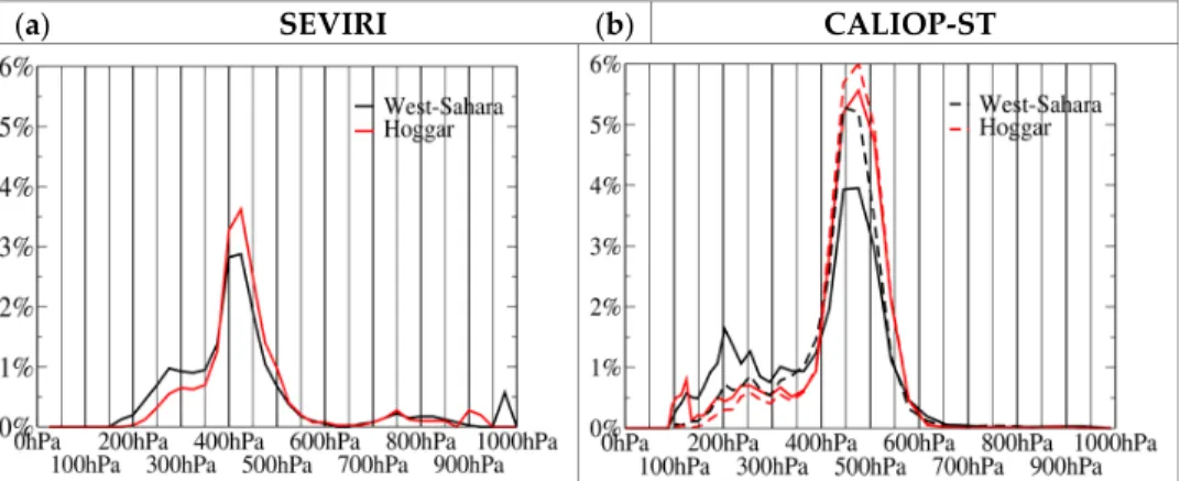
3.2.1. Monthly Mean Statistics Figure 5a shows the distribution of cloud top pressure over western Sahara and the Hoggar. In this distribution, the peak at 400 hPa indicates that the cloud cover is prefer‐ ably at this altitude which is close to but above the SABL top in agreement with observa‐ tions from lidar data (see Appendix C and [9,10,18–21]). In July, when the frequency of high‐top clouds is low (Figure 2b), the distributions are reduced almost to a single peak, whilst in June and September over the West‐Sahara, a secondary peak appears at 275 hPa.
JUNE JULY AUGUST SEPTEMBER
(a)
(b)
(c)
high‐top clouds mid‐top clouds very partial cloud cover
Figure 5. (a) Cloud top pressure occurrence frequency distributions for West‐Sahara (black line) and Hoggar (red line).
(b) for West‐Sahara and (c) Hoggar, the diurnal evolution of the COF at 15′ time step averaged over one hour.
To construct Figure 5a, pixels belonging to the very‐partial cloud cover class were retained when a pressure level was available (i.e., pixels classified as low cloud in the SAFNWC classification prior to the partial cloud cover pixel reclassification process). This shows the very small contribution of these “false” low clouds if CALIOP is taken as reference (see Appendix C). In Figure 5b for the West‐Sahara and Figure 5c for the Hoggar, the diurnal cycle of the occurrence frequencies of mid‐top and high‐top cloud cover and very partial cloud cover is given. The diurnal cycle of mid‐top cloud COF is characterized by a minimum during the morning and an increase during the afternoon to reach its maximum in the evening. It clearly agrees with the diurnal cycle of cloud cover observed with a ground‐ based lidar over the Hoggar in summer 2006 [9] and over the site of Bordj Badji Mokhtar (21.38 N, 0.92 E) (Figure 1) during the Fennec experiment in June 2011 [21]. In the clima‐ tology of cumulus diurnal cycle built by Eastman et al. [59] using synoptic surface ob‐ servations from stations located between the Hoggar and the Atlas (Figure 1), cumulus occurrence peaks in the late afternoon (between 16 UTC and 21 UTC). Using the same synoptic surface observations climatology and for the 4 stations included in the Hoggar and West Sahara regions (2 in the Hoggar and 2 in the West‐Sahara), it is found that the two most frequent cloud types are cumulus and alto‐cumulus. The cumulus cloud oc‐ currence peaks between 17 UTC and 18 UTC but that alto‐cumulus occurrence peaks be‐ tween 23 UTC and 02 UTC.
In the SEVIRI data, the very‐partial cloud cover COF reaches a maximum in the af‐ ternoon when cloud must begin to form at the top of the boundary layer. This very par‐ tial cloud cover could correspond to what observers from the ground call cumulus clouds in this very arid region. The strong discontinuity in very partial cloud cover fre‐ quency at twilight above the West‐Sahara is an artefact of the method. Over the Hoggar where the orography enhance convection process, in surface observations, cumulus clouds are the most frequent cloud type, while over West‐Sahara, alto‐cumulus clouds are more frequent. This is consistent with the decrease in mid‐top cloud cover in the ear‐ ly hours of the night, whereas over West‐Sahara, mid‐top cloud cover persists until late into the night (04 UTC). It is also noted that the largest amplitudes in diurnal variations of mid‐top clouds occurrence are over Hoggar.
3.2.2. Intra‐Seasonal and Seasonal Evolution of Daily Cloud Frequencies
Figure 6a–c show the distributions of high‐top DCOF, mid‐top DCOF and VP DCOF built over 15 day periods for West‐Sahara (left) and Hoggar (right)s. To highlight the particu‐ larities of the cloud cover during the JJAS period compared to the period from October to May, the whole annual cycle is given. The same pressure thresholds to differentiate between low‐top, mid‐top and high‐top clouds were used for the October to May period than those used for the JJAS period even though the frequency of occurrence of a cloud type may be slightly under‐ or over‐estimated (see Appendix C). West‐Sahara Hoggar (a) (b) (c) Figure 6. (a) annual cycle of the distributions of high‐top daily cloud cover occurrence frequency (DCOF) distributions built over 15 day periods for West‐Sahara (left) and Hoggar (right). (b,c) same as (a) but for mid‐top DCOF and daily very‐partial cloud cover occurrence frequency (VP DCOF), respectively. Each 15 day distribution has been partitioned in three parts, using the 5% percentile, 15% percentile, 85% percentile and 95% percentile. The brown areas span the part of the distribution within the 15th and 85th percentiles, the gray areas span the part of the distribution within the 5th and 95th percentiles. Dashed black lines indicate the 50th percentile, solid black lines indicate the 70th percentile, crosses in‐ dicate the maximum values. From June to September, mid‐top cloud cover is the most frequent cloud type (Fig‐ ure 6b; Table S2. During this period, more than 30% of the time the daily occurrence fre‐ quency of mid‐top clouds (M DCOF) is above 10%. In Figures 6b, in mid‐May, M DCOF increases to dominate the cloud cover up to mid‐October, whilst H DCOF decreases over
the Hoggar and the West‐Sahara, reaching its yearly minimum in mid‐July (Figure 6a). In summer, VP DCOF almost never exceeds 10%.
In the following, each day is classified from its frequency values T DCOF, M DCOF and H DCOF. Based on this classification a more in‐depth analysis of the intra‐seasonal evolution of the mid‐top and high‐top cloud cover occurrence during summer is per‐ formed. To build this classification, a 10% threshold to select mid‐top cloud days and high‐top cloud days is used. A mid‐top day is a day with tM DCOF above 10% and H DCOF below 10%. A high‐top day is a day with H DCOF above 10%. Adding a con‐ straint on M DCOF, a high‐top day can be either a high‐top‐alone day when M DCOF is below 10% or a high‐top‐plus‐mid‐top day when M DCOF is above 10%. Clear days are days where M DCOF is below 8%, H DCOF is below 8% and T DCOF (the total cloud cover occurrence frequency) is below 18%. The constraint on T DCOF value is added, in order to exclude days with a large fraction of very partial cloud cover pixels. From these criteria, 90% of the days are classified. The 10% remaining will be not taken into account in the following analysis. Figure 7 gives the evolution by 15‐day period of the frequency of each of the four classes from January to December for the West‐Sahara and the Hog‐ gar. In Figure 8, to better illustrate the east to west progression of the mid‐top day and high‐top day occurrence frequencies during the JJAS period, the West Sahara is divided into three sub‐regions and the Hoggar into two sub regions using thresholds in longi‐ tude (8° W and 3° W for West‐Sahara and 9° E for Hoggar). West Sahara (a) Hoggar (b) Figure 7. (a) Frequencies of mid‐top days, high‐top days and clear days for West‐Sahara. (b) Fre‐ quencies of mid‐top days, high‐top days and clear days for Hoggar. For the 2008–2014 period and 15‐day periods. In Figure 8, at the beginning of June in the eastern Hoggar, the frequency of mid‐ top days reaches its seasonal maximum. During the second half of June while this fre‐ quency decreases in the eastern Hoggar, it increases over the western Hoggar and over the eastern West‐Sahara. In July, the maximum of mid‐top day frequency is located over the central West‐Sahara. During the last half of July over the western West‐Sahara the mid‐top day frequency increases and reaches its maximum value. In August, the fre‐ quencies decrease first over the central West‐Sahara, then over the western West‐Sahara, whilst increasing again over the Hoggar and reaching a peak in late August over the western Hoggar. The frequency of high‐top days is at its highest on the Hoggar and in the eastern West‐Sahara at the beginning of June. Then, after a very sharp decrease in Ju‐
ly, it increases again in August, peaking in late August over the West‐Sahara and then over the western and central West‐Sahara in September (Figure 8). Throughout the sea‐ son, high‐top days are high‐top plus mid‐top days above the relief of the Hoggar (Figure 7b). In the first half of June, their frequency is as large as that of mid‐top days. Over the West‐Sahara, it is only in the second part of the summer that high‐top days are the most frequently days with both high‐top clouds and mid‐top clouds (Figure 7a). (a)
Western W‐Sahara Central W‐Sahara Eastern W‐
Sahara Western Hoggar Eastern Hoggar
(b ) Figure 8. (a) Maps of the division of West Sahara in 3 sub‐regions and of the Hoggar in 2 sub‐ regions. (b) Frequencies of mid‐top days (solid line) and high‐top days (dashed‐dotted line) for each sub‐region and for 15 day periods. Average frequency during JJAS (June to September) over the sub‐region (bleu line) and mean of the average frequency of the 2 Hoggar and 3 Western Saha‐ ra sub‐regions (turquoise line). 4. Mid‐Top Cloud and Regional Atmospheric Conditions The goal of this section is to characterize the strength and position of the SAC and SHL, the ITD position, the importance of the SABL and the fluxes of air mass and water vapor entering the West‐Sahara and Hoggar when mid‐top days occur and to compare these characteristics to those observed during cloud‐free days. For each of these two re‐ gions, the geopotential height at 600 hPa (Z600), the potential temperature (T850) and the total column water vapor (TCWV) are also analysed. Moreover moisture variables (moisture and mass fluxes, ITD position, TCWV) are analyzed for high‐top days. In the figures showing sample mean values, the error bars, when present, give the statistical uncertainty of the mean value, that is, the standard deviation of each sample divided by the square root of the number of days in the sample. 4.1. Intra‐Seasonal Behavior of the Saharan Anticyclone (SAC), the Saharan Heat Low (SHL) and the Inter‐Tropical Discontinuity (ITD) with Mid‐Top Cloud Figure 9a,b show the evolution of the mean location of the daily barycenters of the SAC and SHL (see Section 2.3) during the JJAS period split into 15‐day periods for mid‐ top days and clear days. Figure 10a,b provide information on daily variability in longi‐ tude around these mean values: the frequency of daily barycenter longitude (i) east of 3° E (ii) between 3° E and 3° W and (iii) west of 3° W. In Figure 11a,b, the strength (mean value in the region of the maximum values) of the SAC and the strength of the SHL are given as well as the Z600 and T850 values. Figure 11c,d give, respectively, the ITD aver‐ age latitude at 6 UTC south of each of the regions (12.75° W–0° W for the West‐Sahara and 0° W–12.75° E for the Hoggar) and the mean TCWV value at 18 UTC.
West‐Sahara Hoggar (a) SAC (b) SHL Figure 9. (a) Position of the SAC in a latitude‐longitude coordinate frame for mid‐top (black) and clear days (red). (b) Position of the SHL for mid‐top (black) and clear days (red). Average over 15 day periods of the daily positions. Numbers indicate the month (i) which fall in the first fraction (i.1) or second fraction (i.2). Information given for West‐Sahara (left column) and for Hoggar (right column). The dotted blue lines give a rough representation of Hoggar and West‐Sahara bounda‐ ries. West‐Sahara Hoggar (a) SAC (b) SHL
Figure 10. (a) For the SAC barycenter for mid‐top days, occurrence frequency of the barycenter
longitude on the west of 3° W (yellow contour), between 3° W and 3° E (cyan contour) and on the east of 3° E (brown contour). (b) For the SHL barycenter and for mid‐top days, occurrence fre‐ quency of the barycenter longitude on the west of 3° W (yellow contour), between 3° W and 3° E (cyan contour) and on the east of 3° E (brown contour). The fill part of the bar gives the difference
in frequency between mid‐top days and clear days. Data estimated over 15 days periods. Infor‐ mation is given for West‐Sahara (left column) and for Hoggar (right column).
4.1.1. SHL and SAC Positions and Intensity
For both regions in Figure 9, the SHL barycenter and the SAC barycenter during mid‐top days and during clear days migrate to the north‐west as was observed on the monthly mean maps (Figure 3) and then retreats to the south‐east at the end of August. Figure 9 shows also that the SAC barycenter moves further north and reaches the Atlas foothills, while the SHL barycenter remains south of 27° N at the limit of West‐Sahara (Figure 9b). In both cases (mid‐top days and clear days), the SAC intensity value in‐ creases until the end of July and then decreases (Figure 11a). The SHL also intensify until the end of July and then decreases.
Besides these mean behaviors, over the Hoggar, the SHL is more on the East during mid‐top days than clear days and closer from the Hoggar. The SHL intensity does not show clear differences while the SHL shows higher values of the regional average T850 during mid‐top days (Figure 11b). But, this increase in T850 during mid‐top days is lim‐ ited to eastern Hoggar (see Figure S1). For the SAC, when it is centered east of 3° E, mid‐ top days are more frequent but no systematic behaviour is observed in the relative posi‐ tion of the SAC during mid‐top days compared to clear days in Figures 9a and 10a. The SAC intensity during mid‐top days is slightly weaker than during clear days, although the averaged value Z600 is stronger, indicating a regional cooling in the upper‐mid troposphere characterizing mid‐top days (Figure 11a).
Over West‐Sahara during mid‐top days, the SAC is stronger than during clear days and this difference is even more marked for the average value over the region Z600, in‐ dicating upper‐mid troposphere cooling (Figure 11a). During mid‐top days, the bary‐ center of the SAC is more to the East (Figures 9a and 10a). For the SHL, a position be‐ tween 3° E and 3° W is more frequently associated with mid‐top days than clear days, except in June, when the SHL begins to migrate towards the West‐Sahara. Neither the intensity of the SHL nor the T850 show clear differences between clear and mid‐top days with the exception of the western West‐Sahara (See Figure S1).
Dalu et al. [60] showed that the strength and position of SAC are tightly related to the SHL dynamics. The SHL drives a Walker‐like subsiding to the west, which in turn reinforces the SAC. Chen [6] showed that the SAC dynamics is also influenced by the subsidence associated with the Tibetan anticyclone in the upper troposphere. A more western position of the SAC (SHL) over West‐Sahara (Hoggar) during clear days than mid‐top days, while the same pattern is not observed for the SHL (SAC), could reflect changes in on the relative contributions of the SHL and the Tibetan anti‐cyclone on the SAC position. However, to disentangle these different contributions only on the basis of reanalysis data is not possible and beyond the scope of the paper.
4.1.2. The Inter‐Tropical Discontinuity (ITD) Position
The mean ITD positions south of Hoggar and south of West‐Sahara on their north‐ ward migration and southward retreat are slightly further north during the mid‐top days than during the clear days, except in early August for the West‐Sahara (Figure 11c). However, the variability around the mean values is large. High‐top days coincide with a large northward shift of the ITD during the second half of the summer (Figure 11c). Whilst the maximum values of the SHL and the SAC intensity decrease from the begin‐ ning of August, the ITD continues to move northward and the TCWV values continue to increase until the end of August.
West Sahara Hoggar (a) SAC (meter)
(b) SHL (kelvin)
(c) ITD (latitude) (d) TCWV (kg.m‐2)
Figure 11. (a) Z600 (green) and average value of the SAC inside the region of maximum value
(black) for mid‐top days (solid line) and clear days (dashed line). (b) T850 (green) and average value of the SHL inside the region of maximum value (black) for mid‐top days (solid line) and clear days (dashed line). (c) The ITD average latitude, for mid‐top days (solid line), clear days (dashed line) and high‐top days (dashed‐dotted line). (d) Total column water vapor (TCWV) for mid‐top days (solid line), clear days (dashed line) and high‐top days (dashed‐dotted line). Statisti‐ cal uncertainty of the mean values (vertical bars). Data estimated over 15 day periods. Information is given for West‐Sahara (left column) and Hoggar (right column).
4.2. Convergence of Mass and Humidity in the Saharan Atmospheric Boundary Layer (SABL)
As shown in Figure 11d, TCWV exhibits significant differences between clear days (smallest value), mid‐top days (intermediate value) and high‐top days (largest value). These differences are driven by three sources and sinks: surface evaporation, precipita‐ tion and horizontal water convergence. In the arid conditions of the West‐Sahara and the Hoggar regions, surface evaporation is a negligible source of moisture. Precipitation is also very weak except during very few isolated events (e.g., Cuesta et al. [9]) having lit‐ tle effect at the scale of half a month. Water budget depends essentially on water advec‐ tion at various levels, which, in turn, depends on air mass advection. In this section the mass flow rate of water vapor entering over each domain (see Section 2.3) within five broad layers spanning the whole troposphere (surface 850 hPa, 850–700 hPa, 700–500 hPa, 500–400 hPa, and 400–70 hPa) and the air mass convergence over the domains (us‐ ing plots of the vertical profiles of the average vertical mass flux over the domain) are examined. These five broad layers have been chosen to capture the main characteristics of the SABL [10,11]. For the Hoggar, because of the high relief, daily surface pressure varies between 850 hPa and 960 hPa, with 8% of the grid points between 875 hPa and 850 hPa and 34% between 900 hPa and 850 hPa. As a consequence, 900 hPa is the lowest pressure level of the atmosphere for which values are given. In order to avoid any inter‐ ference with our study of mass flux convergence and divergence, we chose the layer Sur‐ face‐700 hPa as lowest layer over the Hoggar. The top of this layer (700 hPa) is well above the surface.
Figure 12 gives for mid‐top days, clear days and high‐top days the mean vertical profiles of horizontal mass and moisture flux convergence over the West‐Sahara and the Hoggar for the JJAS period. Negative values in Figure 12 mean divergence and positive values mean convergence. At the top of the Y axis, the convergence integrated over the whole vertical column (surface to 70 hPa), called SUM, is given.
West‐Sahara Hoggar
Mid‐top Days Clear days High‐top days (a) Pressure (hPa) (b) Pressure (hPa) Figure 12. (a) mean vertical profile of horizontal mass flux in kg/m2/s. (b) mean vertical profile of horizontal water vapor flux rate value in kg/m2/d and at the top of Y axis the value integrated over
the whole vertical column (surface to 70 hPa; SUM). Average over the JJAS period for mid‐top days (black), clear days (red) and high‐top days (blue). Statistical uncertainty of the mean values (horizontal bars). Information is given for West‐Sahara (left column) and Hoggar (right column).
Above the Hoggar on average, moisture and mass fluxes converge between the sur‐ face and 700 hPa, and diverge between 700 hPa and 400 hPa. In the upper troposphere, the fluxes converge on mid‐top days and clear days and diverge on high‐top days. The same type of circulation with convergence of flux in the low troposphere and divergence of flux in the mid‐troposphere is observed over the West‐Sahara on mid‐top days for moisture and mass flux and on clear days for moisture flux. The positive convergence of the flux is, however, limited to the layer from the surface to 850 hPa in the SABL. On high‐top days flux converges in the mid‐troposphere and diverges in the upper tropo‐ sphere.
4.2.1. The Three Main Types of Mass and Water Convergence Profiles
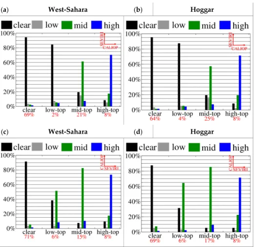
The average behaviour of the flux profiles in Figure 12, however, does not represent the different types of summer atmospheric circulation that appear in the daily profiles and in the flux profiles averaged in 15‐day steps over the West‐Sahara and the Hoggar (see Figures S2 and S3). To characterize these circulations the daily profiles are classified according to the sign of the flux convergence in the low troposphere, the mid‐ troposphere and the upper‐troposphere. The three vertical layers which are considered are: (1) surface to 850 hPa for the West‐Sahara and surface to 700 hPa for the Hoggar, (2) 700 to 500 hPa and (3) 400–70 hPa. Three classes are sufficient to classify more than 90% of the profiles (85% for the humidity convergence profiles over the West‐Sahara). Figure 13a displays the characteristics (the sign of convergence) of these classes (For the sake of clarity, the 400 hPa boundary has been removed from the figure). For the first two clas‐ ses labeled upper ascending profiles and subsiding profiles, convergence is positive in the upper part of the SABL (700 hPa–500 hPa layer in Figure 13a), while it differs in sign in the upper troposphere (400 hPa–70 hPa layer). For the third class, labeled SABL‐like profiles’ convergence is negative in the upper part of the SABL and positive in the lower part of the SABL (Figure 13a). Figure 13b shows the frequency of each class for mid‐top days, clear days and high‐top days for the West‐Sahara and the Hoggar. The frequency of profiles not classified is indicated by the gap between the top of the bar and 100%; at the top of the bars is indicated the frequencies of mid‐top days, clear days and high‐top days among the 854 days of observations. West‐Sahara Hoggar
Mid‐top days Clear days High‐top days (a)
(b)
Figure 13. (a) For each of the 3 classes of convergence profile, the pressure levels and the sign of convergence value (in‐ dicated by the convergence or divergence of the two arrows) used to perform the classification. (b) for the mass (Mass) and for the water vapor (WV), occurrence frequency distribution of the convergence profiles in the 3 type classification for mid‐top days, clear days and high‐top days in JJAS. Information is given for West‐Sahara (left column) and Hoggar (right column). For class 1 profiles labeled “upper ascending profiles” (Figure 13a, 17%/4% over the West‐Sahara/Hoggar) convergence is positive in the upper SABL and negative in the upper troposphere. Upper ascending profiles occur most frequently on high‐top days (Figure 13b). With these profiles, the mass flow rate ascends from the upper SABL to a higher level. In the lower SABL, on high top days the flow may diverge or converge while during clear days or mid‐top days the flow diverges (see Figure S5).
For class 2 profiles labeled “subsiding profiles” (Figure 13a) convergence is positive both in the upper troposphere and in the upper SABL and negative in the low SABL. These profiles are important only on clear days (Figure 13b) and they are more frequent for the mass than the moisture (17%/7% for mass and 11%/2% for moisture over the West‐Sahara and the Hoggar, respectively). During subsiding profile days, the mass flow rate is subsiding at almost all levels of the troposphere and when ascending flux is observed the flow rate is small (see Figure S6).
Class 3 profiles labeled SABL‐like profiles are frequent above the West‐Sahara (close to 60%) and very frequent over the Hoggar (85%). They reach their largest fre‐ quency on mid‐top days (Figure 13b). Their mean vertical profiles of vertical mass flux and their horizontal water vapor flux convergence profiles are given in Figure 14. On SABL‐like profile days the mass flow ascends from the low SABL to some level within the upper SABL and subsides above (Figure 14; see also the profile of the mass flow rate distributions in Figure S4). They correspond to the paradigmatic image of Thorncroft and Blackburn [61] and of Messager et al. [10], when above the Sahara the SABL is verti‐ cally developed. In the upper troposphere, the flows converge most of the time during mid‐top days and clear days. Upward flows can be observed but it is at levels well above the top of the SABL and the vertical mass flow rate is weak (see Figure S4). Exceptions are on high‐top days for which, mass flow diverges frequently in the upper troposphere (40% of the time). Above the Hoggar, on these days, the ascending vertical mass flow from the lower SABL reaches the upper troposphere.
During the season while the frequency of clear, mid‐top, and high‐top days vary (Figure 7), the frequencies of these three classes of profile vary. Figure 15 shows the fre‐ quency of each profile class for mid‐top days, clear days and high‐top days for 15‐day periods and for the West‐Sahara and the Hoggar. At the top of the bars, the frequencies of mid‐top days, clear days and high‐top days that are close to the number of days used to calculate frequency values, is indicated. Despite the large uncertainties induced by the small size of some samples, the behavior of the intra‐seasonal evolution of these fre‐ quencies allows some conclusions to be drawn. It should be noted that the total number of days in a period is equal to a maximum of 105 or 112 (7 times 15 or 16 days). For some periods, this number may be slightly lower due to a few days missing in the SEVIRI da‐ ta.
![Figure 1. Map of West Africa with relief, July position of sub‐tropical westerly jet (STWJ, blue line) [22], maximum monthly mean rainfall (dashed black line) [22], northernmost position of monthly mean rainfall > 25 mm (dotted red line) [22], the con](https://thumb-eu.123doks.com/thumbv2/123doknet/14778503.595079/4.918.277.565.126.341/figure-position-tropical-westerly-rainfall-northernmost-position-rainfall.webp)