Mathematical Programming 76 (1996) 131-154
Solving nonlinear multicommodity flow problems
by the analytic center cutting plane method
J.-L. G o f f m a,b,* ,2, j. Gondzio b,3, R. Sarkissian b, j._p. Vial b
a GERAD, Faculty of Management, McGill University, Montreal, Que., Canada H3A IG5 b Logilab. HEC, Section of Management Studies, University of Geneva, 102 Bd.Carl Vogt, CH-1211 Genbve 4,
Switzerland
Received 1 November 1994; revised manuscript received 1 November 1995
A b s t r a c t
The paper deals with nonlinear multicommodity flow problems with convex costs. A decompo- sition method is proposed to solve them. The approach applies a potential reduction algorithm to solve the master problem approximately and a column generation technique to define a sequence of primal linear programming problems. Each subproblem consists of finding a minimum cost flow between an origin and a destination node in an uncapacited network. It is thus formulated as a shortest path problem and solved with Dijkstra's d-heap algorithm. An implementation is described that takes full advantage of the supersparsity of the network in the linear algebra operations. Computational results show the efficiency of this approach on well-known nondiffer- entiable problems and also large scale randomly generated problems (up to 1000 arcs and 5000 commodities).
1. Introduction
T h e n o n l i n e a r m u l t i c o m m o d i t y f l o w p r o b l e m with s e p a r a b l e i n c r e a s i n g c o n v e x costs g i v e s rise to v e r y large n o n l i n e a r p r o g r a m s with linear constraints. It arises in the areas
• Corresponding author, e-mail: [email protected]
I T his research has been supported by the Fonds National de la Recherche Scientifique Suisse, grant #12-34002.92, NSERC-Canada and FCAR-Quebec.
2 This research was supported by an Obermann fellowship at the Center for Advanced Studies at the University of Iowa.
3 On leave from the Systems Research Institute, Polish Academy of Sciences, Newelska 6, 01-447 Warsaw, Poland.
0025-5610 © 1996 - The Mathematical Programming Society, inc. All rights reserved
132 J.-L. Goffin et a l . / Mathematical Programming 76 (1996) 131-154
of transportation networks, traffic assignment problems, telecommunication or computer networks, multi-item production planning, to name but a few applications. The decom- position
principle
of Dantzig and Wolfe [8] is well suited to the primal block diagonal structure of the constraints, even though the decompositionalgorithm
may show slow convergence on some, but not all, formulations or instances. The granularity of the formulation may have a significant impact on the effectiveness of the approach as noted and studied by Jones et al. [24] and Minoux [32].Three issues need to be settled to make for an effective algorithm:
• The formulation: how many commodities? Origin-destination problem, destina- tion specific (or-origin specific) problem or product specific problem, or in fact a combination of these three cases [24]?
• How to deal with the nonlinear objective?
• What solution concept to use in the master problem, to compute a set of prices that will be used to generate new proposals (columns) from the subproblems (oracles). The approach taken here uses the following answers to these three issues:
• The formulation: as fine a granularity (disaggregation) as the problem will allow. • Deal with the nonlinear objective by defining a subproblem (oracle, block,
convexity constraint) for each one-dimensional component of the objective. • Do not solve the master problem to optimality but compute an analytical center of
the set of localization (ACCPM: the analytic center cutting plane method) [15,3]. As in the Dantzig-Wolfe algorithm, our approach considers a restricted master program. This restriction is improved as new columns are added, either one at a time or in bunches. The analytic center of the set of localization is obtained by applying to the restricted master the de Ghellinck and Vial's variant [9] of Karmarkar's projective algorithm [25].
The purpose of our paper is to demonstrate that ACCPM is a viable tool for solving large non-linear multicommodity flow problems. Special attention has been paid to exploit structural sparsity in the restricted master. We conducted two different series of experiments. We first compared different levels of granularity on two well documented test problems; the finest granularity yields the best results by far. The second series of experiments pertained to random problems of various sizes - the formulation used the finest granularity. The results are very encouraging. The method is robust. Its behavior on the particular class of problems is very much alike what has been observed in different areas of application such as stochastic programming, multiregional planning, nonlinear programming, minmax problems. Our results provide further evidence that ACCPM is one of the method of choice for nondifferentiable optimization, especially for the nondifferentiable algorithms that arise in decomposition approaches to large scale programming.
Our specific contribution in this paper is twofold:
• our first contribution is to show that a full disaggregation has a dramatic effect on convergence; by this we mean a disaggregation on the OD pairs - the rationale here being that few shortest paths must appear in the optimal solution -
and
on each of the nonlinear cost arcs - the rationale being that cutting planes canJ.-L. Goffin et aL / Mathematical Programming 76 (1996) 131-154 133
approximate well functions of one variable. The impact of this disaggregation is a
considerable improvement not only of the ACCPM but also of Dantzig-Wolfe. • Second we propose an advanced implementation of ACCPM with this particular
application in mind. We refrained from undertaking a systematic comparison with other methods. We do not claim that our method is the best, but we claim that it is always competitive with the best, and that is is stable and robust, and not prone to slowing down as it is the case with some formulations of Dantzig-Wolfe decomposition.
There are, of course many other approaches to the linear or nonlinear multicommod- ity flow problem, many of them based upon variants of Dantzig-Wolfe decomposition, or dually, Kelley's cutting plane method or Benders's decomposition, all of which can
and have been interpreted in terms of nondifferentiable optimization.
The fully aggregated formulation (which corresponds to one convexity row) has been
used in many nondifferentiable optimization approaches: the subgradient method by Fukushima [12], the proximal bundle method of Lemar6chal [30] and Kiwiel [28], the bundle trust region method of Schramm and Zowe [36], the new bundle method of Lemar~chal, Nemirovskii and Nesterov [31], the affine scaling with centering bundle method of Hipolito [23], the dual ascent algorithm of Hearn and Lawphongpanich [21], and the restricted simplicial decomposition of Heam, Lawphongpanich, and Ventura [22], among many others. Most of these papers report results on the small nonlinear multicommodity flow problem NDO22.
Some of these algorithms do not extend easily to, or have not been tried with, a disaggregated formulation; the methods of [24] and [32] use disaggregation, but only in the linear case.
2. Problem formulation
The formulation of the multicommodity flow problem follows that of Minoux [32]. We assume that the arcs are not directed (thus flows can traverse arcs in both directions). The flows must then be added up in absolute value as they represent different commodities. This is typical of telecommunication networks. We could also admit that some arcs could be directed (one way), as is usually the case in transportation networks. For clarity's sake we will ignore this possibility.
We are given a graph ~ ' = ( ~ ' , .J~¢'), where ..~¢c{(s, t ) : s ~ T / , t ~ , s ~ t } and
m = card(~ "/') is the number of nodes; the arcs are directed, but the direction is selected arbitrarily. In order to formulate this as a nonlinear (or linear) program, the transpose of ,~¢ is defined as ,.~¢x- {(s, t): (t, s)~,~¢}. We also define T ( a ) - {(s, t): a = (t, s ) E
.at}. This simply associates to every directed arc (s, t) the arc with the reverse orientation (t, s); the two directed arcs a and T(a) represent the undirected arc {s, t}.
Clearly ,.a ¢x = T ( d ) . If the transposition map T(a) were to be defined on a subset of ,~',
134 J.-L. Goffin et al. / Mathematical Programming 76 (1996) 131-154
To define a nonlinear (or linear) programming formulation we thus use the aug- mented graph ~ = ( ~ z - , ..at--), where . ~ - " ~¢U..~ ¢T. We denote by n = c a r d ( , ~ ) the number of arcs and by N the m × n vertex-arc incidence matrix of ~'.
The set of commodities d r is defined by exogeneous flow vectors (supplies and demands) d i - - (ds) ` i E ~- that satisfy e ~ d i = 0 for i ~ d r , with e ~ a vector of ones. These flows must be shipped through ~'.
We denote by x i = ( x a ) , e ~ the flow of commodity i ~ d r. The feasible flows for commodity i are members of
s r i = { x i >1 0 : N x ~ = d i } .
Following the terminology in Jones et al. [24], the flow problem for commodity i is a single origin-single destination (SOSD) problem if d g has exactly one positive and one negative entry - the origin and the destination, respectively. If d i has one positive entry and several negative entries, we have a single origin-multiple destination problem (SOMD). We similarly can have a multiple origin-single destination problem (MOSD). These three formulations truly represent the same problem, in the sense that it is possible to aggregate SOSD into SOMD (or MOSD) and conversely disaggregate SOMD (or MOSD) into SOSD. This is easy to see as every SOMD flow can be disaggregated into a convex combination of trees (basis), and every tree-flow disaggregates uniquely into a sum of path-flows, see [24] and Rockafellar [35].
The case of multiple origin-multiple destination problem (MOMD) is somewhat different though, as this formulates the transportation of a generic commodity (gas, oil, cable television, aircraft, etc.). We will restrict ourselves in our experimentation to the origin-destination case (SOSD), even though the algorithm would be applicable to the MOMD, or the mixed M O M D - S O S D cases.
A linear cost vector c / is associated with the flows of each commodity. A nonlinear (or linear) cost is also charged on the total arc flow, where the total arc flow is
E, ej(x
+ XT(~)).i
A set of coupling arcs .J*¢' C~¢ comprises those arcs for which there is either a nonlinear cost or a limited capacity on the total arc flow.The nonlinear multicommodity flow problem can be formulated as min E
ci'rXi "~- E fa( Ya)
i .7
(1)
,(2)
i + xr(a)) ~< Ya V a ~,.Q¢" c,~¢', s.t. )--'. ( x a(3)
x / e 9 -/ V i e d r , (4)O<~ ya<~ i/~ V a e ~ ¢ ' c,.~¢'.
In this f o r m u l a t i o n the vector y = ( Ya)a e ~/' is meant to represent the j o i n t total arc-flow of a and T(a); in fact it is an upper bound to it, but of course y~ = Y'.ieu,(x i
"["X~(a))
a t the optimum if we assume that the cost function fo(y~) is strictly increasing. We further assume that the function f~(ya) is convex and the costs c" are nonnegative. This will ensure that the Lagrange multipliers (the prices of the coupling constraints) are nonnegative, and in fact positive in the ACCPM; from this follows that the shortest paths routines (the oracles) need not worry about negative or zero cost cycles.J.-L. Goffin et al./Mathematical Programming 76 (1996) 131-154 135
Constraints (3) and (4) are simple network and capacity constraints, respectively. Without (2), the problem is separable. Constraints (2) are named coupling since they coordinate the simple network problems. The nonlinear functions most used in practice
a r e :
• a power function fo(y~) = a~ yfo, with a~ > 0 and fl~ >i 1; • the delay function
f~(y~)= y~/(~/~ -yo).
Finally, we mention that the standard linear multicommodity flow corresponds to f~ - 0. It is then possible to combine (2) and (4) into
E ( Xi -l- XiT(a)) ~ ~l a
Va E ~',
to obtain the usual formulation:
min
~_,
ci'rx i i E J i s.t.E (x: + xr(~))<~ 7~
x i E ~ '~ Vi ~ r . Va Ez¢' c ~ ,(5)
(6)
(7)
3. The decomposition principle
Real-life multicommodity flow problems leed to very large scale programming problems. For instance a problem with 500 nodes, 1000 arcs and 5000 commodities in the SOSD formulation would lead to a nonlinear program with 2.5 × 10 6 constraints and 5 × 10⁶ variables; in the SOMD formulation it still remains a problem with 250000 constraints and 500000 variables. The difficulty in solving the problem as a single LP or NLP stems from the coupling constraints. The standard decomposition approach strives to separate the issues of finding flows for the individual commodities and of coordinat- ing the individual commodity solutions. In this section we shall briefly review the various elements of this well-known approach.
3.1. Lagrangian dual
The partial Lagrangian is obtained by the dualization of the coupling constraints, using Lagrange multipliers u = ( u , ) ~ d' and letting 7 = ( 7 a ) ~ ~,':
i + xr(,))
y~
(8)
Sa( x, y; u)= E cirxi + E f~( Y~) +
E ( x~
-
.
i E J aEA' aE,~ ¢ x iE~¢
We define
S a P ( x , y ) : = max Sa( x, y; u) (9)
136 J.-L. Goffin et aL / Mathemafical Programming 76 (1996) 131-154
and
SaD(u)
:= min . ~ ( x , y; u). (10)O<~ y~< y
The functions
~ e ( x , y) and .c.~D(u) are
respectively convex and concave. From the minmax theorem for convex programming:min S a P ( x , y) = m a x S : D ( u ) .
x i ~ i r i u ~ O
O~< y<~ 3'
So we can choose to solve (10) instead of (9), provided one is able to recover an approximate optimal primal solution ( x *, y * ) to (9) from an approximate optimal dual solution u* to (10). As the methods used generate both primal and dual solutions, this follows quite naturally from the algorithm.
3.2. Polyhedral approximation and linear relaxation
Column generation - or cutting plane - algorithms use the fundamental subgradient inequality for convex functions. Let us briefly recall the definition of the subdifferential. Let f be a convex function and let x be in the interior of the domain of f. The subdifferential set 0 f ( x ) of f at x is a nonempty compact convex set such that for any s ¢ ~ a f ( x ) and any y in the domain of f the following subgradient inequality holds:
f ( y ) >~f(x)
+ ~:T(y-- X).
Since - S : ° ( u ) is convex, we have that for each pair (u, fi) whose elements are in the domain of definition of .o-c¢ ° and each ~ in the subdifferential cg(-_o-cP°(fi)) at fi, the following inequality holds
__~O(u ) >/ _ . ~ o ( ~ ) + ~ T ( u _ 7 ) .
It is convenient to introduce the set - O ( - S : ° ( f i ) ) . So for each f e -O(--.Z~'D(fi)), the reverse inequality holds:
. ~ D ( u ) ~ . ~ o ( ~ ) + ~ r ( U _ ~).
The elements of - - O ( - 2 ° ( f i ) ) are sometimes named supergradients.
It is also known, by convex duality, that under the usual regularity conditions, S " ° ( u ) = min min ( S # ° ( f i )
+ ~ r ( u - ' ~ ) ) ,
where n' is the dimension of u or y, i.e., the cardinality of ~¢', or the number of coupling constraints.
This equality also holds if the minima are restricted to a dense countable subset of
{ ( ~ , - a ( - . Z ° ( ~ ) ) : ~ ~ ~'~
+ j "By using a finite subset of this countable dense set a polyhedral approximation to -.Z# D can be constructed and refined as this subset is expanded by further oracle calls.
It is thus possible to use the subgradient inequality to generate a polyhedral relaxation of the epigraph of the function - S aD. For instance, let u k, k = I . . . K, be a collection
J.-L. Goffin et al. / Mathematical Programming 76 (1996) 131-154 1 3 7
of points in the domain of S " ° and let ~k ~ _ 0 ( - ~O(fi~)) be an associated collection of supergradients. Then the set of pairs ( - z, u) satisfying
Z - - ( ~ k ) T U < . Z O ( U ~ ) - ( ~ ) T u ~ , k = l . . . ~,
is a polyhedral relaxation of the epigraph of _ ~ o . Thus the polyhedral function
k = l . . . . x
is an upper bound on Sa°(u), i.e., Vu e R ' .
Hence, the optimum of the linear programming problem (the linear relaxation, or the Dantzig-Wolfe point)
m a x { z :
z - ( ~k)a'u <~-c-~°(uk)-(
~ k)'rUk, k = 1 . . . K}, (11) provides an upper bound to the optimal value of S "°. We shall denote it 0~p.It is possible to localize more precisely the optimal point of . ~ o . Let 0i~f:= max
.c2O(uk)
be the largest value of S a ° recorded in the sequence. Clearly 0~ r is a lower bound for the optimal value of S a°. Moreover, any optimal point
(.~°(u*), u*)
lies in the so-calledlocalization set
= {( z,
u):
z>_- and~<,..f6'O(u
*) - ( ¢*)'ruk, k = l
...
K}.
(12)
3.3. Cutting planes: A prototype decomposition algorithm
The basic idea underlying cutting plane algorithms can be described as follows. Given a polyhedral outer approximation of the epigraph of the function, one selects a point u such that the pair (z, u), for some z, belongs to the localization set. The value
.oW°(u),
and an element ~ of the supergradient set, are then computed; a new validsupergradient inequality is added to the definition of the localization set. This new inequality either " c u t s " the localization set or is a support to it. The lower bound is updated and a new smaller localization set is obtained.
We can state formally the basic steps in the prototype cutting plane method. For the sake of simpler notations we drop the iteration index k. A localization set Sa~'~ ' and a lower bound 0in f are given.
Step 1.
Select (?., fi) ~_oca@~.138 J.-L. Goffin et al. / Mathematical Programming 76 (1996) 131-154
Step 3.
Update 0i. f by 0i. f := max{0i, f, .C.¢'°(fi)} and add the inequality z - ~ T u < S : ° ( ~ ) - ~:a-~to the definition of the localization set.
The process ends when the duality gap, 0,u p - 0i, f, falls below a given precision level. Step 1 of the prototype algorithm is usually called the master program. The way fi is chosen in the localization set characterizes the cutting plane method. Step 2 is problem dependent. It has been called an oracle, though the classical terminology in the Dantzig-Wolfe approach refers to subproblems.
4. Levels of disaggregation in the decomposition for multicommodity flow problems
In the case of the nonlinear multicommodity flow, the partial dual Lagrangian (10) is
.~°(u)= min ( ~
ciTxi'~ -E fa(Ya) + ~ U~(
Y'. (xia+X~(a))-ya)
)
xi~,~ri i~.Y" a~.a:' a ~ / ' ~ i E J O~y<~ y
= min •
(Ci+u)Txi+
minE (f.(Ya)--u~Y~)
x,~.~r i i~.)r 0~<y~< y a~.~¢,
= E min
(ci+u)Xx'+ ~,
min (f~(ya)-u~y~).
i ~ . J "xiEoq-i aEA' O<Yo<~ ~a
The computation of the function
_oW°(u)
and of a supergradient separates into easily computable functions:-Z#°(u) = E .o~'(u) + Y'. .~'~(u),
(13)i ~ , f a E ge"
where each
.oc:/(u) = m i n ( c i " ~ u ) T x i (14)
is the solution of a shortest path problem with nonnegative costs c i + u, and where, abusing notation,
uTx i
meansF..~s:,u.(x ~
+ Xr(o)), whilei
. ~ a ( u ) = min
(f~(y~)-u~y.)
(15)O~Ya~< Yo
is a one-dimensional convex program whose solution can usually be given analytically. It should be noted that if the costs c ~ do not depend on the commodity i, then only
one
shortest path problem between all pairs of nodes needs to be solved.It is interesting to note that in the case of linear costs, fa - O, the Lagrangian dual is
. ~ ° ( u ) = ~2
min.(ci +u)Txi + ~_. min (--u.y.).
(16)J.-L. Goffin et al. / Mathematical Programming 76 (1996) 131-154 139
It is important to note that, in the usual linear case (5), the function 2 ° differs in a very significant way from the partial dual associated to the (nonlinear) multicommodity flow formulation (1). Letting v. be the Lagrange multipliers there one gets
2 1 ° ( v ) =
Y'~
min(ci'~u)Txi--uT~/,
(17)The functions 2 ° and ..?'1 ° appear to be the sum of hopefully simpler functions. The simple structure can be exploited to yield various level of disaggregation. Each level generates its o w n set of subgradient inequalities.
4.1. No disaggregation: Single cuts
I f we do not take advantage of the additive structure of 2 °, we obtain a supergradi- ent o f 2 ° at fi as follows. Let x(fi) and y(fi) be optimal solutions of problems (14) and (15) for a value fi of the Lagrange multiplier. The supergradient of
2 ° ( u )
at fi = u is given by the coefficient o f ft. in (13), i.e.,~a = E (xi("~) + X!r(a)(-u))--Ya('u))"
~ is zero, as the subproblems Note that at least one of the components of x . or Xr(.)
compute shortest paths or trees.
In the case o f linear costs it is interesting to compare the two formulations (16) and (17). In the former case the function ]Ea~ ~,,..oc~"(u) has a superdifferential at u = 0 with 2 ' extreme points while in the latter case - v ' r y is differentiable and has a unique supergradient - y.
Practitioners have always noticed that the additive structure of 2 1 ° can be used for a variant of D a n t z i g - W o l f e decomposition, which is sometimes effective.
4.2. Full disaggregation: Multiple cuts
The linear case
Recall that
2 g ( v ) = E 2 / ( v ) -
A disaggregated LP relaxation can be defined as SolO(v) = - - v r y + • m a x { z i :
Zi~*~i(o)},
i ~ J xi
where
2 i ( v ) = rain
( c i + v ) r x i.
(18)x,~sr'
Each function 2 i has its own support s ¢ i =
x i
at a point ~. Now the proposals ~:" depend on whether the formulation is SOSD or SOMD; in the former case the proposals are path-flows, in the latter they are tree-flows.140 J.-L. Goffin et aL,/ Mathematical Programming 76 (1996) 131-154
As clearly shown in [24] the most disaggregated formulation, i.e., the SOSD formulation using path-flows, is the most effective one. Only a few proposals are needed for each of the component functions to define them accurately. The SOMD or tree-flow formulation creates exponentiality in the number of extreme points of the subdifferen- tials.
In this disaggregated formulation it is possible to introduce a cut for each i E J . To this end we introduce variables zi, and z = ( z i ) ~ j . We define the LP relaxation in the extended space I~ n'+ IJl+ i by
max z subject to
z= E Zi--vT3 ',
(19)Zi--(~ik)Tv<<..~i(V k ) - ( ~ : i k ) T v k ,
i E I ,
k = l .... K
while the set of localization becomes(( z, z,,
o e,z= -oTr+ E z,,
Z i - (eik)Tv<~c.c.c.c.~i(vk) --
(~:it)Tv',i e l ,
k = 1 . . . . K}. (20)The nonlinear case
In the nonlinear case the disaggregation needs to go further; we have --~°( u ) = E S ( u ) + E ~ ° ( u ) .
i E J r a~A'
We may choose a partial disaggregation
c-~°(u)=max{zo:zo <~ C
--°oPt(u)} + Cmax{zi'zi<'---gF'(u)},
Zo a ~ ¢ , iE.Y zi
but the finer granularity of
_ ~ O ( u ) = )-"
max{zo:z <~SaO(u)}+ ~_, max{zi:zi<-~-c-c-~i(u)}
a ~ d ' z, i ~ J z~
turns out to be
significantly
more effective.We define the LP relaxation in the extended space I~ 2n'÷ IJl+ I as n' = I ,J~¢' l, by:
m a x z
subject to
Z = E Zi"I- E Za, i ~ J aEA'
T k Zi__ ( ¢ik)Tbl ~.~c~i( u k) _ ( ~ i k ) U ,
zo- ( e"')'u
- (
i ~ J , k = 1 . . . . K, a ~ , ~ ¢', k = l . . . . K,
J.-L. Goffin et aL / Mathematical Programming 76 (1996) 1 3 1 - 1 5 4 141
while the set of localization becomes:
~e~'K = (( z, z~, ZA', U)" Z >/ 0~f,
z= E z , + Ezo,
i E J i ~ A '
Z i - - ( ~ i k ) T l d ~ . f ~ i ( I d k ) - -
(~'k)Tuk, i ~ I , k= 1 .... K,
Za-- ( ~Qk)Zu <~.c.~"( Uk) -- ( ~k)Tuk, aEa¢', k= 1 .... K}.
(22)The motivation here is that it is easy to approximate the functions ~ i in the SOSD case, as few proposals (supergradients) are needed to approximate _9 ~i accurately hut that is also easy to approximate the functions .9 ~ by cutting planes as they are functions of one variable only.
Note that the supergradient ~ ;k represents a shortest path between the origin and the destination of commodity i, that carries the total flow of commodity i. The supergradi- e n t
~ak
has one nonzero component sod k = _yffk.There is of course one drawback to this finest of granularities: the restricted master program - the dual of (22) - has as many convexity rows as there are coupling arcs
and
commodities ( 1 5 1 + I se' I). Fortunately, those can be handled very efficiently by the GUB technique as will be shown in Section 6.1. Another point to note is the fact that the supergradients are sparse, as ~:; are paths and s ca have only one nonzero component.5. The analytic center cutting plane method (ACCPM)
There exist several reports on the principle of the method [15] and on its implementa- tion aspects [16,4,5]. For clarity's sake we provide here a short description of ACCPM. The problem of interest is the computation of the analytic center of the set of localization. This set is defined by a system of inequalities such as (21) or (22); in order to make it compact, we add artificial bounds u ~< M on the Lagrange multipliers. We already noted that in our formulation of the multicommodity network flow problems the multipliers are nonnegative. (The box constraint 0 ~< u ~< M clearly compactifies the domain.) The analytic center is the unique maximizer of the product of the slacks to each of these inequalities (or equivalently, the sum of their logarithms).
Different interior point methods can be used to compute the analytic center. In ACCPM we choose a variant [9] of Karmarkar's projective algorithm [25] and apply it to the dual of (21) (or (22)). The analytic center, or its approximation, is obtained by simple duality.
Let us stress that the dual of (21) (or (22)) is the restricted master program of the Dantzig-Wolfe algorithm. This linear program has a special structure. Individual columns in it correspond to cuts (supergradients) generated by a commodity or by a
142 J.-L. Golf in et al. / Mathematical Programrnhlg 76 (1996) 131-154
coupling arc. The columns associated with the same commodity are linked by a convexity constraint and so are the columns corresponding to a given coupling arc; hence a GUB structure. In addition to these columns, there are unit vectors correspond- ing to the box constraints 0 ~< u < M.
In a typical iteration, new columns are added after the analytic center of the current localizaton set has been computed. The localization set is updated and a new analytic center is computed. In order to cut down the computational effort, one should be able to make use of the previous analytic center as a warm start. This is known to be a challenge for any interior point method. In the projective method we use, the addition of the cuts in the localization set amounts to the introduction of new columns, i.e., variables that must be given an initial value zero to maintain feasibility, thereby violating the fundamental interior property requirement of the method. To handle this case a special technique has been devised proposed in [33]. (See [15] for the principle and [4],[5] for a detailed description.) Note that for a nonlinear multicommodity flow problem, the number of potential new columns at each iteration is the number of commodities plus the number of coupling arcs, a considerable number for problems with many commodities or many coupling arcs.
6. Implementation of ACCPM
The ACCPM approach presented in previous sections has been implemented and applied to solve two practical (and well documented in the literature) nondifferentiable optiinization (NDO) problems: NDO22 and NDOI48 and several large randomly generated problems. As we were encouraged by the results of earlier experiments [15,16], we have decided to prepare a specialized sparsity-exploiting implementation of the method dedicated to real-life large scale multicommodity network flow problems. This section addresses several issues of our implementation.
6.1. Projective algorithm in the master problem
As explained before a single outer iteration consists of finding an approximate analytic center for a (modified) set of localization. This is done by the projective algorithm. The bulk of the work in a single iteration of it (as in a single iteration of any other interior point method [19]) is clearly computing the orthogonal projection of a vector onto the null space of a scaled linear operator. Let A denote this linear operator (the LP constraint matrix) and Y denote a diagonal scaling matrix. We need to compute the orthogonal projection of a vector onto the null space of AY and this effort is dominated by the inversion of the matrix
J.-L. Goffin et al. / Mathematical Programming 76 (1996) 131 - 154 143 The matrix A shows a lot of special structure in itself resulting from box constraints imposed on dual variables, our approach to dealing with nonlinear objective term and, finally, GUB constraints coming from the decomposition approach.
hT
. . . Gp - I G~eY
A = (24)C = Y'~
GiY~G
~
+ Y~ + Y~ + d i a g ( h r y ~ h j ) ,
i=1B,=(G,Y~,e,.G2Yo22e2 . . . GpY~pep),
B 2 = d i a g ( h r y ~ f j ) ,
D, =diag(eTy~ ei),
= (27)(28)
(29) (30) (31) where PHere Y is a (presumably dense) column resulting from the transformation of the problem to the form required by the projective algorithm [9], each column of
G i
characterizes a feasible path (one supergradient ~ik in the notation of (22)) for the demand of commodity i, i = 1 . . . p, hi, j = 1 . . . n, are vectors built of supergradients corre- sponding to nonlinear part in the objective ( ~ k in (22)). Next,e i, i = 1 . . . p and fj,
j = 1 . . . n, are now vectors of all ones of appropriate dimensions (GLIB constraints). In order to solve large scale problems and to reach maximum efficiency in the implementa- tion, we have to exploit the special structure of A. We discuss below how this can be done. Assume the scaling matrix Y has been partitioned accordingly to (24):Y = diag(Yv,
Yn,, Yn2' Yc, . . . YG' Yh,. .... Yh.)"
(25) Then (23) becomesC B I B 2
AY2A T = H
+ , y y 2,yT ~. n T O l 0 4- TY~T T, (26)144 J.-L. Goffin et aL / MathematicaI Programraing 76 (1996) 131-154
~
From the (26):
It is also convenient to introduce the matrices
I
Column 3' of (24) is supposed to be dense. If not taken into account separately, it would completely destroy the sparsity of A Y 2AT. It is best to view it as a rank-one correction to H and handle it by the Schur complement mechanism [7,14]. Assume that we have computed a symmetric (sparse) factorization
L A L T. (33)
Sherman-Morrison-Woodbury formula we obtain the following inverse of
(
l
)
( A y 2 A T ) - t = L - V A - I / 2 I I + v T A _ I v V V T A - I / Z L -z where v = L-IYz, y . (34)(35)
The above formula thus yields that, having done the preparation step (35), we can solve any equation with Ay2AT: this involves one forward transformation with L, one backsolve with L T and a few scalar products. Before we move on to the description of our approach to the computation of the factorization (33), let us comment on the dimension of matrix H in (26). C is an almost completely dense square matrix which size is the number of arc flow constraints. D l and D z are diagonal matrices of sizes equal to the number of commodities p and the number of arc flow constraints n, respectively. NDO148, for example, (see numerical results section) has 148 arc flow constraints and 122 commodities, so H has dimension 2n + p = 418; this could be handled by any general purpose sparse Cholesky factorization code. However, we expect computational advantages as well as obvious storage savings from avoiding its explicit formulation. Instead, we propose a specialized block decomposition technique for its inversion. The whole diagonal block D is pivoted out first, as this operation introduces no fill-in:.:(,
0
o°)('o
0),
Next, we build the dense symmetric matrix S, and compute its triangular factorization
S = C - B D - I B T = LoDoLVo .
We then obtain the required representation
I 0 D ] ~ D - I B T
(37)
J.-L. Goffin et aL /Mathematical Programming 76 (1996) 131-154 145
which is basically the same as (33), except that L and A are decomposed into smaller easily invertible blocks. Summing up, the solution of an equation with Ay2A T needs two solves with L and one with L T, where
L = ( L°0 BD-')I (39)
is a block upper triangular matrix. It also needs several additional inner products. The main computational effort in finding representation (38) consists in creating and decomposing matrix S in (37). To avoid explicit formulation of BI in S we represent the term B~DT~B~ as the weighted sum of the outer products of columns b i of B~. Thus we have for S,
~ l | T ¿B T"
S = C - - ~ b i b i - B2D f (40)
i= I i
(Recall that S is dense so we do not bother about the order in which simple products in
bib f are accumulated.) A column of B I is thus built and forgotten just after its contribution to (40) has been added. B 2 is a diagonal matrix and its contribution to (40) is the same. Implicit handling of B t leads to clear storage savings. The only part of H that has to be stored is matrix C which is later rewritten with S and finally replaced with a factorization (37). Its size is equal to the number of arc flow constraints, and thus, is known in advance.
In addition to the construction of S, the matrix B is used again in solves with L and L T. The implicit handling of B~ here also leads to computational time savings, due to the special structure of the G i matrices. This will not necessarily be the case in other ACCPM applications as will become clear after the presentation of our approach to the handling G~ matrices in Section 6.3.
Let us finally address the issue of stability in computing orthogonal projections. In our experiments we observed excellent accuracy, which seems to be a structural feature of the approach. First, the matrix (24) has full row rank even after removal of the first column y. Second, all GUB constraints are orthogonal to each other. The presence of diagonal term Y 2 + y 2 in (27) prevents excessive spread of the pivots in the factoriza- r/l "1/2 tion (37). Consequently, the factorization (33) is stable and so is the rank-one update (26) used to deal with dense column T- This situation is in contrast to general linear programming [19] for which a removal of dense columns may lead to a rank deficiency of Sherman-Morrison-Woodbury update.
6.2. The oracle
Each subproblem consists in finding a minimum cost flow between an origin and a destination node on an uncapacited network and it can be formulated as a shortest path problem. As the network is expected to be sparse, Dijkstra's d-heap algorithm is a suitable solution method. Our implementation follows the description of [1]. The basic
146 J.-L. GoJ~n et ul. / Mathematical Programming 76 (1996) 131-154
step of Dijsktra's algorithm consists of an update of two independent data structures: a set of nodes S a for which the shortest path has already been determined; and a set of all neighbours of S ~ (nodes that are adjacent to a node in S'0. In a single iteration, Dijsktra's algorithm chooses one node from the set of neighbours and adds it to S a. To accelerate the search in a subset of neighbours, nodes are stored in a form of a tree (d-heap). Once a node is chosen, the list is updated accordingly.
The reader interested in a more detailed description of Dijktra's algorithm and its efficient implementation is referred to [ 1 ]. Let us mention, however, that its application undoubtly contributed to the overall efficiency of the ACCPM approach on this particular class of multicommodity network flow problems. In fact, even with a large number of subproblems to be solved at every cutting plane iteration (see the numerical results in Section 7), the time needed to find a minimum cost flow seldom exceeded 10% of the total computational time.
6.3. Data structures f o r cuts
Every call to the ith shortest path subproblem can add a new cut, i.e., a new column to the matrix G;. Each subproblem consists of finding a minimum cost flow between two nodes. In many practical applications, this path involves only a few arcs. As a result, every column has only a few nonzero elements. These nonzeros have all the same value gi for each commodity i. Thus we may write
G i = giGio, (41)
where Gi0 is a 0 - 1 matrix that can be stored in a compact form involving half length integers. Moreover G~0 is usually very sparse. We refer to it in every solve with L of (39) and in the computation of (40). Each such reference creates a single column of B~,
bi _ - G i Y d e i , 2 (42)
possibly scaled by some factor. We take advantage of the form (41) and replace the above equation with
bi= Gio( giY~ ei). (43)
We thus reduce the number of necessary multiplications from the number of nonzero entries of G~ to the number of its columns (these multiplications need to be done only once in a single iteration of the projective algorithm). The remaining arithmetic operations in (43) are additions that would also have to be done if (42) had been used. The matrices G i grow in subsequent iterations of the ACCPM algorithm so the most suitable data structure to remember them is a collection of sparse columns (see, e.g., [10, Chapter 2]). Let us finally observe that replacing (42) with (43) is advantageous only if these columns are very sparse and their number is not excessive. Fortunately, both these conditions were always satisfied when solving multicommodity network flow problems.
J.-L. Goffin et aL / Mathematical Programming 76 (1996) 131-154 147
7. Numerical results
An implementation of ACCPM algorithm has been written in C (except for the Cholesky factorization that comes from LAPACK of Andersen et al. [2] and is written in FORTRAN 77). The code has been run on a POWER PC workstation (type 7011, model 25T) with 64MB of virtual memory. It was compiled with the AIX XL C + + and FORTRAN 77 compiler with a default optimization level (-O option). Several multicom- modity network flow problems have been solved with ACCPM, each to a six-digits relative accuracy of the optimal solution.
7.1. Impact of disaggregation
Our first series of tests were performed on two practical, well documented, standard nondifferentiable problems NDO22 and NDOI48 from [13]. See Table 1 for their statistics.
We used two different levels of granularity: cuts are fully aggregated and fully disaggregated.
In Tables 2 and 3, we report detailed information on the influence of various levels of aggregation on the efficiency of ACCPM and Dantzig-Wolfe (DW) implementations, respectively. The tables report: the number of outer iterations, NITER, the number of inner iterations, Newton steps (or simplex pivots in the case of DW), the number of cuts (supergradients) added and the solution time. A simple test was used to check not to duplicate the existing cuts. (It was applied to the linear parts only.) Note, that in a case of full aggregation, each iteration generates one cut while in the case of maximum disaggregation, each iteration generates p cuts for the nonlinear part ( p = 22 and p = 148, respectively) and at most n cuts for the shortest path part (n = 23 and n = 122,
respectively).
As mentioned earlier, the efficiency of ACCPM depends mainly on the number of interior point (Newton) iterations which does not seem to vary much with the number of subgradients added at every outer iteration. The disaggregated version of ACCPM accumulates about one cut per subproblem at every outer iteration, many more than in classical aggregate NDO approaches. Note, that the number of outer iterations or, equivalently, calls to oracle, corresponds to the number of objective function evaluations (a usual measure of efficiency in nondifferentiable optimization [27]).
Summing up, ACCPM did pretty well, finding an accurate solution in a number of iterations proportional to the number of coupling constraints n', in the case of aggre- gated formulation and O(1) in the disaggregated formulation.
Table 1
N D O p r o b l e m s statistics
P r o b l e m N o d e s A r c s C o m m . O p t i m u m
N D O 2 2 14 2 2 23 - 103.412017
148 J.-L. Goffin et al./Mathematical Programming 76 (1996) 131-154
Table 2
Efficiency of ACCPM on nonlinear NDO problems
Disaggr. NDO22 N DO 148
NITER N e w t o n CUTS Time N I T E R N e w t o n CUTS Time None 138 186 138 1.37 857 1011 857 558.08 Maximum 14 50 353 0.51 16 81 2649 16.15
In contrast, the behavior o f D a n t z i g - W o l f e algorithm depends much on the aggrega- tion o f cuts. F o r an advanced implementation o f D a n t z i g - W o l f e algorithm see, e.g., [1 l] and [24]. W h e n multiple cuts are used, both A C C P M and D W work similarly, although A C C P M turns out to be about two times faster on larger, NDO148 problem. W h e n fully aggregated cuts are added, D W looses much o f its efficiency and performs poorer than A C C P M . In particular, D W was unable to solve N D O I 4 8 problem in a reasonable time. It stalled with a relative precision of about 20%.
7.2. A C C P M on large scale problems
Let us now analyse the efficiency o f the method on large scale nonlinear multicom- modity network flow problems. A c c o r d i n g to our knowledge, there is no public d o m a i n collection o f large scale multicommodity network flow problems. Most o f problems reported in the literature come from practical applications and are proprietary. We thus decided to generate randomly a wide class o f such test problems. Below we briefly describe the way in which it is done.
The program generates a m u l t i c o m m o d i t y flow problem with n c commodities on a graph that has n n nodes and n a arcs. (The numbers n c, n n and n a are user supplied.) The graph has a two-level structure. Its lower level consists o f n b - 1 independent (connected) subgraphs. Each o f them has roughly speaking the same number o f nodes and arcs but their structure is randomly generated. The total number o f nodes in these subgraphs is n n.
F o r every lower level subgraph a node is chosen (call it connector) and another, connected, randomly generated graph is spanned on the set o f connectors. The number o f arcs in this higher level subgraph is chosen in such a w a y that the total number o f arcs in the network is equal to a prescribed value n a. F r o m this construction, the resulting graph is connected. It contains n b blocks: n b - 1 of them are completely
Table 3
Efficiency of DW on nonlinear NDO problems
Disaggr. NDO22 NDO 148
NITER Pivots C U T S Time NITER Pivots CUTS Time None 582 4239 582 23.35 > 10000 ? 10000 > 50000 Maximum 14 343 630 0.46 16 7350 4320 27.66
J.-L. G¢~n eta I. / Mathematical Programming 76 (1996) 131 - 154
Table 4
Statistics of randomly generated problems
149
Problem Blocks Nodes Arcs Comm.
Random I 4 60 140 100 Random2 4 60 1 40 500 Random3 4 60 1 40 2000 Random4 4 100 150 120 Random5 5 100 300 200 Random6 I 0 100 300 200 Random7 10 200 400 200 Random8 I 0 200 400 500 Random9 10 200 500 500 Random I 0 I 0 200 500 1000 Random I 1 I 0 200 500 3000 Random 12 I 0 300 600 1000 Random 13 10 300 800 1000 Random 14 10 400 800 2000 Random 15 15 300 1000 4000 Randoml6 10 300 1000 1000 Random 17 I 0 400 1000 2000 Random 18 15 400 1000 3000 Random 19 15 400 1000 4000 Random20 15 400 1000 5000 Random21 15 500 1000 3000 Random22 15 500 1000 4000
independent lower level subnetworks and the last one defines links between them. Each block has the same n u m b e r s of nodes and arcs, n n / n b and n a / n b, respectively (unless n n and n a are not multiples of nb).
In the next step, n c o r i g i n - d e s t i n a t i o n pairs of nodes are randomly chosen. A single path flow is then generated between each o r i g i n - d e s t i n a t i o n pair. Next, the sum of all flows passing through a given arc is computed and increased with some (safety) positive n u m b e r to define a capacity of the arc. For such capacities the problem has well defined feasible and optimal solutions.
Let us mention that our generator of nonlinear multicommodity network flow
4
problems is available for research purposes.
We have used this generator to produce a wide class of test problems that differ in the size and in the structure of the network. As we have observed consistent good efficiency of the A C C P M approach on these problems, we do not report all results obtained but restrict ourselves to a representative subset of them. Table 4 collects information on these test problems. For every problem, it reports several characteristics of the graph structure, namely: the n u m b e r of subgraphs, the n u m b e r of nodes, the n u m b e r of arcs and the n u m b e r of commodities.
The problems collected in Table 4 are listed in increasing order of the n u m b e r of arcs n. Recall that this n u m b e r determines the size of matrix S of (37) so it is the most
150 J.-L. Go ffin et al./Mathematical Programming 76 (1996) 131-154
Table 5
Efficiency of ACCPM on randomly generated problems
Problem NITER N e w t o n CUTS CPU time
total paths t F t o total
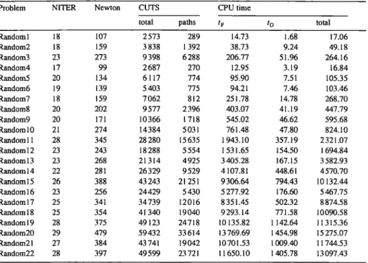
Random 1 18 107 2 573 289 14.73 1.68 17.06 Random2 18 159 3 838 1 392 38.73 9.24 49.18 Random3 23 273 9 398 6 288 206.77 51.96 264.16 Random4 17 99 2687 270 12.95 3.19 16.84 Random5 20 134 6117 774 95.90 7.51 105.35 Random6 19 139 5 403 775 94.21 7.46 103.46 Random7 18 159 7 062 812 251.78 14.78 268.70 Random8 20 202 9 577 2 396 403.07 4 I. 19 447.79 Random9 20 171 10366 1718 545.02 46.62 595.68 Randoml0 21 274 14384 5031 761.48 47.80 824.10 Randoml I 28 345 28280 15635 1943.10 357.19 2321.07 Randoml2 23 243 18288 5554 1531.65 154.50 1694.84 Random 13 23 268 21 314 4 9 2 5 3405.28 167.15 3582.93 Randoml4 22 281 26329 9529 4107.81 448.61 4570.70 Random 15 26 388 43243 21 251 9306.64 794.43 10 132.44 Randoml6 23 256 24429 5 4 3 0 5277.92 176.60 5467.75 Randoml7 25 341 34739 1 2 0 1 6 8351.45 502.32 8874.58 Randoml8 25 354 41340 1 9 0 4 0 9293.14 771.58 10090.58 Randoml9 28 375 49 123 24718 10 135.82 1 142.64 11 315.36 Random20 29 479 59432 33614 13769.69 1 454.98 15275.07 Random21 27 384 43 741 19042 1 0 7 0 1 . 5 3 1 0 0 9 . 4 0 11744.53 Random22 28 397 49599 2 3 7 2 1 11650.10 1 405.78 13097.43
important factor in evaluating A C C P M ' s computational effort (every inner iteration of the method requires computing one Cholesky decomposition of S; this is done in about
~n' 3 flops
[18]).
Let us observe that the numbers given in Table 4 " h i d e " the large size of the problems solved. The linear version of the R a n d o m l 0 problem, for example, in an equivalent compact LP formulation, would involve 200 blocks of 1000 constraints of commodity flow balance at each node and 500 coupling constraints of total flow capacity on the arcs. This formulation comprises 200 * 1000 + 500 = 200 500 constraints and 2 * 5 0 0 * 1 0 0 0 = 1 0 0 0 0 0 0 variables. The reader interested in the influence of the multicommodity flow problem formulation on the efficiency of different solution methods is referred to [24].
Table 5 collects data on the solution of randomly generated problems. We report in it: the n u m b e r of outer iterations, NITER, the n u m b e r of i n n e r iterations, Newton, the total number of cuts (subgradients) added through the whole solution process, the number of shortest path type cuts and the C P U time (to reach a 6-digit accurate solution on a P O W E R PC computer). To give a bit of an insight into the A C C P M ' s behavior, Table 5 additionally reports the time spent in the factorizations of S (dominating term in the master), tp, and the time spent in the oracle, t o.
A n analysis of Table 5 results clearly indicates that the most computationally expensive part of A C C P M consists in building and factorizing matrix S (see Eqs. (37)
J.-L. Goffin et ak / Mathematical Programming 76 (1996) 131-154 151
and (40)). Apart from the predicted cubic dependence of this effort on the number of arc flow constraints n, we also note considerable influence of the number of commodities, specially if n is not excessively large. Such an influence is observed on problems 1, 2 and 3 which differ only in the number of commodities (100, 500 and 2000, respectively). It is considerably less important for larger n (compare, for example, times for problems R a n d o m l 6 through Random20) although the total number of cuts varies linearly with the number of commodities. The time spent in subproblems usually varies between 5 and 10% of the total CPU effort and depends little on the number of commodities, which proves the high efficiency of Dijkstra's d-heap algorithm for this class of problems.
Let us observe that except for problems with a very large number of commodities, the average number of Newton steps required to approach a new approximate analytic center of the localization set is about 10. For problems with a large number of commodities many more cuts are added at every call to the oracle. Consequently, more significant changes are made to the localization set and the projective algorithm needs more iterations (up to 20, in the average) to approach the new approximate analytic center. This is a possible place for further improvements.
Finally, we would like to comment on the number of subgradients added during the solution process. The number of subgradients corresponding to the shortest paths shows uniform linear dependance on the number of commodities: from 3 cuts per commodity on smaller problems up to 7 cuts per commodity on larger ones. The total number of subgradients counts also the cuts resulting from the nonlinear term in the objective. It thus depends much more on the structure of the network and on how tight the arc capacity constraints are. Our experience indicates that, in practice, this number also grows linearly with the number of commodities.
Our last experiment aims at showing the trade-off between the required relative precision of the optimum and the time needed to reach it for the problem Randoml0. In Table 6 we report numbers of outer and inner iterations, the number of subgradients (cuts) added, and the CPU time required to reach a given number of the exact digits of the optimum.
The results collected in Table 6 show that it takes much time to build the first complete description of the localization set and to reach at least one digit exact solution.
Table 6
Trade-off between an accuracy and an efficiency of ACCPM for Random 10 problem
Accuracy NITER Newton CUTS CPU time
total paths 1 digit l I 140 10 195 4946 433.59 2 digits 13 180 11 145 5030 550.53 3 digits 15 208 11974 5031 628.97 4 digi ts 17 230 12 784 5031 692.02 5 digits 18 245 13 186 5031 739.71 6 digits 21 274 14 384 5031 824.10 7 digits 22 293 14783 5031 896.93 8 digits 23 335 15 182 5031 1016.69
152 J.-L. Go ffin et a l . / Mathematical Programming 76 (1996) 131-154
(This part of the optimization process takes about 50% o f the effort to solve the problem to 6 digits.) However, once the optimum has been approximately localized, the next digits (up to 8) can be achieved relatively fast with an effort that is almost linear with the number of digits required in the optimum. The method deteriorates if the academic precision 10 -9 is required. Recall that practitioners are normally satisfied with a two or three digit solution.
Up to the level o f accuracy of 10 -6, the projective algorithm involves from 10 to 15 iterations per outer iteration. For higher level of accuracy ( < 10-6), this number increases to 20 and 40. We believe that this is essentially due to insufficient accuracy in the computation of the search direction. Despite an iterative refinement procedure the Cholesky factorization attains its limits.
8. Conclusions
We have presented a specialized version of the analytic center cutting planes method for nonlinear multicommodity flow problems. We have discussed the influence of different aggregation/disaggregation techniques on the behaviour of the method and presented a detailed description of its sparsity-exploiting linear algebra kernel that ensures its high efficiency.
Computational experience showed the m e t h o d ' s ability to solve fast even very large scale problems on a workstation with 64MB o f memory. The method has been tested on public domain collection of large scale problems and two small, nondifferentiable optimization problems known from the literature.
The analysis o f numerical results shows promise for A C C P M to become a competi- tive method for nonlinear multicommodity flow problems.
Acknowledgement
The authors thank Olivier du Merle for many helpful suggestions concerning the efficient implementation of A C C P M and for running the D a n t z i g - W o l f e algorithm.
References
[1] R.K. Ahuja, T.L. Magnanti and J.B. Orlin, Network Flows (Prentice-Hall, Englewood Cliffs, N J, 1993). [2] E. Anderson, Z. Bai, C. Bischof, J. Demmel, J. Dongarra, J. Du Croz, A. Greenbaum, S. Hammarling, A. McKermey, S. Ostrouchov and D. Sorensen, LAPACK Users" Guide, (SIAM, Philadelphia, PA, 1992). [3] D.S. Atkinson and P.M. Vaidya, "A cutting plane algorithm that uses analytic centers," Mathematical
Programming 69 (1995) 1-43.
[4] O. Bahn, J.-L. Goffin, J.-P. Vial and O. du Merle, "'Experimental behaviour of an interior point cutting plane algorithm for convex programming: An application to geometric programming," Discrete Applied Mathematics 49 (1994) 3-23.
J.-L. Go)y[n et aL /Mathematical Programmhzg 76 (1996) 131-154 153 [5] O. Balm, O. du Merle, J.-L. Goffin and J.-P. Vial, " A cutting plane method from analytic centers for
stochastic programming," Mathematical Programming 69 (1995) 45-73.
[6] I.C. Choi and D. Goldfarb, "Exploiting special structure in a primal-dual path following algorithm,"
Mathematical Programming 58 (1993) 33-52.
[7] R.W. Cottle, "'Manifestations of the Schur complement," Linear Algebra and its Applications 8 (1974) 189-211.
[8] G.B. Dantzig and P. Wolfe, "'The decomposition algorithm for linear programming," Econometrica 29 (4) (1961) 767-778.
[9] G. de Ghellinck and J.-P. Vial, " A polynomial Newton method for linear programming," Algorithmica 1 (1986) 425-453.
[10] I.S. Duff, A.M. Erisman and J.K. Reid, Direct Methods for Sparse Matrices (Oxford University Press, New York, 1987).
[ll] J.M. Farvolden, W.B. Powell and l.J. Lustig, " A primal partitioning solution for the arc-chain formulation of a multicommodity network flow problem," Operations Research 41 (1993) 669-603. [ 12] M. Fukushima, "'On the dual approach to the traffic assignment problems," Transportation Research B
18 (1984) 235-245.
[13] E.M. Gafni and D.P. Bertsekas, "Two-metric projection methods for constrained optimization," SIAM
Journal on Control and Optimization 22 (6)(1984) 936-964.
[14] P.E. Gill, W. Murray, M.A. Saunders and M.H. Wright, "Sparse matrix methods in optimization," SlAM
Journal on Scientific and Statistical Computing 5 (1984) 562-589.
[15] J.-L. Goffin, A. Haurie and J.-P. Vial, "'Decomposition and nondifferentiable optimization with the projective algorithm," Management Science 38 (2) (1992) 284-302.
[16] J.-L. Goffin, A. Haurie, J.-P. Vial and D.L. Zhu, "Using central prices in the decomposition of linear programs," European Journal of Operational~Research 64 (1993) 393-409.
[17] J.-L. Goffin, Z. Luo, and Y. Ye, "On the complexity of a column generation algorithm for convex or quasiconvex feasibility problems," in W.W. Hager, D.W. Heam and P.M. Pardalos, eds., Large Scale
Optimization: State o f the Art (Kluwer Academic Publishers, Dordrecht).
[18] G.H. Golub and C. Van Loan, Matrix Computations, 2nd ed. (Johns Hopkins University Press, Baltimore, MD, 1989).
[19] J. Gondzio and T. Terlaky, " A computational view of interior point methods for linear programming," in J. Beasley, ed., Advances in Linear and Integer Programming (Oxford University Press, Oxford) 1996,
103-144.
[20] C.C. Gonzaga, "'Path following methods for linear programming," SlAM Review 34 (1992) 167-227. [21] D. Hearn and S. Lawphongpanich, " A dual ascent algorithm for traffic assignment problems,"
Transportation Research B 24 (1990) 423-430.
[22] D. Healn, S. Lawphongpanieh, and J. Ventura, "Restricted simplicial decomposition: Computation and extensions," Mathematical Programming Study 31 (1987) 99- I 18.
[23] A.L. Hipolito, " A weighted least squares approach to direction finding in mathematical programming," Ph.D. Thesis, Dept. of Industrial Engineering, University of Florida, Gainesville, FL (1993).
[24] K.L. Jones, l.J. Lustig, J.M. Farvolden and W.B. Powell, "'Multicommodity network flows: The impact of formulation on decomposition," Mathematical Programming 62 (1993) 95-I 17.
[25] N. Karmarkar, " A new polynomial time algorithm for linear programming," Combinatorica 4 (1984) 373-395.
[26] J.E. Kelley, "'The cutting plane method for solving convex programs," Journal of the SIAM 8 (1960) 703-712.
[27] K.C. Kiwiel, Methods o f Descent for Nondifferentiable Optimization, Lecture Notes in Mathematics, Vol. 1133 (Springer, Berlin, 1985).
[28] K.C. Kiwiel, "Proximity control in bundle methods for convex nondifferentiable optimization," Mathe-
matical Programming 46 (1990) 105-122.
[29] L.S. Lasdon, Optimization Theory for Large Scale Systems (Macmillan, New York, 1970).
[30] C. Lemar6chal, "Nondifferentiable optimization", in G.L. Nemhauser, A.H.G. Rinnooy Kan and M.J. Todd, eds., Optimization, Handbooks in Operations Research and Management Science, Vol. 1, (North- Holland, Amsterdam, 1989) pp. 529-572.
[31] C. Lemar6chal, A. Nemirovskii and Yu. Nesterov, "New variants of bundle methods," Mathematical
154 J.-L. Goffin et al. / Mathematical Programming 76 (1996) 131-154
[32] M. Minoux, Mathematical Programming: Theory and Algorithms (Wiley, New York, 1986).
[33] J.E. Mitchell and M.J. Todd, "'Solving combinatorial optimization problems using Karmarkar's algo- rithm," Mathematical Programming 56 (1992) 245-284.
[34] Yu. Nesterov, "'Cutting plane algorithms from analytic centers: Efficiency estimates," Mathematical Programming. Series B 69 (1995) 149-176.
[35] R.T. Rockafellar, Monotropic Flows and Network Optimizations (Wiley, New York, 1984).
[36] H. Schramm and J. Zowe, " A version of the bundle idea for minimizing a nonsmooth function: Conceptual idea, convergence analysis, numerical results," SIAM Journal on Optimization 2 (1992)
1211-1252.
[37] G. Sonnevend, "New algorithms in convex programming based on a notion of 'centre' (for systems of analytic inequalities) and on rational extrapolation," in: K.H. Hoffmann, J.B. Hiriat-Urruty, C. Lemarechal, and J. Zowe, eds., Trends in Mathematical Optimization: Proceedings o]" the 4th French- German Conference on Optimization in Irsee, West-Germany, April 1986, Vol. 84 of International Series of Numerical Mathematics (Birkh~iuser, Basel, 1988), pp. 311-327.
[38] Y. Ye, " A potential reduction algorithm allowing column generation," SIAM Journal on Optimization 2