Monetary policy transmission in the CEECs: a comprehensive analysis

(1)

HAL Id: halshs-00193947

https://halshs.archives-ouvertes.fr/halshs-00193947

Submitted on 5 Dec 2007

HAL is a multi-disciplinary open access

archive for the deposit and dissemination of sci-entific research documents, whether they are pub-lished or not. The documents may come from teaching and research institutions in France or abroad, or from public or private research centers.

L’archive ouverte pluridisciplinaire HAL, est destinée au dépôt et à la diffusion de documents scientifiques de niveau recherche, publiés ou non, émanant des établissements d’enseignement et de recherche français ou étrangers, des laboratoires publics ou privés.

Monetary policy transmission in the CEECs: a

comprehensive analysis

Jérôme Héricourt

To cite this version:

Jérôme Héricourt. Monetary policy transmission in the CEECs: a comprehensive analysis. 2005. �halshs-00193947�

(2)

Monetary policy transmission in the CEECs : revisited results using alternative econometrics

Jérôme HERICOURT, TEAM

(3)

Monetary Policy Transmission in the CEECs:

A Comprehensive analysis

∗

Jérôme Héricourt

♦

First version: March 2005

This version: February 2006

∗

I thank Vincent Bouvatier, Anne-Célia Disdier and Mathilde Maurel for very useful suggestions. Many thanks to Céline Poilly for initiation to the Chow and Lin procedure. Of course, the usual disclaimer applies and all remaining errors are mine.

♦

Centre d’Economie Sorbonne, Université de Paris I Panthéon Sorbonne, CNRS. 106-112, Boulevard de l'hôpital, 75647 Paris CEDEX 13, France. Email: jerome.hericourt@univ-paris1.fr.

(4)

Abstract

This paper aims at providing additional and more complete results regarding monetary policy transmission in the eight Central and Eastern European countries (CEECs) recently integrated to EU. More precisely, our purpose is to assess the relative importance of each of the three monetary policy channels usually acknowledged in the literature (the interest rate, the exchange rate, the domestic credit) for these countries. In the general frame of Vectorial AutoRegressive (VAR) models, this is done by estimating different specifications for each country. Consequently, we alternatively include money and domestic credit aggregates on the one hand, and industrial production and rebuilt series of GDP on the other hand. Our results emphasize already existing similarities with the euro zone, and an ongoing homogenization process. Thus, the empirical evidence incites to be reasonably optimistic regarding the relevance of a close integration of these countries into euro area.

JEL classification: E52, E58, F47

Keywords: Monetary policy transmission, VAR models, CEECs

Résumé

Cet article propose une vue d'ensemble des mécanismes de transmission de la politique monétaire dans les huit pays d'Europe centrale et orientale (PECO) récemment admis au sein de l'Union Européenne. Plus précisément, son objectif consiste à évaluer l'importance relative de chacun des trois canaux de transmission de la politique monétaire habituellement mis en avant dans la littérature, à savoir le canal du taux d'intérêt, le canal du taux de change et le canal du crédit. A cet effet, nous estimons différents modèles Vectorial AutoRegressive (VAR) pour chaque pays. Les spécifications testées incluent ainsi à tour de rôle un agrégat monétaire ou un indicateur de crédit domestique d'un côté, et un indice de production industrielle ou une série reconstruite de PIB de l'autre. Les résultats révèlent des similarités déjà présentes avec la zone euro, ainsi qu'un processus en cours de convergence et d'homogénéisation. L'analyse empirique invite donc à être raisonnablement optimiste quant à la pertinence d'une intégration rapide des pays concernés au sein de la zone euro.

Classification JEL : E52, E58, F47

(5)

1. Introduction

The recent integration into European Union (EU) of Czech Republic, Estonia, Hungary, Latvia, Lithuania, Poland, Slovak Republic and Slovenia on the one hand, and

the now imminent adoption of the euro for some of them on the other1, renew crucial

interrogations about European Monetary Union (EMU) consistency and the practical implementation of the Eurosystem’s monetary strategy. As many view the EU-12 or

EU-15 as an area lacking heterogeneity in monetary policy transmission mechanisms2

(see Cechetti, 1999), the conventional wisdom considers that the integration of Central and Eastern Europe countries (CEECs) is going to increase this heterogeneity. From the European Central Bank (ECB) point of view, this may complicate greatly the evaluation

of the relevant scheduling and magnitude of interest rate variation3. For the members

countries, this may lead to heavy distortions in monetary policy effects, with some reacting strongly and/or quickly to a monetary shock, while others will react weakly and/or gradually.

The knowledge of monetary policy transmission mechanisms for the eight newcomers to EMU is therefore a key economic issue to consider. Therefore, this paper wants to provide additional and more complete empirical evidence concerning the relative importance of each of the three monetary policy channels usually acknowledged in the literature, namely the interest rate of course, but also the exchange rate, and the credit channel, for all eight aforementioned CEECs. To our best knowledge, our study is the first to provide such an exhaustive investigation of monetary policy transmission

mechanisms for such a large number of accession countries4. In the general frame of

Vectorial AutoRegressive (VAR) models, this is done by estimating different specifications for each country. Indeed, we alternatively use money and domestic credit aggregates on the one hand, and industrial production and Gross Domestic Product

1

Mid-2006 for Estonia, 2007 for Slovenia and Lithuania.

2

However, Mojon and Peersman (2003)’s results lead to debate this widely accepted statement.

3

Considering the operational framework of the European single policymaker, it may even question the adequacy of the inflation target “close to 2% over the medium term”.

4

Creel and Levasseur (2005) do investigate several channels of monetary policy transmission, but only for Czech Republic, Hungary and Poland. Conversely, Elbourne and de Haan (2006) look at ten accession countries but they focus only on interest rate shocks. Studying the same ten countries, Ganev et al. (2002) also consider exchange rate shocks, but they do not provide confidence bands for their estimates, making consequently very difficult any comparison with other research.

(6)

(GDP) on the other hand, the latter being rebuilt thanks to the interpolation method of Chow and Lin (1971).

While most of related empirical studies (see Ganev et al., 2002, for a survey) emphasize the exchange rate as the main and most powerful channel for monetary policy transmission in the CEECs, we show that its influence is decreasing relatively to interest rate channel and even to the credit one. For all countries, monetary policy transmission mechanisms already present important similarities with those of the old euro area members, but also seem to keep homogenizing in their direction.

The remainder of the paper is structured as follows: section 2 provides a short overview of theoretical underpinning and related literature. Section 3 exposes the VAR specifications we are going to draw on, as well as methodological and econometric concerns. The outcomes of our analysis are detailed and commented in section 4. Finally, section 5 provides concluding remarks.

2. Monetary Macroeconomics for CEECs

Stating the failure of conventional macroeconomics models in terms of forecasting abilities, Sims (1980) proposed an alternative way of modelling, with no other restrictions than the variables chosen and the number of lags. While relying on a parsimonious set of variables, VAR models show indeed very good abilities to study economic fluctuations and more generally good identification properties. Consequently, there have been many studies using VAR specifications in order to analyze monetary policy effects, in the United States (see Leeper et al., 1998, or Christiano et al., 1999) and more recently across EMU members (see Mojon and Peersman, 2003). They seem especially relevant in the case of transition countries, for which it may be hazardous to use structural models built upon neo-classical hypotheses (cf. Ganev et al., 2002) and generally relying on stronger identifying assumptions than VAR ones (cf. Amato and Gerlach, 2001).

VAR framework has been hardly applied to CEECs until today, however. Apart from studies dealing with one or two specific cases (see for example Maliszewski, 1999; Christoffersen et al., 2001, Horska, 2001; Gottscchalk and Moore, 2001; Kuijs, 2002; Botel, 2002 or Maliszewski, 2002), only three studies (Ganev et al., 2002; Creel

(7)

and Levasseur, 2005 and Elbourne et de Haan, 2006) deal with a comparative explicit investigation of monetary policy transmission in these countries.

The purpose of this paper is therefore to keep on the path of the few aforementioned articles, by providing a substantial cross-country analysis able to complete the current main empirical conclusions regarding monetary policy transmission in the CEECs. Indeed, among the three channels - interest rate, exchange rate and credit channel - usually considered for analyzing monetary policy transmission effects on key variables like output or inflation, the strong prevalence of exchange rate against interest rate channel in the Central and Eastern newcomers is a common view across the literature. In addition to that major result, Creel and Levasseur (2005) highlight the weak impact of monetary policy on output and prices, an opposite conclusion to the one advocated by Elbourne and de Haan (2006). In order to contribute to that debate, VAR models will be estimated for the eight CEECs recently integrated into EU. Their features are depicted in the subsequent developments.

3. Econometric concerns and methodological contributions

The VAR model which is going to be estimated for each country is close to the one proposed by Peersman and Smets (2003) for the euro zone as a whole, subsequently used by Mojon and Peersman (2003) for each country. It will take the following shape:

1 1 (1) n t i t i t t i Y A Y ₋ BX ₋

µ

= =

∑

+ +

where Y_t is the vector of endogenous, X_t the exogenous one and µ_t is a vector of

i.i.d. shocks.

Regarding , database consists of monthly series of industrial production and

GDP , consumer prices , interest rates , nominal exchange rates

t Y

)

(y_t (p_t) (r_t) 5(e , _t)

monetary(m_t) and domestic credit(dc_t) aggregates from 1995:1 to 2004:96. The two

latter variables are alternatively included in the endogenous set to capture the important role played by money and credit stocks development in the monetary policies

5

In all this study, the exchange rate is quoted the following way: 1 euro or 1 dollar equals X unit of currency of the considered country. Consequently, when the exchange rate rises (resp. decreases), it means a depreciation (resp. an appreciation) of the considered country's currency.

6

Due to the unavailability of Lithuanian industrial production on a longer sample period, Lithuanian model will be estimated over the 1998:1-2004:9 period.

(8)

implementations of these countries7. Used each one its turn, they will allow us to

distinguish money supply shocks from money demand shocks ( , the broad monetary

aggregate M2), and to assess the importance of credit channel for monetary policy

transmission ( , the domestic credit aggregate). In the same fashion, we are going to

estimate for each country a model including industrial production (IP), and another one with rebuilt series of GDP. Indeed, the use of monthly data is necessary for the sake of estimations significance and accuracy, but it imposes de facto the choice for IP as a proxy for output rather than GDP data, which are not observable at a monthly frequency. Nevertheless, the problems of industrial production as a measure of output are well-known. First, it offers only a partial view of the economy productive ability, and this partiality is likely to increase in countries where the share of industry is to shrink, like in every mature free-market economy. Second, comparisons of quarterly data of IP and GDP have widely emphasized the “procyclicity” and instability of IP related to GDP, which exhibits smoother evolutions across time. Consequently, estimations using IP are likely to be biased regarding monetary policy effect on output. Therefore, we decided to use rebuilt real GDP monthly data. The latter were computed by means of the Chow and Lin method (1971), which is used for instance by Eurostat to build quarterly national accounts for the euro area (see Eurostat, 1999)

t m t dc 8 . Eventually, we

are able to provide a “2×2” VAR estimation for each country9, that is combining IP or

GDP on the one hand to money or domestic credit on the other one. We can therefore study a broad range of monetary policy shocks, while performing consistent robustness checks at the same time. These are the main methodological contributions of our research.

Turning to other variables, the referential used interest rate is the money market one, except for Slovak Republic, where deposit rate has to be used instead due to lack of

7

Except for Hungary, for which the observations of domestic credit started too late. A series of monetary aggregate (M2) starting in 1998 could be retrieved, however. The Hungarian model will therefore be estimated over the 1998:1-2004:9 period.

8

The point is to use data related to GDP (here, monthly and quarterly data of industrial production) to estimate the coefficient of a regression equation for GDP at quarterly frequency. Roughly, the Chow and Lin (1971) method captures the correlation between the two variables in order to keep the cyclical component of monthly industrial production, but the statistical noise produced by the latter is “absorbed” in the residuals (supposed to be AR(1)) of the regression between the main and the auxiliary variables. Afterwards, the procedure allocates the residuals in order to produce GDP monthly estimates whose quarterly total equals the observed.

9

(9)

data. The exchange rate used is the bilateral one versus the euro for Czech and Slovak Republic, Poland and Slovenia. Conversely, Estonia, Lithuania and Latvia have extremely rigid fixed exchange rate regimes over all or the major part of the studied

period10. For these countries, the inclusion of any exchange rate variable in their

framework is pointless, since the parity with the referential currency is fixed, and the

exchange rate with other currencies follows exactly the one of the referential currency11.

Eventually, due to the specific monetary arrangement for Hungarian crawling band, the exchange and money market rates included in its framework are weighted averages of dollar (1/3) and euro ones (2/3).

The exogenous set includes European Union (EU-15) industrial production or

rebuilt GDP and money market rate, as well as a broad commodity price index. Designed to proxy the external conditions faced by theses countries, these variables model CEECs integration to euro area and their sensitivity to a wide range of world supply shocks. Their exogenous status can be related to a standard hypothesis in small-open economy models, that is, there is no feedback from the small countries to the bigger one.

t X

Most of these series come from IFS (International Financial Statistics, IMF database). A few exceptions have to be mentioned however: data for Euro area output (industrial production and quarterly GDP) were extracted from Eurostat, while Estonian and Latvian ones are provided by national statistical offices – namely, the Statistical Office of Estonia and the Central Statistical Bureau of Latvia. For Hungary, M2 data comes from the Hungarian central bank. The choice of 1995 as the starting year of our study allows to perform estimations on a still relatively long period (almost ten years, 117 points), but excluding the most unstable years of transition, minimizing then the bias produced by often brutal transformations of planned economies into free-market ones.

Data consist of consumer prices index, industrial production, interest rate, nominal exchange rate and monetary/credit aggregate. All data are seasonally adjusted

10

Estonian Kroon has been in currency board with Deutsche Mark then with euro over all the considered period, while Latvia has a fixed peg with Special Drawing Rights with very tight (+/-1 %) margins. Lithuania had a currency board with US dollar until January 2002.

11

A sensitivity analysis confirmed that the inclusion of the exchange rate in the set of exogenous variables, as proposed by Elbourne and de Haan (2005), does not alter our results, either quantitatively or qualitatively.

(10)

logarithms, except interest rates, used in their original shape. For checking time series

persistence12, we used both ADF (Augmented Dickey-Fuller) and KPSS (Kwiawtowski,

Phillips, Schmidt and Shin, 1992) tests. It appeared that the series were almost all integrated. In that case, the standard way of proceeding consists in finding cointegrating vectors using Johansen tests, supporting therefore the validity of regressions in levels. These standard trace tests support systematically the existence of at least one cointegrating vector, even two at the 5% level in most cases. However, a recursive computation of the trace statistic (Sephton and Larsen, 1991) and the correction for small sample bias proposed by Barkoulas and Baum (1997) seriously questioned the statistic robustness of these cointegrating equations for a big majority of the considered countries. Considering therefore that it was more reasonable not to impose rank restrictions, we decided to estimate the different VARs in levels. As shown by Sims et

al. (1990), this still yields consistent estimates13.

Eventually, some technical questions regarding estimations have to be addressed. Concerning shocks, they are recursively identified using the standard Cholesky-decomposition with the variables ordered as follows:

[

/

]

(2)

t t t t t t t

Y = y p r e m dc

This ordering relies on standard assumptions related to the impact of monetary shocks on real sector in the short-run: basically, shocks on interest rate, exchange rate, money and credit do not affect contemporaneously the real sector, due to the sluggish

reaction of y_t andp (cf. Peersman and Smets, 2003). The ordering of monetary _t

variables follows the one suggested by Gunduz (2003) and Creel and Levasseur (2005). Regarding the lag-order of the regressions, the endogenous variables enter the VAR with 3 lags following the recommendations of Akaike Information Criterion, which appeared preferable to the Schwartz Criterion in light of the short sample we are dealing with. In the remaining cases for which Akaike criterion advised a lower number of lags, we decided to maintain the choice for three, in order to preserve the comparability of our results. Besides, we do not allow for a contemporaneous impact of exogenous variables on endogenous, in order to model the delay between an exogenous shock and

12

All results from unit root tests, Johansen conventional and corrected cointegration tests are available upon request to the authors.

13

This estimation strategy in presence of integrated series is more and more widely used in the VAR literature. See in particular Kim and Roubini (2000) and Elbourne and de Haan (2006).

(11)

its transmission to the domestic economy. Consequently, exogenous variables enter the estimation with one lag.

After performing standard Chow tests and recursive residual tests searching for

structural breaks, we eventually included dummies tackling the effects of the late nineties financial crises and exchange rate regimes switching for some countries. When not sufficient, a few ones were parsimoniously added until getting normality of residuals.

4. Estimations and comments

4.1. Monetary policy effects: a general overlook

For each country, we consider the effects of a one-standard deviation shock to interest rate, exchange rate, money and domestic credit on other variables. Therefore, tables 1a and 1b present a numerical synthesis of our results. For clarity purpose, all

outcomes are not displayed for our “2×2” models. Thus, the tables report the peak

responses of each endogenous variables and the month when it is reached, as well as the average monthly impact over a three-year period, for the VAR models including GDP, and only industrial production for the other ones. Besides, figures 1 to 8 depict selected OLS estimates based impulse response functions (thereafter IRFs), together with confidence bands (+/- 2 standard errors). When the considered shock comes from interest rate, exchange rate and, of course, the monetary aggregate, the reported

responses are the ones from the VAR models including the monetary aggregate - but

it is worth emphasizing that the impulse responses of the alternative VARs including

domestic credit are almost identical for ,

t m

t

y p , _t r and _t . Symmetrically, the impulse responses to a shock on the domestic credit aggregate are deduced from VARs

including . In both cases, results are given for GDP and industrial production

specifications:

t e

t dc

[Insert Tables 1a and 1b as well as Figures 1 to 8 here]

Moreover, we led a robustness check of our results by examining the consequences of a switch from a Cholesky orthogonalization to generalized impulses (Pesaran and

(12)

Shin, 1998). Indeed, this approach is less restrictive than the Cholesky’s one, since it does not require orthogonalization of shocks and is invariant to the ordering of the variables in the VAR. In other words, Cholesky orthogonalization asks for supporting hypotheses that are not needed by generalized impulses. However, it is striking to see that Cholesky and generalized impulses (available upon request to the author) were very similar, almost identical for some of them. Therefore, it seems that the Cholesky impulses used in the analysis reflects fairly well the consequences of shocks.

A general sight on IRFs emphasize a striking fact: whatever the type of output included in the estimation (GDP or industrial production), the reactions of other

endogenous (p ,_t r ,_t and ) to shocks are very similar regarding sign and size, even

when the reactions of GDP and industrial production are quite significantly different (see for example, the responses to an exchange rate shock in Slovak Republic, or to a money innovation in Slovenia). However, the significance may be occasionally affected in a way or another. Further analysis on monetary policy effect is now going to be made on a shock-by-shock basis.

t

e m_t

Starting with the interest rate, our results highlight that a monetary policy tightening leads to the expected contraction of output for most of the countries, but not of prices. Regarding output, responses are always negative and significant in most cases (apart from Slovak Republic, Hungary and to a lesser extent, Slovenia). Maximum reactions rank from -0.10 to -1.01 % for GDP, and from -0.17 to -2.23 % for industrial production. Furthermore, the months of peaking, from 3 to 8 months for GDP, are not only totally in line with the usual delays for monetary policy transmission usually empasized in the literature (cf. Svensson, 2003), but are also almost identical to the ones found by the related literature dealing with old EMU members on quarterly data (cf Mojon and Peersman, 2003). Here we see one of the main interests of using rebuilt GDP data: while remaining consistent and significant, the reactions of industrial production can seem a bit strong and overdelayed for a couple of countries (Czech Republic and Estonia) in comparison to GDP behavior. Eventually, the effects of the interest rate shock die away after 6 to 12 months for GDP, and 6 to 16 months for industrial production, in accordance with theory regarding long-run neutrality of monetary policy on output.

(13)

The situation is very different for prices, however. They exhibit various reactions to a policy rate shock, either positive or negative, in any cases non significant (apart a weakly significant decrease for Slovenia). A noticeable exception, however, is the case of Czech Republic (cf. infra). For this country, we are confronted to a very common problem in VAR literature, the one of “price puzzle”, i.e. prices increase following a

rise in interest rates14. However, it seems that we can relate this counter-intuitive

behavior to another one: indeed, Czech Republic exhibits also a depreciation (i.e. an increase) of exchange rate following the monetary tightening. Occurring instead of the expected appreciation, this “exchange rate” puzzle rises import prices, and thus accelerates domestic inflation, especially in a (very) small opened economy. Creel and Levasseur (2005) rationalize this exchange rate puzzle in terms of market expectations regarding the sustainability of sovereign debt, the probability of default increasing with the interest rate, especially if the levels of government debt and deficits are already high. If economic policies are not credible, then an increase in interest rate will lead market participants to sell their assets in national currency, allowing the depreciation to occur. The intuition seems indeed to fit fairly well the Czech case: even if its ratio of government debt over GDP is only the fourth of our sample in 2004 (behind Hungary, Poland and Slovak republic), its expansion went undeniably much quicker than any

other since the end of the nineties, due to massive fiscal deficits15. For all other

concerned countries, there is no problem of exchange rate puzzle: a positive shock to the interest rate leads either to a significant appreciation of the exchange rate (Hungary, Poland and to a lesser extent Slovak Republic) or to a non-distinguishable from zero reaction (Slovenia). In the same fashion, the response of the monetary aggregate is as expected negative and significant across all eight countries, with a peak ranking between 0.43 and 1.48 %. Conversely, domestic credit responses to an interest rate shock (available upon request) are never significant, apart from a decrease in Estonia. This lack of domestic credit response to a monetary tightening can be suitably explained in terms of structural permanent excess in banking sector liquidity over the last decade,

14

Many solutions have been proposed to solve this price puzzle, but without much lasting success. The inclusion of a broad commodity price index, originally suggested by Sims (1992), has been shown to be insufficient to solve the puzzle, which is confirmed by our estimations, at least for Czech Republic. We also tested Giordani’s (2004) recent proposition of simultaneous inclusion of output and output gap in the VAR, in order to mimic IS and Philips curves, without getting any change in prices behavior.

15

All government debt and deficit figures available from Eurostat website (http://epp.eurostat.cec.eu.int), headings “Economy and Finance – National Accounts”.

(14)

due to the strong capital inflows in the context of relatively fixed exchange rate policies before the switch of the late 1990s (cf. Creel and Levasseur, 2005; Kierzenkowski, 2005). In any case, this undermines the idea of a credit channel of monetary policy transmission stricto sensu for the considered countries, in the sense that an innovation on interest rate fails to influence significantly the level of credit supplied by banks. However, this situation is likely to get modified since the end of the nineties (cf. infra).

Turning to the consequences of an exchange rate shock, we temporarily switch the focus away from the countries under a fully or at least strongly fixed exchange rate regime over all the period (Estonia and Latvia), or a major part of it (Lithuania). For all others, impulse responses to the exchange rate reveal one major outcome, that is, a depreciation of the exchange rate always leads to a significant (apart from Poland) increase of prices, ranking from 0.11 to 0.35 %. For Hungary, Slovakia and, to a lesser extent Poland, this is especially interesting, since an interest rate rise leads to an appreciation of exchange rate (cf. supra). This could mean that an interest rate variation has an indirect impact on prices going trough the exchange rate channel, instead of direct one. Besides, this interpretation is consistent with theory in terms of transmission delays, that is, monetary policy actions affect prices after output (cf. Svensson, 2003). Indeed, if we use the sum of the two shocks delays as an approximation of the real transmission timing of an interest rate shock to prices, it leads to a lagged effect of interest rate shock to prices (peaks between 8 and 13 months, substantial significant effects lasting up to two years) relatively to output. Conversely, an exchange rate shock generally does not affect significantly output – apart from a puzzling slightly significant contraction for Slovak Republic. Its impact on interest rate is mixed: while leading to non-significant contractions in Poland and Slovak Republic, significant increases are stated for the three other countries. The latter are fully consistent with the predominant monetary rate regime over the period: inflation targeting and managed float for Czech

Republic, crawling bands for Hungary and “highly” managed float16 for Slovenia.

When the considered shock is a money innovation, the responses of prices are all consistent, i.e. positive, but rarely significant (only for Estonia and Slovenia). Concerning output, the money shock brings a significant positive reaction of GDP for

16

In December 2003, International Monetary Fund used to classify Slovenia among the countries with “exchange rates within crawling bands”, stating that “the regime operating de facto in the country is different from the de jure regime”. See http://www.imf.org/external/np/mfd/er/2003/eng/1203.htm.

(15)

Estonia, Lithuania and to a lesser extent, Slovenia; regarding industrial production, significant increases are seen for Estonia and Lithuania again, and also for Hungary and Poland. In all other cases, the responses of output are insignificant or negative. All in all, there does not seem to be an overwhelming cross-country evidence of money innovations on output and prices. The diagnosis is even clearer for exchange rate, which fails to respond significantly to a money shock for all countries, except Poland, where a depreciation by 1.1 % occurs after four months. It is worth noticing that this evidence in favor of an overall weak impact of money on main macroeconomic variables is similar to the one found by Sims (1992) on France, Germany, Japan and UK. Regarding interest rate, conventional wisdom would expect an interest rate decrease following the money shock; however, Reichenstein (1987) or Leeper and Gordon (1991), showed that this a

priori causality did not hold for all countries at all moments of time, and could even be

reversed in some periods. This is the case mainly for Hungary and Latvia, and to a lesser extent for Czech Republic. This positive correlation may be interpreted as a will of the central banker of not accommodating a money growth, this effect dominating the liquidity one. For all other countries, the response is not significantly different from zero, except for Estonia where the standard liquidity effect occurs after four months (-0.36 %), but disappears quickly during the third semester of the shock.

Eventually, the last shock to be considered is the one on domestic credit. In the context of our analysis, one could consider this is not such an important problem to deal with, since a policy interest rate shock fails to train any significant reaction from credit in most cases (cf. supra). Nevertheless, we would like to raise two points. First, it is likely that the macroeconomic stabilization and especially the switch from relatively fixed to floating exchange rates will have given a growing role to the credit channel (cf. next subsection). Secondly, the transition process has seen a radical financial mutation in the considered countries, with numerous banking and financial innovations likely to have generated demand-driven credit shocks. Both points emphasize therefore it is still useful and relevant to know the consequence of a credit shock on other endogenous. In any case, the impact of a positive innovation to credit on output is very weak, since it brings a significant positive response of GDP only for Estonia, and a significant positive response of industrial production for Estonia again and, to a lesser extent, for Lithuania. For all other countries, the reaction is either non distinguishable form zero or even

(16)

negative for Latvia. It is not much more efficient for influencing prices: if their reaction is always positive across the eight CEECs, only two are significantly different from zero (Czech Republic and Poland). This weak influence on the two main policy goals usually assigned to the monetary policymaker leads us to confirm the absence of a direct credit channel over all the sample period. However, it seems that the policymaker wants to monitor credit evolutions in a majority of countries, since a shock to the domestic credit aggregate generates a significant positive reaction for Czech Republic, Latvia, Lithuania, Poland and Slovak Republic. The latter peaks between 0.28 and 0.46 %, with a delay varying between one and five trimesters. For some countries (Czech Republic, Poland, Slovak Republic), the effects can be quite persistent, up to two years. Eventually, a credit expansion leads to a depreciation of the exchange rate for the sole Slovak Republic; it is followed by an appreciation, but the overall effect seems close to zero.

On the whole, our analysis emphasizes several important outcomes. Indeed, monetary policy transmission mechanisms of the eight new EU members exhibit several important features similar to the ones of actual euro zone members. The two most important are the short-run and non-lasting contraction of output following a monetary policy tightening, and the overall weak impact of money stock variations. An important dissimilarity remain, however: a positive innovation to the interest rate fails to generate a decrease of prices. For countries under a strongly fixed exchange rate regime (Estonia, Latvia, Lithuania), this might not be a problem. It is indeed likely that their hard-fixed peg allowed them to import durable disinflation, and that inflation is now low and stabilized by this systematic monetary policy directed toward exchange rate fixity. If this reasoning can still hold for Slovenia (whose managed floating was actually close to crawling bands, see supra), it is not the case for the others, where the exchange rate channel is still decisive regarding prices evolutions. The purpose of the next subsection is notably to assess how problematic this is in the perspective of euro adhesion.

4.2. Variance decompositions

The purpose of this analysis (generalizing and completing the one performed in Creel and Levasseur, 2005) is to provide complements to the previous ones by separating the variation in an endogenous variable into the component shocks to the

(17)

VAR. Consequently, the variance decompositions provide interesting information about the relative importance of each random innovation in affecting the variables in the VAR. For clarity, tables 2a to 2h below reports the variance decompositions at a twelve-month horizon only for the VAR specification including GDP and domestic credit, over the full sample and a sub-sample (1999:1-2004:9), in order to gauge possible evolutions

over the recent years17. Indeed, we had previously noticed that industrial production

data used to generate more perturbations in the estimations, which was confirmed by much more important standard errors (sometimes twice higher than in the GDP-VARs) when studying variances for IP-VARs. It seemed therefore relevant to focus on the specification generating the lesser possible noise, in order to identify more precisely the

different components of variances. Finally, we chose to retain instead of in

accordance with our previous results, which highlighted a general very weak part of in monetary transmission mechanisms. In that spirit, it also seemed more interesting to check if a credit channel was emerging or not in some countries.

t

dc m_t

t m

[Insert Tables 2a to 2h here]

A first comparative look on the full sample and sub-sample period generally emphasizes the growing part of the exchange rate for absorbing demand and supply shocks or shocks to GDP and prices, in Poland and Czech and Slovak Republics. Indeed, whereas real shocks altogether explain 18% (Slovak Republic) to 36% (Czech Republic) of exchange rate variance over the all period, their contribution ranks from 36 % (Slovak Republic) to 54 % (Czech Republic) over the sub-sample. At first sight, this shows how costly it would be for these countries to give up the nominal exchange rate, questioning therefore the relevance of monetary integration in a near future. Conversely, the part of exchange rate as a shock absorber is insignificantly small in Hungary (around 5%) and falling from 42 to 13.5 % in Slovenia. It is not quite surprising for both of them, since their currencies have been in semi--fixed exchange rate regimes (a de jure crawling band for Hungary until August 2001, a de facto one for Slovenia until end-2003) over most of the considered period. Like Estonia, Latvia and Lithuania, their

17

All variance decompositions resulting from the other possible identification schemes are available upon request to the author.

(18)

monetary policies have always been directed toward an exchange rate target, so they would suffer only little costs by giving up the nominal exchange rate.

Turning the focus on the evolution of the different monetary policy transmission channels, several very interesting features arise. A first very important result is the growing part of the interest rate channel for all the considered countries, except Estonia and Latvia: representing between 5 and 30 % of real shocks variances over all the sample period, they represent until 47 % over the sub-period. For Czech Republic, Poland and Slovenia, the interest rate channel has even overcome the exchange rate one. Secondly, in the context of the results found in the previous subsection, it is striking to see the growing part of interest rate shock in explaining prices variance. The evolution is truly marginal for Estonia, Latvia or Slovak Republic, but pretty massive for the five other countries, in particular for Czech Republic (from 9.6 to 26.3%), Poland (from 6.8 to 13.1%) and Slovenia (from 2.4 to 20.5%). It means that, if monetary policy fails to train a significant reaction of inflation over the whole period, this situation is likely changing over the most recent years. This is quite good news in the perspective of euro adhesion.

Eventually, the growing share of interest rate in credit variance seems to support the hypothesis of a developing credit channel in most of the studied countries. Apart from Estonia, where the contribution of interest rate to credit variance decreases over the sub-sample, all other countries see the impact of interest rate on credit increasing, with an especially sharp trend for Czech Republic (from 0.9 to 37.9%), Latvia (from 2.8 to 14.6%) and Slovenia (from 2.24 to 18.34%). This is a quite important phenomenon, especially for the countries where credit itself seems to have a rising impact on output and prices, i.e. Estonia, Latvia, Poland, and Slovenia. Conversely, its influence is decreasing in Czech and Slovak Republic, and it is not possible to make interperiod comparisons for Hungary and Lithuania.

On the whole, there seem to be some common trends among the eight EU new members, with an increasing importance of interest rate channel, especially on prices, and a developing credit channel in a majority of them. The outcomes of this variance analysis show therefore a convergence of monetary policy transmission mechanisms toward euro area standards (i.e. a predominant role of interest rate for influencing output and prices, supported by a credit channel), providing some rationale for optimism

(19)

regarding a not to far adoption of the euro in most considered countries. Among countries in floating or non-purely fixed exchange rate regimes, the loss of nominal exchange rate for absorbing shocks is certainly bad news for some of them, but other elements (rising influence of interest rate channel and credit channel) are really positive. In any case, Slovak Republic seems probably the country which has the more to lose to a quick integration into euro: it cumulates a dominating exchange rate, both as a shock absorber and a channel of monetary policy transmission, and still weak interest rate and credit channels.

5. Conclusion

This paper provided new empirical evidence regarding the monetary policy transmission channels and their relative importance of each for the eight CEECs recently integrated in EU. This has been done estimating different VAR models for each country, including alternatively money and domestic credit on the one hand, and industrial production and rebuilt series of Gross Domestic Product (GDP) on the other hand.Our results moderate seriously the actual view in the empirical literature, which uses to consider the exchange rate as the prevailing channel of monetary policy transmission for the CEECs. If exchange still plays an important part for transmitting monetary policy and absorbing shocks, it is declining relatively to interest rate channel and even to the credit one. For all countries, monetary policy transmission mechanisms already present important similarities with those of the old euro area members, but also seem to keep converging toward their standards – apart from Slovak Republic.

Consequently, we can be reasonably optimistic regarding the perspective of a close integration of these countries into euro. In that sense, we are driven, by different means, to conclusions close to the ones of Coricelli and Jazbec (2004). For the immediate future, the forthcoming adhesion to euro of Estonia, Lithuania and Slovenia appears quite legitimate and relevant.

References

Amato, J.D. and S. Gerlach (2001), “Modelling the Transmission Mechanism of Monetary Policy in Emerging Market Countries Using Prior Information”, BIS Papers 18, 264-272.

(20)

Barkoulas, J. and C. Baum (1997), “A Re-examination of the Fragility of Evidence from Cointegration-Based Tests on Foreign Exchange Market Efficiency”, Applied Financial

Economics 7(6), 635-43

Botel, C. (2002), “Monetary Policy, Exchange Rate and the Transmission Mechanism in Romania: a Structural VAR Approach”, mimeo.

Cecchetti, S.G. (1999), Legal Structure, Financial Structure, and the Monetary Policy Transmission Mechanism, Federal Reserve Bank of New York Economic Policy Review, 5 (2), 9-28.

Chow, G. and A.-L. Lin (1971), “Best Linear Unbiased Interpolation, and Extrapolation of Time Series by Related Series”, Review of Economics and Statistics 53(4), 372-375. Christiano, L., M. Eichenbaum and C. Evans (1999), “Monetary Policy Shocks: What Have we Learned and to What End?”, In J. Taylor and M. Woodford, eds., Handbook of

Macroeconomics, Amsterdam : Elsevier.

Christoffersen, P., T. Slok and R. Wescott (2001), “Is Inflation Targeting Feasible in Poland?”, Economics of Transition 9(1), 153-174.

Coricelli, F. and B. Jazbec (2004), “Real Exchange rate Dynamics in Transition Economies”, Structural Change and Economic Dynamics 15(1), 83-100.

Creel, J. and S. Levasseur (2005), “Monetary Policy Transmission Mechanisms in the CEECs: How Important are the Differences with the Euro Area?”, OFCE Working Paper # 2005-02.

Elbourne, A. and J. de Haan (2006), “Financial Structure and Monetary Policy Transmission in Transition Countries”, Journal of Comparative Economics, forthcoming.

Eurostat (1999), Handbook of Quarterly National Accounts. Luxembourg

Ganev, G., K. Molnar, K. Rybinski and P. Wozniak (2002), “Transmission Mechanism of Monetary Policy in Central and Eastern Europe”, Center for Social and Economic research, Case Report # 52.

Giordani P. (2004), “An Alternative Explanation of the Price Puzzle”, Journal of

Monetary Economics, vol. 51(6), 1271-1296.

Gottschalk, J. and D. Moore (2001), “Implementing Inflation Targeting Regimes: the Case of Poland”, Journal of Comparative Economics 29, 24-39.

Gunduz B.Y. (2003), “The Monetary Policy Transmission in the Czech Republic”, IMF Country Report.

(21)

Horskà, H. (2001), “Inflation Targeting in Poland - A Comparison with the Czech Republic”, mimeo, University of Prague.

Kierzenkowski R. (2005), “The Multi-Regime Bank Lending Channel and the Effectiveness of the Polish Monetary Policy Transmission During Transition”, Journal

of Comparative Economics 33(1), 1-24

Kim, S. and N. Roubini (2000), “Exchange Rate Anomalies in the Industrial Countries: a Solution with a Structural VAR Approach”, Journal of Monetary Economics 45(3), 561-586.

Kuijs, L. (2002), “Monetary Policy Transmission Mechanisms and Inflation in the Slovak Republic,” IMF Working Paper WP #02-80.

Kwiatkowski, D., Phillips, P., Schmidt, P. and Shin, Y. (1992), “Testing the Null Hypothesis of Stationarity Against the Alternative of a Unit Root: How Sure are We That Economic Time Series Have a Unit Root?”, Journal of Econometrics 54, 159-178. Leeper, E.M., Gordon, D.B. (1991), “In search of the liquidity effect”, Journal of

Monetary Economics 29, 341-369.

Leeper E., Sims, C. and T. Zha (1998), “What Does Monetary Policy Do?”, Brookings

Papers on Economic Activity 2, 1-78.

Maliszewski, W. (1999), “VAR-ing Monetary Policy in Poland, Center for Social and Economic research”, Studies and Analyses #188.

Maliszewski, W. (2002), “Monetary Policy in Transition: Structural Econometric Modelling and Policy Simulations”, Center for Social and Economic research, Studies and Analyses #246.

Mojon, B., and G. Peersman (2003), “A VAR Description of the Effects of monetary policy in the individual countries of the euro area”, In I. Angeloni, A. Kashyap and B. Mojon, eds. Monetary Policy Transmission in the Euro Area. Cambridge: Cambridge University Press.

Peersman G. and F. Smets (2003), “The monetary transmission mechanism in the euro area: more evidence from VAR analysis”, In I. Angeloni, A. Kashyap and B. Mojon, eds. Monetary Policy Transmission in the Euro Area. Cambridge: Cambridge University Press.

Pesaran, S. and Y. Shin (1998), “Generalized Impulse Response Analysis in Linear Multivariate Models”, Economic Letters 58(1), 17-29.

Reichenstein, W. (1987), “The impact of money on short term interest rates”,. Economic

(22)

Sephton, P. and H. Larsen (1991), “Tests of Exchange Market Efficiency: Fragile Evidence from Cointegration Tests”, Journal of International Money and Finance 10, 561-570.

Sims, C. (1980), “Macroeconomics and Reality”, Econometrica 48(1), 1-48.

Sims, C., J. Stock and M.Watson (1990), “Inference in linear time series models with some unit roots”, Econometrica 58(1), 113-144.

Sims, C. (1992), “Interpreting the Macroeconomic Time Series Facts: the Effects of Monetary Policy”, European Economic Review 36(5), 975-1000.

Svensson, L., (2003), “What is Wrong with Taylor Rules? Using Judgment in Monetary Policy Rules through Targeting Rules”, Journal of Economic Literature, 41(2), 426- 477.

(23)

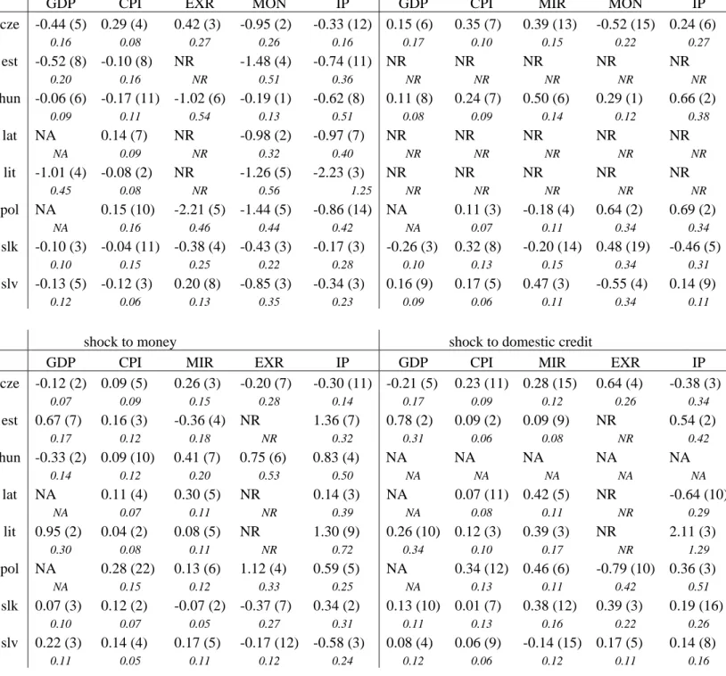
Table 1a: Peak impacts of monetary shocks

shock to interest rate shock to exchange rate

GDP CPI EXR MON IP GDP CPI MIR MON IP cze -0.44 (5) 0.29 (4) 0.42 (3) -0.95 (2) -0.33 (12) 0.15 (6) 0.35 (7) 0.39 (13) -0.52 (15) 0.24 (6) 0.16 0.08 0.27 0.26 0.16 0.17 0.10 0.15 0.22 0.27 est -0.52 (8) -0.10 (8) NR -1.48 (4) -0.74 (11) NR NR NR NR NR 0.20 0.16 NR 0.51 0.36 NR NR NR NR NR hun -0.06 (6) -0.17 (11) -1.02 (6) -0.19 (1) -0.62 (8) 0.11 (8) 0.24 (7) 0.50 (6) 0.29 (1) 0.66 (2) 0.09 0.11 0.54 0.13 0.51 0.08 0.09 0.14 0.12 0.38 lat NA 0.14 (7) NR -0.98 (2) -0.97 (7) NR NR NR NR NR NA 0.09 NR 0.32 0.40 NR NR NR NR NR lit -1.01 (4) -0.08 (2) NR -1.26 (5) -2.23 (3) NR NR NR NR NR 0.45 0.08 NR 0.56 1.25 NR NR NR NR NR pol NA 0.15 (10) -2.21 (5) -1.44 (5) -0.86 (14) NA 0.11 (3) -0.18 (4) 0.64 (2) 0.69 (2) NA 0.16 0.46 0.44 0.42 NA 0.07 0.11 0.34 0.34 slk -0.10 (3) -0.04 (11) -0.38 (4) -0.43 (3) -0.17 (3) -0.26 (3) 0.32 (8) -0.20 (14) 0.48 (19) -0.46 (5) 0.10 0.15 0.25 0.22 0.28 0.10 0.13 0.15 0.34 0.31 slv -0.13 (5) -0.12 (3) 0.20 (8) -0.85 (3) -0.34 (3) 0.16 (9) 0.17 (5) 0.47 (3) -0.55 (4) 0.14 (9) 0.12 0.06 0.13 0.35 0.23 0.09 0.06 0.11 0.34 0.11

shock to money shock to domestic credit

GDP CPI MIR EXR IP GDP CPI MIR EXR IP cze -0.12 (2) 0.09 (5) 0.26 (3) -0.20 (7) -0.30 (11) -0.21 (5) 0.23 (11) 0.28 (15) 0.64 (4) -0.38 (3) 0.07 0.09 0.15 0.28 0.14 0.17 0.09 0.12 0.26 0.34 est 0.67 (7) 0.16 (3) -0.36 (4) NR 1.36 (7) 0.78 (2) 0.09 (2) 0.09 (9) NR 0.54 (2) 0.17 0.12 0.18 NR 0.32 0.31 0.06 0.08 NR 0.42 hun -0.33 (2) 0.09 (10) 0.41 (7) 0.75 (6) 0.83 (4) NA NA NA NA NA 0.14 0.12 0.20 0.53 0.50 NA NA NA NA NA lat NA 0.11 (4) 0.30 (5) NR 0.14 (3) NA 0.07 (11) 0.42 (5) NR -0.64 (10) NA 0.07 0.11 NR 0.39 NA 0.08 0.11 NR 0.29 lit 0.95 (2) 0.04 (2) 0.08 (5) NR 1.30 (9) 0.26 (10) 0.12 (3) 0.39 (3) NR 2.11 (3) 0.30 0.08 0.11 NR 0.72 0.34 0.10 0.17 NR 1.29 pol NA 0.28 (22) 0.13 (6) 1.12 (4) 0.59 (5) NA 0.34 (12) 0.46 (6) -0.79 (10) 0.36 (3) NA 0.15 0.12 0.33 0.25 NA 0.13 0.11 0.42 0.51 slk 0.07 (3) 0.12 (2) -0.07 (2) -0.37 (7) 0.34 (2) 0.13 (10) 0.01 (7) 0.38 (12) 0.39 (3) 0.19 (16) 0.10 0.07 0.05 0.27 0.31 0.11 0.13 0.16 0.22 0.26 slv 0.22 (3) 0.14 (4) 0.17 (5) -0.17 (12) -0.58 (3) 0.08 (4) 0.06 (9) -0.14 (15) 0.17 (5) 0.14 (8) 0.11 0.05 0.11 0.12 0.24 0.12 0.06 0.12 0.11 0.16 Month of peaking in parentheses. Standard errors in italic. NA: non available, NR: non relevant.

(24)

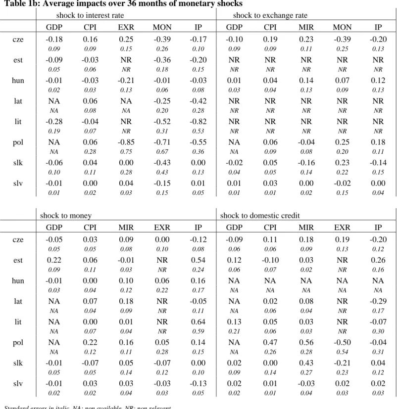
Table 1b: Average impacts over 36 months of monetary shocks

shock to interest rate shock to exchange rate GDP CPI EXR MON IP GDP CPI MIR MON IP cze -0.18 0.16 0.25 -0.39 -0.17 -0.10 0.19 0.23 -0.39 -0.20 0.09 0.09 0.15 0.26 0.10 0.09 0.09 0.11 0.25 0.13 est -0.09 -0.03 NR -0.36 -0.20 NR NR NR NR NR 0.05 0.06 NR 0.18 0.15 NR NR NR NR NR hun -0.01 -0.03 -0.21 -0.01 -0.03 0.01 0.04 0.14 0.07 0.12 0.02 0.03 0.13 0.06 0.08 0.03 0.04 0.13 0.09 0.13 lat NA 0.06 NA -0.25 -0.42 NR NR NR NR NR NA 0.08 NA 0.20 0.28 NR NR NR NR NR lit -0.28 -0.04 NR -0.52 -0.82 NR NR NR NR NR 0.19 0.07 NR 0.31 0.53 NR NR NR NR NR pol NA 0.06 -0.85 -0.71 -0.55 NA 0.06 -0.04 0.25 0.18 NA 0.28 0.75 0.67 0.36 NA 0.09 0.08 0.20 0.11 slk -0.06 0.04 0.00 -0.43 0.00 -0.02 0.05 -0.16 0.23 -0.14 0.10 0.11 0.28 0.43 0.13 0.04 0.05 0.14 0.22 0.15 slv -0.01 0.00 0.04 -0.15 0.01 0.01 0.03 0.00 -0.02 0.00 0.01 0.02 0.03 0.15 0.05 0.01 0.01 0.02 0.15 0.04

shock to money shock to domestic credit

GDP CPI MIR EXR IP GDP CPI MIR EXR IP cze -0.05 0.03 0.09 0.00 -0.12 -0.09 0.11 0.18 0.19 -0.20 0.05 0.05 0.08 0.10 0.08 0.06 0.06 0.09 0.13 0.12 est 0.22 0.06 -0.01 NR 0.54 0.12 -0.10 0.03 NR 0.26 0.09 0.11 0.03 NR 0.24 0.06 0.07 0.02 NR 0.16 hun -0.01 0.00 0.10 0.06 0.16 NA NA NA NA NA 0.03 0.04 0.12 0.22 0.17 NA NA NA NA NA lat NA 0.07 0.18 NR -0.05 NA 0.02 0.08 NR -0.29 NA 0.04 0.09 NR 0.11 NA 0.06 0.04 NR 0.17 lit NA 0.00 0.01 NR 0.64 0.13 0.05 0.03 NR -0.07 NA 0.07 0.04 NR 0.59 0.21 0.06 0.03 NR 0.30 pol NA 0.22 0.16 0.05 0.14 NA 0.47 0.56 -0.50 -0.04 NA 0.12 0.11 0.28 0.15 NA 0.26 0.28 0.54 0.31 slk -0.01 -0.07 0.05 -0.07 0.00 0.02 0.00 0.43 -0.21 0.04 0.05 0.05 0.14 0.12 0.10 0.09 0.14 0.27 0.23 0.12 slv -0.01 0.03 0.03 -0.03 -0.13 0.02 0.01 -0.03 0.02 0.02 0.02 0.02 0.04 0.03 0.05 0.02 0.01 0.04 0.03 0.03 Standard errors in italic. NA: non available, NR: non relevant.

(25)

Figures 1A: Czech Republic Response to a shock to the interest rate

-.8 -.6 -.4 -.2 .0 .2 5 10 15 20 25 30 35 Response of GDP -.2 -.1 .0 .1 .2 .3 .4 .5 5 10 15 20 25 30 35 Response of prices -0.4 0.0 0.4 0.8 1.2 5 10 15 20 25 30 35

Response of exchange rate

-1.6 -1.2 -0.8 -0.4 0.0 0.4 5 10 15 20 25 30 35 Response of money -.8 -.4 .0 .4 .8 5 10 15 20 25 30 35

Response of industrial production

-.1 .0 .1 .2 .3 .4 .5 5 10 15 20 25 30 35 Response of prices -0.4 0.0 0.4 0.8 5 10 15 20 25 30 35

-1.6 -1.2 -0.8 -0.4 0.0 0.4 5 10 15 20 25 30 35 Response of money

(26)

Figures 1B: Czech Republic Response to a shock to the exchange rate

-.6 -.4 -.2 .0 .2 .4 .6 5 10 15 20 25 30 35 Response of GDP -.2 -.1 .0 .1 .2 .3 .4 .5 .6 5 10 15 20 25 30 35 Response of prices -.4 -.2 .0 .2 .4 .6 .8 5 10 15 20 25 30 35

Response of interest rate

-1.0 -0.8 -0.6 -0.4 -0.2 0.0 0.2 0.4 5 10 15 20 25 30 35 Response of money -1.2 -0.8 -0.4 0.0 0.4 0.8 1.2 5 10 15 20 25 30 35

-.2 -.1 .0 .1 .2 .3 .4 .5 .6 .7 5 10 15 20 25 30 35 Response of prices -.4 -.2 .0 .2 .4 .6 .8 5 10 15 20 25 30 35

-1.2 -0.8 -0.4 0.0 0.4 0.8 5 10 15 20 25 30 35 Response of money

(27)

Figures 1C: Czech Republic

Response to a shock to the monetary aggregate

-.5 -.4 -.3 -.2 -.1 .0 .1 .2 .3 5 10 15 20 25 30 35 Response of GDP -.2 -.1 .0 .1 .2 .3 5 10 15 20 25 30 35 Response of prices -.2 -.1 .0 .1 .2 .3 .4 .5 .6 5 10 15 20 25 30 35

-.8 -.6 -.4 -.2 .0 .2 .4 .6 5 10 15 20 25 30 35

-1.2 -0.8 -0.4 0.0 0.4 0.8 5 10 15 20 25 30 35

-.2 -.1 .0 .1 .2 .3 .4 5 10 15 20 25 30 35 Response of prices -.2 -.1 .0 .1 .2 .3 .4 .5 .6 5 10 15 20 25 30 35

-.8 -.4 .0 .4

5 10 15 20 25 30 35

(28)

Figures 1D: Czech Republic

Response to a shock to the domestic credit aggregate

-.6 -.4 -.2 .0 .2 .4 5 10 15 20 25 30 35 Response of GDP -.2 -.1 .0 .1 .2 .3 .4 .5 5 10 15 20 25 30 35 Response of prices -.2 -.1 .0 .1 .2 .3 .4 .5 .6 .7 5 10 15 20 25 30 35

-0.8 -0.4 0.0 0.4 0.8 1.2 5 10 15 20 25 30 35

-1.2 -0.8 -0.4 0.0 0.4 0.8 5 10 15 20 25 30 35

-.2 -.1 .0 .1 .2 .3 .4 .5 .6 5 10 15 20 25 30 35 Response of prices -.2 -.1 .0 .1 .2 .3 .4 .5 .6 .7 5 10 15 20 25 30 35

-0.8 -0.4 0.0 0.4 0.8 1.2 1.6 2.0 5 10 15 20 25 30 35

(29)

Figures 2A: Estonia

Response to a shock to the interest rate

-1.2 -0.8 -0.4 0.0 0.4 0.8 1.2 5 10 15 20 25 30 35 Response of GDP -.5 -.4 -.3 -.2 -.1 .0 .1 .2 .3 5 10 15 20 25 30 35 Response of prices -3.0 -2.5 -2.0 -1.5 -1.0 -0.5 0.0 0.5 5 10 15 20 25 30 35 Response of money -1.5 -1.0 -0.5 0.0 0.5 1.0 1.5 5 10 15 20 25 30 35

-.8 -.6 -.4 -.2 .0 .2 .4 5 10 15 20 25 30 35 Response of prices -2.5 -2.0 -1.5 -1.0 -0.5 0.0 0.5 1.0 5 10 15 20 25 30 35 Response of money

(30)

Figures 2B: Estonia

-0.4 0.0 0.4 0.8 1.2 5 10 15 20 25 30 35 Response of GDP -.4 -.3 -.2 -.1 .0 .1 .2 .3 .4 .5 5 10 15 20 25 30 35 Response of prices -.8 -.6 -.4 -.2 .0 .2 .4 .6 5 10 15 20 25 30 35

-1.0 -0.5 0.0 0.5 1.0 1.5 2.0 2.5 5 10 15 20 25 30 35

-.6 -.4 -.2 .0 .2 .4 .6 5 10 15 20 25 30 35 Response of prices -.8 -.6 -.4 -.2 .0 .2 .4 5 10 15 20 25 30 35

(31)

Figures 2C: Estonia

-0.4 0.0 0.4 0.8 1.2 1.6 5 10 15 20 25 30 35 Response of GDP -.4 -.3 -.2 -.1 .0 .1 .2 .3 5 10 15 20 25 30 35 Response of prices -.4 -.3 -.2 -.1 .0 .1 .2 .3 5 10 15 20 25 30 35

-0.8 -0.4 0.0 0.4 0.8 1.2 1.6 5 10 15 20 25 30 35

-.5 -.4 -.3 -.2 -.1 .0 .1 .2 .3 5 10 15 20 25 30 35 Response of prices -.3 -.2 -.1 .0 .1 .2 .3 5 10 15 20 25 30 35

(32)

Figures 3A: Hungary

-.3 -.2 -.1 .0 .1 .2 .3 .4 5 10 15 20 25 30 35 Response of GDP -.4 -.3 -.2 -.1 .0 .1 .2 .3 5 10 15 20 25 30 35 Response of prices -2.5 -2.0 -1.5 -1.0 -0.5 0.0 0.5 1.0 5 10 15 20 25 30 35

-.6 -.4 -.2 .0 .2 .4 .6 5 10 15 20 25 30 35 Response of money -2.0 -1.5 -1.0 -0.5 0.0 0.5 1.0 5 10 15 20 25 30 35

-.3 -.2 -.1 .0 .1 .2 .3 .4 5 10 15 20 25 30 35 Response of prices -1.2 -0.8 -0.4 0.0 0.4 0.8 5 10 15 20 25 30 35

-.5 -.4 -.3 -.2 -.1 .0 .1 .2 .3 .4 5 10 15 20 25 30 35 Response of money

(33)

Figures 3B: Hungary

Response to a shock to the exchange rate

-.6 -.4 -.2 .0 .2 .4 5 10 15 20 25 30 35 Response of GDP -.4 -.3 -.2 -.1 .0 .1 .2 .3 .4 .5 5 10 15 20 25 30 35 Response of prices -0.4 0.0 0.4 0.8 5 10 15 20 25 30 35

-.3 -.2 -.1 .0 .1 .2 .3 .4 .5 .6 5 10 15 20 25 30 35 Response of M2 -0.8 -0.4 0.0 0.4 0.8 1.2 1.6 5 10 15 20 25 30 35 -.2 -.1 .0 .1 .2 .3 .4 5 10 15 20 25 30 35 Response of prices -.3 -.2 -.1 .0 .1 .2 .3 .4 .5 5 10 15 20 25 30 35

-.2 -.1 .0 .1 .2 .3 .4 .5 5 10 15 20 25 30 35 Response of M2 Response of industrial production

(34)

Figures 3C Hungary

-.8 -.6 -.4 -.2 .0 .2 .4 5 10 15 20 25 30 35 Response of GDP -.3 -.2 -.1 .0 .1 .2 .3 .4 5 10 15 20 25 30 35 Response of prices -0.4 -0.2 0.0 0.2 0.4 0.6 0.8 1.0 5 10 15 20 25 30 35

-1.5 -1.0 -0.5 0.0 0.5 1.0 1.5 2.0 5 10 15 20 25 30 35

-.3 -.2 -.1 .0 .1 .2 .3 .4 .5 .6 5 10 15 20 25 30 35 Response of prices -.4 -.2 .0 .2 .4 .6 .8 5 10 15 20 25 30 35

-0.8 -0.4 0.0 0.4 0.8 1.2 1.6 5 10 15 20 25 30 35

(35)

Figures 4A Latvia Figures 4B Latvia Figures 4C Latvia

Response to a shock to the Response to a shock to the Response to a shock to the

interest rate monetary aggregate domestic credit aggregate

-2.0 -1.6 -1.2 -0.8 -0.4 0.0 0.4 0.8 5 10 15 20 25 30 35 Response of industrial production

-.2 -.1 .0 .1 .2 .3 .4 5 10 15 20 25 30 35 Response of prices -2.0 -1.6 -1.2 -0.8 -0.4 0.0 0.4 0.8 5 10 15 20 25 30 35 Response of money -1.0 -0.5 0.0 0.5 1.0 5 10 15 20 25 30 35

-.2 -.1 .0 .1 .2 .3 5 10 15 20 25 30 35 Response of prices -.8 -.6 -.4 -.2 .0 .2 .4 .6 5 10 15 20 25 30 35

-1.6 -1.2 -0.8 -0.4 0.0 0.4 0.8 5 10 15 20 25 30 35

-.2 -.1 .0 .1 .2 .3 5 10 15 20 25 30 35 Response of prices -.4 -.2 .0 .2 .4 .6 .8 5 10 15 20 25 30 35

(36)

Figures 5A Lithuania

-2.0 -1.6 -1.2 -0.8 -0.4 0.0 0.4 5 10 15 20 25 30 35 Response of GDP -.4 -.3 -.2 -.1 .0 .1 .2 5 10 15 20 25 30 35 Response of prices -2.5 -2.0 -1.5 -1.0 -0.5 0.0 0.5 5 10 15 20 25 30 35 Response of money -5 -4 -3 -2 -1 0 1 2 5 10 15 20 25 30 35

-.4 -.3 -.2 -.1 .0 .1 .2 .3 .4 5 10 15 20 25 30 35 Response of prices -3 -2 -1 0 1 2 5 10 15 20 25 30 35 Response of money

(37)

Figures 5B Lithuania

-0.8 -0.4 0.0 0.4 0.8 1.2 1.6 5 10 15 20 25 30 35 Response of GDP -.3 -.2 -.1 .0 .1 .2 .3 5 10 15 20 25 30 35 Response of prices -.5 -.4 -.3 -.2 -.1 .0 .1 .2 .3 .4 5 10 15 20 25 30 35

-4 -3 -2 -1 0 1 2 3 4 5 10 15 20 25 30 35

-.6 -.4 -.2 .0 .2 .4 .6 5 10 15 20 25 30 35 Response of prices -.5 -.4 -.3 -.2 -.1 .0 .1 .2 .3 .4 5 10 15 20 25 30 35

(38)

Figures 5C Lithuania

-1.2 -0.8 -0.4 0.0 0.4 0.8 1.2 5 10 15 20 25 30 35 Response of GDP -.2 -.1 .0 .1 .2 .3 .4 5 10 15 20 25 30 35 Response of prices -.4 -.2 .0 .2 .4 .6 .8 5 10 15 20 25 30 35

-4 -3 -2 -1 0 1 2 3 4 5 5 10 15 20 25 30 35

-.4 -.2 .0 .2 .4 .6 5 10 15 20 25 30 35 Response of prices -.4 -.2 .0 .2 .4 .6 .8 5 10 15 20 25 30 35

(39)

Figures 6A: Poland

-2.0 -1.5 -1.0 -0.5 0.0 0.5 1.0 1.5 5 10 15 20 25 30 35

-1.0 -0.5 0.0 0.5 1.0 5 10 15 20 25 30 35 Response of prices -4 -3 -2 -1 0 1 2 3 5 10 15 20 25 30 35

-3 -2 -1 0 1 2 5 10 15 20 25 30 35 Response of money

(40)

Figures 6B: Poland

-0.8 -0.4 0.0 0.4 0.8 1.2 1.6 5 10 15 20 25 30 35

-.2 -.1 .0 .1 .2 .3 .4 5 10 15 20 25 30 35 Response of prices -.5 -.4 -.3 -.2 -.1 .0 .1 .2 .3 .4 5 10 15 20 25 30 35

-0.8 -0.4 0.0 0.4 0.8 1.2 1.6 5 10 15 20 25 30 35 Response of money

(41)

Figures 6C: Poland

-0.8 -0.4 0.0 0.4 0.8 1.2 5 10 15 20 25 30 35

-.2 -.1 .0 .1 .2 .3 .4 .5 .6 .7 5 10 15 20 25 30 35 Response of prices -.4 -.2 .0 .2 .4 .6 .8 5 10 15 20 25 30 35

-1.5 -1.0 -0.5 0.0 0.5 1.0 1.5 2.0 5 10 15 20 25 30 35

(42)

Figures 6D: Poland

-1.5 -1.0 -0.5 0.0 0.5 1.0 1.5 5 10 15 20 25 30 35

-0.8 -0.4 0.0 0.4 0.8 1.2 1.6 2.0 2.4 5 10 15 20 25 30 35 Response of prices -1.0 -0.5 0.0 0.5 1.0 1.5 2.0 2.5 5 10 15 20 25 30 35

-3 -2 -1 0 1 2 5 10 15 20 25 30 35

(43)

Figures 7A: Slovak Republic Response to a shock to the interest rate

-.4 -.3 -.2 -.1 .0 .1 .2 5 10 15 20 25 30 35 Response of GDP -.4 -.3 -.2 -.1 .0 .1 .2 .3 .4 5 10 15 20 25 30 35 Response of prices -1.0 -0.5 0.0 0.5 1.0 5 10 15 20 25 30 35

-2.0 -1.5 -1.0 -0.5 0.0 0.5 1.0 5 10 15 20 25 30 35 Response of money -.8 -.6 -.4 -.2 .0 .2 .4 .6 5 10 15 20 25 30 35

-.4 -.3 -.2 -.1 .0 .1 .2 .3 .4 5 10 15 20 25 30 35 Response of prices -1.2 -0.8 -0.4 0.0 0.4 0.8 5 10 15 20 25 30 35

-1.2 -0.8 -0.4 0.0 0.4 0.8 5 10 15 20 25 30 35 Response of money

(44)

Figures 7B: Slovak Republic Response to a shock to the exchange rate

-.5 -.4 -.3 -.2 -.1 .0 .1 .2 5 10 15 20 25 30 35 Response of GDP -.3 -.2 -.1 .0 .1 .2 .3 .4 .5 .6 5 10 15 20 25 30 35 Response of prices -.6 -.5 -.4 -.3 -.2 -.1 .0 .1 .2 .3 5 10 15 20 25 30 35

-1.2 -0.8 -0.4 0.0 0.4 0.8 1.2 5 10 15 20 25 30 35 Response of money -1.2 -0.8 -0.4 0.0 0.4 0.8 5 10 15 20 25 30 35

-.4 -.2 .0 .2 .4 .6 .8 5 10 15 20 25 30 35 Response of prices -.5 -.4 -.3 -.2 -.1 .0 .1 .2 .3 5 10 15 20 25 30 35

-0.8 -0.4 0.0 0.4 0.8 1.2 1.6 5 10 15 20 25 30 35 Response of money

(45)

Figures 7C Slovak Republic

-.3 -.2 -.1 .0 .1 .2 .3 5 10 15 20 25 30 35 Response of GDP -.5 -.4 -.3 -.2 -.1 .0 .1 .2 .3 5 10 15 20 25 30 35 Response of prices -.4 -.3 -.2 -.1 .0 .1 .2 .3 .4 .5 5 10 15 20 25 30 35

-.8 -.4 .0 .4

5 10 15 20 25 30 35

-0.8 -0.4 0.0 0.4 0.8 1.2 5 10 15 20 25 30 35

-.4 -.3 -.2 -.1 .0 .1 .2 .3 5 10 15 20 25 30 35 Response of prices -.3 -.2 -.1 .0 .1 .2 .3 5 10 15 20 25 30 35

-1.2 -0.8 -0.4 0.0 0.4 0.8 5 10 15 20 25 30 35

(46)

Figures 7d: Slovak Republic

-.4 -.3 -.2 -.1 .0 .1 .2 .3 .4 5 10 15 20 25 30 35 -.6 -.4 -.2 .0 .2 .4 .6 .8 5 10 15 20 25 30 35 Response of prices -1.0 -0.5 0.0 0.5 1.0 1.5 2.0 5 10 15 20 25 30 35

-1.5 -1.0 -0.5 0.0 0.5 1.0 5 10 15 20 25 30 35

Response of exchange rate Response of GDP -1.2 -0.8 -0.4 0.0 0.4 0.8 5 10 15 20 25 30 35

-.6 -.4 -.2 .0 .2 .4 5 10 15 20 25 30 35 Response of prices -.2 -.1 .0 .1 .2 .3 .4 5 10 15 20 25 30 35

-2.0 -1.5 -1.0 -0.5 0.0 0.5 1.0 5 10 15 20 25 30 35

(47)

Figures 8A: Slovenia

-.4 -.3 -.2 -.1 .0 .1 .2 5 10 15 20 25 30 35 Response of GDP -.3 -.2 -.1 .0 .1 .2 5 10 15 20 25 30 35 Response of prices -.3 -.2 -.1 .0 .1 .2 .3 .4 .5 5 10 15 20 25 30 35

-2.0 -1.6 -1.2 -0.8 -0.4 0.0 0.4 5 10 15 20 25 30 35 Response of money -.8 -.4 .0 .4 5 10 15 20 25 30 35 -.3 -.2 -.1 .0 .1 .2 5 10 15 20 25 30 35 Response of prices -.3 -.2 -.1 .0 .1 .2 .3 .4 .5 .6 5 10 15 20 25 30 35

-2.0 -1.6 -1.2 -0.8 -0.4 0.0 0.4 5 10 15 20 25 30 35 Response of money Response of industrial production

(48)

Figures 8B: Slovenia

-.4 -.3 -.2 -.1 .0 .1 .2 .3 .4 5 10 15 20 25 30 35 Response of GDP -.2 -.1 .0 .1 .2 .3 5 10 15 20 25 30 35 Response of prices -.6 -.4 -.2 .0 .2 .4 .6 .8 5 10 15 20 25 30 35

-1.6 -1.2 -0.8 -0.4 0.0 0.4 0.8 5 10 15 20 25 30 35 Response of money -.6 -.4 -.2 .0 .2 .4 .6 5 10 15 20 25 30 35

-.2 -.1 .0 .1 .2 .3 .4 5 10 15 20 25 30 35 Response of prices -.6 -.4 -.2 .0 .2 .4 .6 .8 5 10 15 20 25 30 35

-1.6 -1.2 -0.8 -0.4 0.0 0.4 0.8 1.2 5 10 15 20 25 30 35 Response of money

(49)

Figures 8C: Slovenia

-.4 -.3 -.2 -.1 .0 .1 .2 .3 .4 .5 5 10 15 20 25 30 35 Response of GDP -.1 .0 .1 .2 .3 5 10 15 20 25 30 35 Response of prices -.4 -.3 -.2 -.1 .0 .1 .2 .3 .4 .5 5 10 15 20 25 30 35

-.5 -.4 -.3 -.2 -.1 .0 .1 .2 .3 .4 5 10 15 20 25 30 35

-1.2 -0.8 -0.4 0.0 0.4 5 10 15 20 25 30 35

-.10 -.05 .00 .05 .10 .15 .20 .25 5 10 15 20 25 30 35 Response of prices -.4 -.3 -.2 -.1 .0 .1 .2 .3 .4 5 10 15 20 25 30 35

-.4 -.3 -.2 -.1 .0 .1 .2 5 10 15 20 25 30 35

(50)

-.2 -.1 .0 .1 .2 .3 .4 5 10 15 20 25 30 35 Response of GDP -.2 -.1 .0 .1 .2 5 10 15 20 25 30 35 Response of prices -.4 -.3 -.2 -.1 .0 .1 .2 .3 5 10 15 20 25 30 35

-.3 -.2 -.1 .0 .1 .2 .3 .4 5 10 15 20 25 30 35

-.8 -.4 .0 .4 .8 5 10 15 20 25 30 35

-.2 -.1 .0 .1 .2 5 10 15 20 25 30 35 Response of prices -.5 -.4 -.3 -.2 -.1 .0 .1 .2 .3 .4 5 10 15 20 25 30 35

-.5 -.4 -.3 -.2 -.1 .0 .1 .2 .3 .4 5 10 15 20 25 30 35

Figures 8D: Slovenia