The optimal carbon sequestration in agricultural soils: does the dynamics of the physical process matter?

HAL Id: halshs-00115685

https://halshs.archives-ouvertes.fr/halshs-00115685

Submitted on 22 Nov 2006

HAL is a multi-disciplinary open access archive for the deposit and dissemination of sci-entific research documents, whether they are pub-lished or not. The documents may come from teaching and research institutions in France or

L’archive ouverte pluridisciplinaire HAL, est destinée au dépôt et à la diffusion de documents scientifiques de niveau recherche, publiés ou non, émanant des établissements d’enseignement et de recherche français ou étrangers, des laboratoires

The optimal carbon sequestration in agricultural soils:

does the dynamics of the physical process matter?

Lionel Ragot, Katheline Schubert

To cite this version:

Lionel Ragot, Katheline Schubert. The optimal carbon sequestration in agricultural soils: does the dynamics of the physical process matter?. 2006. �halshs-00115685�

Maison des Sciences Économiques, 106-112 boulevard de L'Hôpital, 75647 Paris Cedex 13

http://mse.univ-paris1.fr/Publicat.htm

Centre d’Economie de la Sorbonne

UMR 8174

The optimal carbon sequestration in agricultural soils!:

does the dynamics of the physical process matter!?

Lionel RAGOT

Katheline SCHUBERT

The optimal carbon sequestration in agricultural soils:

does the dynamics of the physical process matter?

Lionel Ragota;b and Katheline Schuberta

a _CES

, Université de Paris 1

b _{MÉDEE, Université de Lille 1}

13th March 2006

The authors acknowledge …nancial support from the French Ministry of Ecology and Sustainable Development (APR GICC 2002). The usual disclaimers apply.

Résumé

Le Protocole de Kyoto, entré en vigueur en février 2005, autorise les pays signataires à recourir à des “activités supplémentaires” permettant en particulier la séquestration de carbone dans les sols. Les travaux existants qui étudient la sequestration optimale de carbone reconnaissent l’importance du processus temporel de séquestration, mais négligent le fait que ce processus est dissymétrique. Ce papier prend en compte explicitement la dynamique de la séquestration. Sa première contribution est technique : nous résolvons un problème de contrôle optimal à deux phases et processus dynamique dis-symétrique. Sa seconde contribution est empirique : nous montrons que l’erreur commise en supposant la séquestration immédiate peut être très signi…cative, et simulons le sentier optimal de séquestration / déséquestration pour des fonctions de béné…ce, de dommage et de coût particulières.

Codes JEL : C61, H23, Q01, Q15

Mots clés : environnement, agriculture, séquestration de carbone, Protocole de Kyoto, contrôle optimal.

Abstract

The Kyoto Protocol, which came in force in February 2005, allows countries to resort to “sup-plementary activities” consisting particularly in carbon sequestration in agricultural soils. Existing papers studying the optimal carbon sequestration recognize the importance of the temporality of sequestration, but overlook the fact that it is a dissymmetric dynamic process. This paper takes ex-plicitely into account the temporality of sequestration. Its …rst contribution is technical: we solve an optimal control problem with two stages and a dissymmetric dynamic process. The second contribu-tion is empirical: we show that the error made when sequestracontribu-tion is supposed immediate can be very signi…cant, and we exhibit numerically the optimal path of sequestation / de-sequestration for speci…c bene…t, damage and cost functions, and a calibration that mimics roughly the world conditions.

JEL Classi…cation: C61, H23, Q01, Q15

1

Introduction

The Kyoto Protocol, rati…ed by the European countries in 2002 and in force from February 2005, allows countries to resort to “supplementary activities” consisting in the sequestration of carbon in forests and in agricultural soils (Articles 3.3 and 3.4). The emissions trapped by such volontary activities, set up after 1990, can be deduced from the emissions of greenhouse gas. They can be the result of a¤orestation projects (Article 3.3) or of changes of practices in the agricultural and forestry sectors (Article 3.4). As far as this last article is concerned, the list of eligible activities proposed by the IPCC gives appreciable opportunities of reduction of emissions to countries possessing signi…cant surfaces of agricultural land. For example, gross French emissions of greenhouse gas were estimated at 148 MtC in 2000. France emits low levels of GHG per capita and will encounter di¢ culties in further reducing its emissions, in part because of the importance of French nuclear energy generating capacity. Given the area of land devoted to agriculture, the prospects opened by Article 3.4 may be of interest for the French policy of greenhouse gas mitigation. The French National Institute for Agricultural Research has recently estimated the potential additional carbon storage for the next 20 years, between 1 and 3 MtC/year, for the whole of mainland France (INRA (2002)). This potential is equivalent to 1 to 2% of annual French greenhouse gas emissions, a large proportion of the e¤orts required to comply with the commitments to the Kyoto Protocol. At the European level, this potential is estimated at 1.5 to 1.7% of the EU-15 anthropogenic CO2 emissions during the …rst commitment period (European

Climate Change Program (2003)).

The Bonn Agreement (COP6bis) in July 2001 clari…es the implementation of Article 3.4: eligible activities in agriculture comprise “cropland management”, “grazing land management” and “reve-getation”, provided that these activities have occured since 1990 and are human-induced. Carbon sequestration can occur either through a reduction in soil disturbance (zero tillage or reduced tillage, set-aside land, growth of perennial crops...) or through an increase of the carbon input to the soil (animal manure, sewage sludge, compost...). Switching from conventional arable agriculture to other land-uses with higher carbon input or reduced disturbance can also increase the soil carbon stock (conversion of arable land to grassland or woodland, organic farming...).

Lal et al. (1998) provide estimates of the carbon sequestration potential of agricultural manage-ment options in the USA. A few studies present estimations of agricultural soil carbon sequestration potentials for EU-15 (see European Climate Change Programme (2003)), and one study does the same for France (INRA (2002)). They all show that soil carbon sequestration is a non-linear process. Increases in soil carbon are often greatest soon after a land use or land management change is im-plemented. There is also a sink saturation e¤ect: as the soil reaches a new equilibrium, the rate of change decreases, so that after 20 to 100 years a new equilibrium is reached and no further change takes place. Moreover, by changing agricultural management or land-use, soil carbon is lost more rapidly than it accumulates (Smith et al. (1996), INRA (2002)). Carbon de-sequestation is far faster than sequestration or, to put it di¤erently, carbon storage in agricultural soils takes far more time than carbon release (the unit of measure of the storage time is tens of years, the one of release is years, see INRA (2002)).

The aim of this paper is to study the optimal policy of carbon sequestration in agricultural soils. While many technical papers try to quantify the potential of carbon sequestration, there are very few papers studying the optimal path of carbon sequestration. To the best of our knowledge, the paper by Feng, Zhao and Kling (2002) is the only one. But their dynamic representation of the process is limited by the assumption that the sequestration potential of a unit of land on which a change in land use or land management takes place is instantaneously obtained. Technical papers recognize the importance of the temporality of sequestration, and we take in this paper this temporality explicitely into account. Moreover, we also take into account the fact that sequestration is a dissymmetric dynamic process, which most experts in the …eld of agriculture consider determining (INRA (2002)). Anyhow, the question is: what should the dissymmetry of the process be important at all? The answer to this question is obvious in a decentralized framework, where agents can be incited to sequester carbon by an appropriate policy, and then be incited to stop using the sequestering practices if the policy is not permanent. In the case of the optimal policy that we study here, temporary sequestration could be optimal if the terms of the trade-o¤ between emissions abatement and carbon sequestration in order to reduce the stock of carbon in the atmosphere change in the course of time. These terms could change because of a technical progress enhancing the possibilities of abatement, or because of the characteristics of the dynamic process of sequestration / de-sequestration. We focus here on the second possibility.

We adapt the Feng, Zhao and Kling’s (2002) model to take into account explicitly the dynamics of the sequestration process. The main characteristics of the model are the following. The economic activity causes carbon emissions that accumulate in the atmosphere. Bene…ts are associated to this emissions – or, equivalently, emissions reduction is costly –, and damages to the atmospheric carbon stock. Sequestration has a cost, depending on how much land is devoted to it. When a change of practice occurs on a unit of land in order to enhance its carbon sequestration, it stores its potential gradually; when the unit of land returns to the usual practice, it releases carbon more rapidly than it has stored it. The total amount of land on which a change of practice can take place is bounded from above. In the same way, at each date, the amount of new land that can be used to store carbon is bounded from above, as well as the amount of land that can go back to the usual practice. This assumption expresses in a simple way the existence of adjustment costs and of physical limits to the land-use changes. The sequestration / de-sequestration process is supposed irreversible, in the sense that it is impossible to sequester again on a unit of land that has already been used for sequestration and then went back to the usual practice. The problem is then to …nd at each date the optimal carbon emissions and the amount of land newly devoted to sequestration or de-sequestration, subject to the evolution of the carbon and land stocks and of the constraints. We characterize analytically the di¤erent possible solutions. Then, we calibrate the model and make numerical simulations that allow us to compare our solutions to the ones obtained when the dynamics and the dissymmetry of the process are not taken into account.

Section 2 presents the modelling of the sequestration / de-sequestration process. Section 3 is devoted to the exposition and the analytical resolution of the dynamic optimization problem taking the temporality and the dissymmetry of this process into consideration. In section 4, numerical simulations

allow us to exhibit the optimal path of carbon sequestration, for speci…c bene…t of emissions, damage and cost of sequestration functions, and to compare it with the path obtained when sequestration and de-sequestration are taken to be immediate. Section 5 concludes.

2

The dynamics of carbon sequestration in agricultural soils

The total amount of agricultural land is supposed to be B; constant over time and exogenous. Land is homogeneous and produces a unique agricultural good. The di¤erent units of land may however di¤er according to the agricultural practices used on them. Two types of practices are distinguished: the “usual” practice and a “sequestering” practice, allowing land to store more carbon. All units of land are supposed to be initially cultivated with the usual practice.

Physical studies clearly show that additional sequestration is a non-linear process: it is high in the …rst years following the change of practice, then decreases and tends towards zero as the new equilibrium is approached. We adopt here, following the results of Hénin and Dupuis (1945), an exponential approximation of the sequestration process.

The maximal amount of carbon that can be stored in a unit of land’s soil is cs . Let cs(t; z) represent the amount of carbon in the soil at date t for a change of practice taking place at date z, and cs0 the amount of carbon stored with the usual practice (cs > cs0 0). The dynamics of

sequestration in a unit of land is then

cs(t; z) = cs + (csn cs )e s(t z); t z; (1)

where s > 0 is the parameter of speed of the sequestration process.

Let us now consider a unit of land returning to the usual practice at date & after having experienced the …rst change of practice at date z. cs(&; z) is the amount of carbon that the sequestering practice has allowed the land to store until date &, and cs(t; &; z) the amount of carbon remaining in the soil at date t: We have cs(t; &; z) = csn+ (cs(&; z) csn)e s 0_{(t &)} ; t & z = csn+ (cs csn)(1 e s(& z))e s 0_{(t &)} ; t & z; (2)

where s0 > 0 is the parameter of speed of the de-sequestration process. The assumption s0 > s will allow us to take into account the fact that the storage process is slower than the release process.

Let us assume …rst that the only possible change of practice is from the usual to a sequestering one (no possibility of return to the usual practice). The aggregate carbon stock stored in agricultural soils at t is then de…ned by

CS(t) = csnB + Z t 0 a(z)(cs(t; z) csn)dz = csnB + (cs csn) Z t 0 a(z)(1 e s(t z))dz; (3)

where a(z) is the number of units of land that moved from the usual practice to a sequestering one at date z. Feng et al. (2002) suppose that because of various technical and economic constraints, the

number of units of land on which a change of practice can take place at each date is bounded from above: a(z) _{a 8z. To avoid unessential technical di¢ culties (see footnote 2), we make the stronger} assumption that a is a discrete variable that can only take the two values 0 and a: the number of units of land on which the practice can change is either nil or maximum.

The fact that the change of practice can take place at di¤erent dates on di¤erent units of land introduces an heterogeneity among the units, even if land is initially homogeneous. At date t; all the units which have adopted a sequestering practice do not necessarily store the same amount of carbon, the amount stored by each of them depending on the date of the change of practice.

Let us suppose now that a sequence usual practice / sequestering practice / usual practice is possible. There exist for a given unit of land three conceivable con…gurations1 at date t:

either it has been cultivated with the usual practice from the beginning, and the carbon stored is csn ;

or it has experienced a single change of practice at date z < t, and the carbon stored is cs(t; z) given by equation (1);

or it has experienced the two changes of practice, respectively at dates z and & with z < & < t; and the carbon stored is cs(t; &; z) given by equation (2).

The calculation of the aggregate carbon stock is complicated because of the heterogeneity due to the timing of sequestration. Nevertheless, in the case of the social optimum and under the assumption of homogeneity of the land, the units of land which must come back to the usual practice are necessarily those which have changed practice last (last in – …rst out principle). The bene…t of a return to the usual practice on a given unit of land is indeed independant of the carbon stored in its soil. Besides, the social damage due to this return is all the smaller since this carbon stock is low, which corresponds to the last unit having changed practice. The aggregate stock then writes

CS(t) = csnB + Z T0 0 a(z)(cs(t; z) csn)dz Z t T0 b(z)rs(t; z)dz;

with T0 the date at which the carbon release begins and rs(t; z) the “virtual release” at date t in the b(z) units of lands that went back to the usual practice at date z (cf. …gure 1). Sequestration begins in a given unit of land at date (z) and stops at date z: The amount of carbon stored in the soil of this unit at this date is cs(z; (z)). The amount of carbon stored at date t is cs(t; z; (z)): If the sequestering practice had continued until date t the sequestration would have been equal to cs(t; (z)): The di¤erence between this virtual storage and the real one is rs(t; z): We then have

rs(t; z) = cs(t; (z)) cs(t; z; (z))

= (cs csn) (1 e s(t (z))) (1 e s(z (z)))e s

0_{(t z)}

:

-6 cs (z) cs(z; (z)) cs(t; (z)) cs(t; z; (z)) z t rs(t; z)

Figure 1: Carbon storage and release

The last in – …rst out principle allows us to de…ne (z) by Z T0 (z) a( )d = Z z T0 b( )d :

For the same reasons than in the case of a(t); we make the assumption that the number of units of land that can go back to the usual practice at each date is either 0 or a: b(t) = f0; ag 8t.

The aggregate carbon stock sequestered in agricultural soils is …nally: 8 > > < > > : CS(t) = csnB + (cs csn) Rt 0 a(z)(1 e s(t z))dz 8t T0 CS(t) = csnB + (cs csn) RT0 0 a(z)(1 e s(t z))dz (cs csn) Rt T0b(z) (1 e s(t (z))) (1 e s(z (z)))e s 0_{(t z)} dz _{8t > T}0; (4)

and the corresponding ‡ow of carbon emissions trapped at each date in the soils is: 8 > > < > > : F (t) = (cs csn)sR₀ta(z)e s(t z)dz 8t T0 F (t) = (cs csn)sRT 0 0 a(z)e s(t z)_dz (cs csn)R_Tt0b(z) se s(t (z))+ s0(1 e s(z (z)))e s 0_{(t z)} dz _{8t > T}0: (5)

Finally, the stock of agricultural land cultivated with the sequestering practice at date t is: (

A(t) =R₀ta(z)dz _8t T0

A(t) =R₀T0a(z)dz R_Tt₀b(z)dz _{8t > T}0 (6) with 0 A(t) _{B; a(t) = f0; ag and b(t) = f0; ag 8t}

3

The optimal solution

3.1 The social planner’s program

The social planner maximizes the total surplus associated to the emissions of carbon by the economic activity, composed of the di¤erence between the bene…ts of emissions and the sum of the costs of carbon sequestration in agricultural soils and of the damage of climate change.

The carbon stock in the atmosphere is subject to a natural assimilation process at the constant rate > 0; besides, it is augmented by net emissions, equal to raw emissions E(t) minus emissions removed

from the atmosphere by sequestration in agricultural soils F (t). The equation of accumulation of the carbon stock is then

_

S(t) = S(t) + E(t) F (t); (7)

where F (t) is given by equation (5).

The initial carbon stock is given, S(0) = S0 > 0.

The bene…ts of emissions are B(E(t)); with B0(E(t)) > 0 and B00(E(t)) 0:

The damage function is D(S(t)); with D0(S(t)) > 0: We do not make any a priori assumption on D00(S(t)): the marginal damage can be decreasing, constant or increasing.

The cost of sequestration is C(A(t)); with C0_{(A(t)) > 0 and C}00_{(A(t)) > 0: This cost is an}

oppor-tunity cost and also a cost associated to the new equipment that the change of practice requires. The social discount rate is r; supposed constant.

The date at which carbon release begins to take place is T0_:

The social planner seeks to maximize (with_{ec = cs} csn)

max V = Z ₁ 0 e rt(B(E(t) D(S(t)) C(A(t)))dt; subject to 8 > > > > > > > > > > > > > > < > > > > > > > > > > > > > > : _ S(t) = S(t) + E(t) F (t) _ A(t) = a(t) b(t) 8 > > < > > : F (t) =_ecsR₀ta(z)e s(t z)dz _8t T0 F (t) =_ecsR₀T0a(z)e s(t z)dz ecRTt0b(z) se s(t (z))+ s0(1 e s(z (z)))e s 0_{(t z)} dz _{8t > T}0 RT0 (z)a( )d = Rz T0b( )d

0 A(t) _{B, a(t) = f0; ag and b(t) = f0; ag 8t} S(0) = S0 and A(0) = 0 given.

The ‡ow of carbon stored in agricultural soils at instant t; F (t); is determined di¤erently depending on the relevant stage: carbon storage (before T0) or carbon release (after T0). The problem is then a two-stage optimal control problem. In order to solve it, we adapt to our case the method proposed by Tomiyama (1985), Tomiyama and Rossana (1989) and Saglam (2002) for this type of problems. The derivation of the …rst order necessary conditions of optimality and of the matching conditions in the general case is left to Appendix A.

3.2 Before T0_{: sequestration}

The social planner solves an optimization program in …nite horizon, considering that the horizon T0 and the value function of the program after T0 V+(S(T0); A(T0)) are given. By de…nition of T0; we

have b(t) = 0 8t T0_{: The social planner’s program then writes} 8 > > > > > > > < > > > > > > > :

maxR₀T0e rt(B(E(t)) D(S(t)) C(A(t)))dt + V+(S(T0); A(T0))

_

S(t) = S(t) + E(t) _ecsR₀ta(z)e s(t z)dz _

A(t) = a(t)

0 A(t) _{B and a(t) = f0; ag 8t} S(0) = S0, A(0) = 0 given.

(8)

We note 1 the shadow price of the carbon stock S and 2 the one of the land used for

sequest-ration A. The current value Hamiltonian of this program is then (see Appendix A):

H = e rt(B(E(t)) D(S(t)) C(A(t))) + 1 (t) ( S(t) + E(t)) + 2 (t)a(t)

ecsa(t) Z T0

t

1 (z)e s(z t)dz: (9)

First of all, the Hamiltonian is linear in the control variable a(t): The coe¢ cient associated to a(t) in the Hamiltonian is

(t) = 2 (t) ecs

Z T0

t

1 (z)e s(z t)dz: (10)

It represents the di¤erence between the marginal bene…t of sequestration and its marginal cost. The marginal bene…t is the sum of the ‡ows of carbon sequestered until T0 _{by an additional unit of}

land devoted to sequestration at t; evaluated at the (negative) shadow value of the carbon stock 1 .

The marginal cost is the (negative) shadow price of the land used for sequestration 2 : As long as

this coe¢ cient (t) is positive, the bene…t of sequestration is greater than its cost and a(t) = a; when the coe¢ cient becomes negative, a(t) = 02. It may happen that sequestration stops while (t) is still positive, if all the lands suitable for sequestration are already used. The date T at which sequestration stops can then be:

T1 in the case of a corner solution, with A(T1) = B and (T1) > 0;

T2 in the case of an interior solution, with A(T2) < B and (T2) = 0:

Besides, between 0 and T (equal to T1 or T2) we have _A(t) = a, which implies

A(t) = (

at; t T

A(T ) = aT; t_{2 [T; T}0_{] :} (11)

The …rst order necessary conditions are (see Appendix A): @H @E(t) = 0 , e rt_B0_{(E(t)) +} 1 (t) = 0; (12) @H @S(t) + _1 (t) = 0 , e rt_D0_(S(t)) 1 (t) + _1 (t) = 0; (13) @H @A(t)+ _2 (t) = 0 , e rt_C0_{(A(t)) + _} 2 (t) = 0: (14) 2

Without the assumption that a(t) is a discrete variable, we could have had (t) = 0 for an interval of values of t; that could not have been reduced to the single value T: Feng et al. (2002) obtain this kind of solution. This would have been untractable in our problem.

Equations (12) and (13) allow us to obtain the growth rate of emissions: _ E(t) E(t) = B0_(E(t)) E(t)B00_(E(t)) D0_(S(t)) B0_(E(t)) (r + ) : (15)

Besides, the equation of accumulation of the carbon stock is

_ S(t) = S(t) + E(t) F (t); (16) with F (t) =_eca ( 1 e st ; 0 t T e st esT 1 ; T t T0: (17)

These two dynamic equations allow us to obtain E(t) and S(t) 8t 2 [0; T0] ; as functions of E(0) and T which are still unknown.

Using equation (11), equation (14) integrates into:

2 (t) = ( 2 (0) + Rt 0e rzC0(A(z))dz; 0 t T; 2 (T ) C 0_{(A(T ))} r e rt _e rT _{; T t T}0_: (18)

It is now possible to calculate (T ); using equations (10), (12) and (18):

(T ) = 2 (0) + Z T 0 e rzC0(A(z))dz +_ecsesT Z T0 T e (r+s)zB0(E(z))dz; (19) where T0; 2 (0) and E(z) are still unknown.

3.3 After T0_{: de-sequestration}

T0 _{is by de…nition the date at which de-sequestration begins. Then a(t) = 0 8t} T0.

The values of the stocks S(T0) and A(T0) B are taken as given and constitute the initial conditions of the problem after T0. The social planner’s program writes

8 > > > > > > > > > > > > > < > > > > > > > > > > > > > : max V+= R₁ T0 e rt(B(E(t)) D(S(t)) C(A(t)))dt _ S(t) = S(t) + E(t) F (t) _ A(t) = b(t) F (t) =_ecsR₀T0a(z)e s(t z)dz _ecR_Tt0b(z) se s(t (z))+ s0(1 e s(z (z)))e s 0_{(t z)} dz RT0 (z)a( )d = Rz T0b( )d 0 A(t) _{B and b(t) = f0; ag 8t} S(T0) and A(T0) given.

(20)

Let 1+ be the shadow price of S and 2+ the one of A. The current value Hamiltonian of this

problem is then (see Appendix A):

H+ = e rt(B(E(t)) D(S(t)) C(A(t))) + 1+(t) S(t) + E(t) ecs Z T0 0 a(z)e s(t z)dz ! 2+(t)b(t) +_ecb(t) Z ₁ t 1+(z) se s(z (t))+ s0(1 e s(t (t)))e s 0_{(z t)} dz: (21)

The Hamiltonian is linear in the control variable b(t). The coe¢ cient associated to b(t) is (t) = 2+(t) +ec Z ₁ t 1+(z) se s(z (t))+ s0(1 e s(t (t)))e s 0_{(z t)} dz: (22)

It is the di¤erence between the marginal bene…t and the marginal cost associated to carbon release. The marginal bene…t is the opposite of the (negative) shadow price of the land used for sequestration

2+. The marginal cost is the sum of the ‡ows of carbon released from t to in…nity by an additional

unit of land returning to the usual practice at t; evaluated at the (negative) shadow value of the carbon stock 1+. As long as this coe¢ cient (t) is positive, the bene…t of de-sequestration is greater than its

cost and b(t) = a; when it becomes negative, carbon release stops and b(t) = 0. It may happen that release stops before (t) becomes negative, if all the units of land that have been used for sequestration are back to the usual practice. Let T00 be the date at which de-sequestration stops. Between T0 and T00; we have _A(t) = a and then

A(t) = A(T0) a(t T0) = a(T + T0 t); T0 t T00: As we have just pointed out, two con…gurations may occur:

If never becomes negative after T0; carbon release takes place until all land used for sequest-ration has returned to the usual practice. Date T₁00 is de…ned as the date at which this happens:

A(T₁00_{) = 0 , T1}00= T + T0:

If there exists a date at which becomes negative, this date is denoted T₂00(with T0 < T₂00< T₁00). We then have (T00

2) = 0 and b(t) = 0 and A(t) = A(T200) 8t T200:

Notice that we have, for t 2 [T0; T00] : Z T (t) a(z)dz = Z t T0b(z)dz , a Z T (t) dz = a Z t T0 dz;

which allows us to obtain (t):

(t) = T + T0 t: (23)

We show in Appendix A that the …rst order necessary conditions for an interior solution are: @H+ @E(t) = 0 , e rt_B0_{(E(t)) +} 1+(t) = 0; (24) @H+ @S(t) + _1+(t) = 0 , e rt_D0_(S(t)) 1+(t) + _1+(t) = 0; (25) @H+ @A(t)+ _2+(t) = 0 , e rt_C0_{(A(t)) + _} 2+(t) = 0; (26)

while the transversality conditions write

lim

t!1 1+(t)S(t) = 0; (27)

lim

Equations (24) and (25) allow us to obtain, as in the …rst stage of the problem, the growth rate of emissions: _ E(t) E(t) = B0_(E(t)) E(t)B00_(E(t)) D0_(S(t)) B0_(E(t)) (r + ) : (29)

Besides, the equation of accumulation of the carbon stock still writes

_

S(t) = S(t) + E(t) F (t); (30)

but the ‡ow of carbon sequestered in agricultural soils is now (using equation (5) and (z) = T +T0 z) :

F (t) =_ecae st esT 1 _eca (31) ( e s(t T )(1 e s(t T0)) + (1 e s0(t T0)) _s0s0_2ses(T +T 0₎ e s0t(e(s0 2s)t e(s0 2s)T0); T0 t T00 e s(t T )(1 e s(T00 T0)) + e s0t(es0T00 es0T0) _s0s0_2ses(T +T0)e s0t(e(s0 2s)T00 e(s0 2s)T0); t T00 The two dynamic equations allow us to obtain E(t) and S(t) 8t 2 [T0_{; 1[ ; as functions of E(T}0_);

S(T0); T and T00 which are still unknown. With

A(t) = (

a(T + T0 t); T0 t T00;

A(T00) = a(T + T0 T00); t T00; (32)

equation (26) integrates into

2+(t) = ( 2+(T0) + Rt T0e rzC0(A(z))dz; T0 t T00; 2+(T00) C 0_(A(T00₎₎ r e rt e rT 00 ; t T00: (33) We then have 2+(t) = 2+(T0) + Z T00 T0 e rzC0(A(z))dz C 0_(A(T00₎₎ r e rt _e rT00 ; t T00; which implies lim t!1 2+(t) = 2+(T 0_{) +} Z T00 T0 e rzC0(A(z))dz + C 0_(A(T00₎₎ r e rT00_:

We will see below that the economy reaches in the long term a stationary state, where emissions, carbon stock and land used for sequestration are constant. Then, the transversality condition (28) implies that lim_{t!1 2+}(t) = 0; and the previous equation allows us to write

2+(T0) = Z T00 T0 e rzC0(A(z))dz C 0_(A(T00₎₎ r e rT00_{: (34)} We …nally have 2+(t) = ( _RT00 t e rzC0(A(z))dz C0(A(T00)) r e rT 00 ; T0 t T00; C0_(A(T00₎₎ r e rt_{; t T}00_: (35)

It is now possible to calculate (T00); using equations (22), (35), (24) and (z) = T + T0 z: (T00) = C 0_(A(T00₎₎ r e rT00 ec Z ₁ T00 e rz se s(z (T +T0 T00))+ s0(1 e s(2T00 (T +T0)))e s0(z T00) B0(E(z))dz; (36) where T and T0 are still unknown.

3.4 The matching conditions

We show in Appendix A that the matching conditions between the two stages of the problem write, in the case of an interior solution 0 < T0_{< 1:}

1 (T0) = 1+(T0) (37) 2 (T0) = 2+(T0) (38) H _T0 + Z T0 0 @H @T0 dt = H+ T0 Z ₁ T0 @H+ @T0 dt: (39)

In the case of a corner solution the last one of this conditions becomes an inequality. If the left-hand side of the inequality is greater than the right-hand side, the optimal solution is to sequester carbon in the agricultural soils permanently: T0 _{! 1: If the LHS is smaller than the RHS, the optimal solution} is T0 = 0 and then T = 0: it is never optimal to begin storing carbon in agricultural soils.

Using equations (12) and (24), equation (37) reduces to

E(T0 ) = E(T₊0 ); (40)

which means that there is no jump in the emissions path at the switching time T0. Using equations (18) and (34), equation (38) writes

2 (0) = Z T 0 e rzC0(A(z))dz C 0_{(A(T ))} r e rT _e rT0 Z T00 T0 e rzC0(A(z))dz C 0_(A(T00₎₎ r e rT00 : (41)

We have, using equation (9),

H T0+ Z T0 0 @H @T0 dt = e rT0

B(E(T0)) D(S(T0)) C(A(T0)) + 1 (T0) S(T0) + E(T0)

+ 2 (T0)a(T0) ecs 1 (T0)

Z T0

0

a(t)e s(T0 t)dt; and, using equation (21),

H+ T0 Z ₁ T0 @H+ @T0 dt = e rT0 B(E(T0)) D(S(T0)) C(A(T0)) + 1+(T0) S(T0) + E(T0) ecs Z T0 0 a(z)e s(T0 z)dz ! 2+(T0)b(T0) +_ecb(T0) Z ₁ T0 1+ (z) se s(z (T0))+ s0(1 e s(T0 (T0)))e s0(z T0) dz +_ecsa(T0) Z ₁ T0 1+ (t)e s(t T0)dt ec Z ₁ T0 b(t) Z ₁ t 1+(z) @ @T0 se s(z (t))_{+ s}0_{(1 e} s(t (t))_)e s0_{(z t)} dz dt:

We have a(T0_{) = 0 and b(t) = a 8t 2 [T}0_{; T}00_{] : After taking into account the …rst two matching}

conditions and simplifying, the last matching condition reduces to

0 = 2+(T0) +ec Z ₁ T0 1+ (z) se s(z T )+ s0(1 e s(T0 T ))e s0(z T0) dz ec Z T00 T0 Z ₁ t 1+(z)se s(t (T +T 0₎₎ (se sz s0e(s0 s)t s0z)dz dt:

This equation can be simpli…ed by changing the order of integration in the last integral and rearranging:

0 = 2+(T0) +ec 2s(s0 s) s0 _2s e s(T +T0₎Z 1 T0 1+ (z)e 2szdz (42) +_ecs0es0T0 1 s 0 _s s0 _2se s(T0 _{T )} Z 1 T0 1+ (z)e s0zdz; (43)

2+(T0) being given by equation (34) and 1+(z) by equation (24). This last matching equation allows

us to calculate T0 as a function of T and T00:

3.5 The optimal dates

It is now possible to …nd the optimal dates T; T0 and T00; in the di¤erent con…gurations that can occur. In every con…guration, these dates must obviously satisfy the following inequality:

0 T B

a T

0 _T00 _{T + T}0_{: (44)}

Any meaningful combination of the di¤erent solutions below can take place.

Interior solution

The date T at which sequestration stops is T2 < B_a; given by (T ) = 0; i.e., according to

equations (19) and (41): C0_{(A(T ))} r e rT _e rT0 + Z T00 T0 e rzC0(A(z))dz + C0(A(T00)) r e rT00 = ecsesT Z T0 T e (r+s)zB0(E(z))dz: (45) The date T00 _{at which de-sequestration stops is T}00

2 < T + T0; given by (T00) = 0; i.e., according

to equation (36): C0_(A(T00₎₎ r e rT00 = _ecse s(T00 (T +T0)) Z ₁ T00 e (r+s)zB0(E(z))dz +_ecs0(1 e s(2T00 (T +T0)))es0T00 Z 1 T00 e (r+s0)zB0(E(z))dz: (46)

The date T0 _{at which de-sequestration begins is given by equation (42):} Z T00 T0 e rzC0(A(z))dz + C 0_(A(T00₎₎ r e rT00₌ ec2s(s_s0 0 _2ss)es(T +T0) Z ₁ T0 e (r+2s)zB0(E(z))dz +_ecs0es0T0 1 s 0 _s s0 _2se s(T0 _{T )} Z 1 T0 e (r+s0)zB0(E(z))dz: (47)

Corner solution after T0

The date T00 at which de-sequestration stops becomes T₁00= T + T0: Corner solution before T0

The date T at which sequestration stops becomes T1 = B_a:

Corner solution for T0

It may happen that it is never optimal to begin to store carbon (T0 = 0) or that it is never optimal to release carbon in the atmosphere (T0 _{! 1). In these two cases, the third matching}

condition (42) is no longer veri…ed. As far as its left hand side is nil, the solution T0 _{! 1} prevails if the RHS is negative, and T0= 0 if it is positive.

It is not possible to solve explicitly and …nd the optimal dates in the general case that we study here. We will then use below speci…c functional forms and simulations.

3.6 The stationary state

This economy can admit two di¤erent steady states, according to the solution that prevails: no carbon release (formally, T0 _{! 1 or T}00 = T0 _{< 1) and de-sequestration (T}0 _{< 1, T}00 > T0). In the two cases, the ‡ow of carbon sequestered, the carbon stock and the emissions are given by:

F = 0; (48)

S = E ; (49)

D0(E ) = (r + )B0(E ); (50)

but the stock of land devoted to sequestration is di¤erent in the two cases:

A = (

A(T ) if T0_{! 1 or T}00_{= T}0_;

A(T00) if T0 _{< 1 and T}00> T0:

Equations (49) and (50) show that the steady state values of emissions and carbon stock are independant of the choices made about carbon sequestration in agricultural soils. Sequestration only a¤ects the dynamics to reach the steady state.

We now study this dynamics. The dynamic system writes: (

_

E(t) = _B00_(E(t))1 ((r + )B0(E(t)) D0(S(t)))

_

S(t) = S(t) + E(t) F (t); (51)

with lim_t!1F (t) = 0 (cf. equations (17) and (31)).

Because of this last property, the dynamic system is asymptotically autonomous. Following Ben-aïm and Hirsch (1996), we …rst study the corresponding autonomous system and then examine the converging properties of the asymptotically autonomous system towards the autonomous one.

The autonomous system is (

_

E(t) = _B00(E(t))1 ((r + )B0(E(t)) D0(S(t))) _

S(t) = S(t) + E(t); (52)

and its Jacobian matrix is

J = r + D00_{(S )} B00(E ) 1 ! : We have ₍ trJ = r > 0 det J = (r + ) +_BD₀₀00_{(E )}(S ):

If D00(S) 0 (constant or increasing marginal damage of carbon emissions), det J < 0; the stationary state is then a saddle-point. It is still the case when the marginal damage is decreasing but not too much, i.e. when D_B0000(E )(S ) < (r + ) :

A simple look at equations (17) and (31) is su¢ cient to convince us that F (t) decreases at an asymptotic rate e swhen there is no carbon release, and at an asymptotic rate e sup(s;s0) when there is some carbon release. Then, the solution of the dynamic system (51) converges to the solution of the autonomous system (52) at an asymptotic rate at least as fast as e s in the …rst case, e sup(s;s0) in the second one3_{. Moreover, since (51) converges asymptotically to (52), both will have the same}

local stability properties, and (51) will be saddle-point stable under the same conditions as (52).

4

Numerical analysis

4.1 The optimal dates

We suppose that the costs of sequestration are quadratic, the bene…t of emissions log-linear, and the damage linear:

C(A(t)) = 2A(t)

2_{; > 0; (53)}

B(E(t)) = ln E(t); > 0; (54)

D (S(t)) = S(t); > 0: (55)

Whereas the …rst two assumptions do not constraint heavily the results, the assumption of a constant marginal damage is essential because it allows us to …nd an explicit solution to the problem.

According to equations (15) and (29) we have, both before and after T0; _

E(t)

E(t) = E(t) (r + ): (56)

Besides, we know that emissions do not jump at T0_{: The previous dynamic equation is unstable and}

so emissions take from the beginning their stationary value:

E(t) = E = (r + ) _8t: (57)

Along the whole path, emissions are constant and independant of the choices made otherwise about carbon sequestration in agricultural soils. They are naturally all the higher since the bene…ts are high, the interest and absorption rates are high and the marginal damage is low. This property of constancy of emissions along the optimal path greatly simpli…es the resolution of the model and the determination of the optimal dates.

It implies immediately 1 (t) = r + e rt_; t 2 0; T0 ; (58) 1+(t) = r + e rt_; t 2 T0; +1 : (59)

In the case of an interior solution, dates T2, T200 and T0 are respectively given by equations (45),

(46) and (47), which can be written here as aT r + a r2 e r(T00 _{T )} e r(T0 T ) = ecs (r + )(r + s) 1 e (r+s)(T0 _{T )} ; (60) a(T + T0 _T00₎ r = ecs0 (r + )(r + s0₎ 1 r(s0 _s) s0_{(r + s)}e s(2T00 _{(T +T}0₎₎ ; (61) aT r a r2 1 e r(T00 _T0₎ = ecs 0 (r + )(r + s0₎ 1 r(s0 s) s0_{(r + s)}e s(T0 _{T )} + ecs r(s 0 _s) (r + )(r + 2s)(r + s)(r + s0₎e s(T0 T ) _{1 e} (r+2s)(T00 T0) _{: (62)}

These dates are independent of the characteristics of the bene…t function: emission and sequest-ration choices are disconnected.

It is impossible to rule out a priori the possibility of multiple solutions (interior and corner ones) i.e. of local optima. To discriminate between them we will, in the numerical simulations, compute the total value function (V + V+).

We can go further in the analyical resolution when de-sequestration is faster than sequestration (s0 s). We show in Appendix B that an interior solution cannot exist, and that two di¤erent corner solutions can occur.

The …rst one implies T00 _{= T}0_{; which means that de-sequestration stops exactly at the moment}

at which it begins, or in other words that de-sequestration never occurs. We can then …nd the value of the optimal T2:

e

T2 = ecs r

a(r + )(r + s): (63)

e

T2 must be less than B_a4. eT2 is all the higher since the bene…t in terms of sequestration given by

the change of practice_{ec is high, the marginal damage is high, the direct cost of sequestration} and the adjustment cost a are low, and the absorption rate is low. Moreover, it is possible to show that eT2 is an increasing function of the interest rate r if and only if s > r2: eT2 is

independent of the value of the speed of de-sequestration s0 (with s0 s): in this case, the dissymmetry of the sequestration process does not a¤ect the optimal solution.

Finally, eT2 is an increasing function of the speed of absorption s, and we have

lim

s!1Te2=

ec r

a(r + ): (64)

When we do not take into account the dynamics of sequestration, as in Feng et al. (2002), this date is the optimal date at which sequestration stops. We have lims!1Te2

e

T2 = 1 +

r s : the

error (overvaluation of the optimal period of sequestration) made by ignoring the dynamics of sequestration can be very signi…cant.

The second one is T₁00= T2+ T0: de-sequestration occurs until all land had returned to the usual

practice. In this case, the optimal dates cannot be obtained explicitely.

It is impossible to …nd analytically which solution is the optimal one. We will compute in the numerical simulations the total value function V + V+ to discriminate between the two solutions, in

the special case of our calibration.

4.2 Numerical simulations

4.2.1 Calibration

The numerical simulations are performed using the values of the parameters given in the table below. According to FAO data5, the total agricultural land in the world is about 5 billion ha, and the total arable land and land under permanent crop is about 1.5 billion ha. Of this, we suppose that 1 billion ha can be used to store carbon (B = 1000 Mha). We also suppose that each year a change of practice can take place on 10 Mha (a = 10 Mha), which means that the conversion of the total disposable land to carbon sequestration would take 100 years.

The initial stock of carbon in the atmosphere is 370 ppmv (or about 778 GtC), the 2001 level. The model is calibrated to obtain a long term stock of 450 ppmv (or about 947.25 GtC). For a rate of decay equal to 0.0125 (which means that the average life of carbon in the atmosphere is 1=0:0125 = 80

4

The solution is a corner solution before T0; (T1; T0; T200= T0);if and only if _{a(r+ )(r+s)}ecs r B_a: 5_{Source: FAOSTAT database of Land Use Statistics.}

Parameter Value a 10 Mha/y B 1000 Mha ~ c 0:015 GtC/Mha S0 370 ppmv s 0:02 0:0125 r 0:03 105 1 13235500

years), this requires stationary emissions of 450 0:0125 = 5:625 ppmv. As E = (r+ ) we must have, if we choose r = 3% per year, = _0:04255:625 = 132:355.

According to the data reported in INRA (2002), a good estimation of the additional carbon that can be stored in agricultural land in France seems to be 15 tC/ha. Even if this value can be di¤erent from one geographical area to another, we take here_{ec = 0:015 GtC/Mha.}

The same study for France allows us to evaluate the speeds of sequestration and de-sequestration: s = 0:02 and s0 _{= 0:037:}

Finally, as units for total costs, bene…ts and damage are arbitrary, we take = 1: We then choose the decomposition between and ; satisfying the constraint = 132:355; such that the optimal date at which sequestration stops in the case s = s0 _{= 1; given by equation (64), is signi…cantly positive.} With = 105 this date is around 20 years. We then have = 132:355 105:

4.2.2 Results

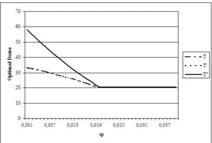
When the speed of de-sequestration is higher than the speed of sequestration, the optimal solution always consists in storing carbon in agricultural soils permanently, without any release (…gure 2). If the speed of de-sequestration was lower, it would be optimal to store carbon during a longer period of time and then release some carbon. For s = 0:02 and s0 _{= 0:01 for instance, carbon is stored in}

the soils during about 30 years, then release begins immediately and stops 12 years or so later. For s = 0:02 and 8s0 > s; the computation of the total value function shows that the optimal solution is the …rst corner solution (T = T0_{= T}00_{). Carbon is stored during about 20 years and never released.}

These results can be explained intuitively. If carbon release is a very slow process (slower than storage), de-sequestration induces an immediate bene…t as the cost associated to sequestration dis-appears, while the damage will appear only gradually. The parameter s0 acts as a discount rate concerning the damage. However, physical data of the sequestration process (s0 > s) rule out this kind of solution. Then, when de-sequestration is fast, it is never optimal to release carbon after having stored it. Optimal sequestration is permanent.

Figure 2: The optimal dates

With the assumption s = s0 _{= 1; in other terms when the dynamics of sequestation is ignored (case} studied by Feng et al. (2002)), the optimal sequestration is equivalent to half the physical potential sequestration (T = 50 years , A = 500 Mha). Whereas this optimal e¤ort corresponds to the …fth of the potential (T = 20 years , A = 200 Mha) for speeds of sequestration and de-sequestration close to the empirical French ones (s = 0:02 and s0 = 0:03): We see that the error made when not taking into account the dynamics of sequestration is very signi…cant, with an error coe¢ cient (1 +r_s) of 2:5 for our calibration.

Figures 3 and 4 show respectively the ‡ow of carbon emissions trapped and the additional carbon stock stored when we assume that these last values of s and s0_{are good proxis for the world conditions}

and for these two sequestration e¤orts (T = 50 and T = 20).

Figure 3: Flow of carbon trapped

Figure 4: Additional carbon stock sequestered

The additional carbon stock sequestered converges to a steady level of 7.5 GtC when we don’t take the dynamics of the physical process into consideration in the determination of the optimal policy (T = 50), while the optimal long term level is only 3 GtC (T = 20). The omission of the dynamic process leads to a very signi…cant over-sequestration.

5

Conclusion

This paper takes explicitely into account the temporality of sequestration. Its …rst contribution is technical. We solve an optimal control problem with two stages and a dissymmetric dynamic process. The second contribution is empirical. We show that the error made when sequestration is supposed immediate can be very signi…cant. We also exhibit numerically the optimal path of sequestation, which must be permanent if sequestration is faster than de-sequestration, for speci…c bene…t, damage and cost functions, and a calibration that mimics roughly the world conditions.

Interesting extensions would consist in considering factors that could make the optimal sequestation temporary, even in the case of a release faster than storage, like technical progress in abatement, or technical progress in usual practices and not in sequestering practices, that could increase the cost of sequestration.

6

References

Benaïm M. and M.W. Hirsch (1996), “Asymptotic pseudotrajectories and chain recurrent ‡ows with applications”, Journal of Dynamics and Di¤ erential Equations, 8, 141–176.

European Climate Change Programme (2003), Working Group on Sinks Related to Agricultural Soils - Final report.

Feng H, J. Zhao and C. Kling (2002), “The Time Path and Implementation of Carbon Sequestration”, American Journal of Agricultural Economics, 84, 134–149.

Hénin S.et M. Dupuit (1945), “Essai de bilan de la matière organique du sol”, Annales Agronomiques, n 15; 147–157.

INRA (2002), Increasing carbon stocks in French agricultural soils?, Report for the French Ministry for Ecology and Sustainable Development, October.

IPCC (2000), Land use, Land-use change and forestry (LULUCF), Cambridge University Press, U.K. Lal R., J.M. Kimble, R.F. Follet and C.V. Cole (1998), The potential of US cropland to sequester carbon and mitigate the greenhouse e¤ ect. Ann Arbor Press, Chelsea, MI.

Saglam H.C. (2002), “Optimal pattern of technology adoption under embodiement with a …nite plan-ning horizon: A multi-stage optimal control approach”, IRES, Université Catholique de Louvain. Smith P., J.U. Smith and D.S. Powlson (1996), Soil Organic Matter Network: 1996 Model and Ex-perimental Metadata. GCTE Report 7, GCTE Focus 3, Wallingford, Oxon.

Tomiyama K. (1985), “Two-Stage Optimal Control Problems and Optimality Conditions”, Journal of Economic Dynamics and Control, 9, 317–337.

Tomiyama K. and R. Rossana (1989), “Two-Stage Optimal Control Problems with an Explicit Switch Point Dependence: Optimality Criteria and an Example of Delivery Lags and Investment”, Journal of Economic Dynamics and Control, 13, 319–337.

A

The two-stage optimal control problem with an integral equation

of motion

The optimal control problem we study here has two distinctive features: (i) the accumulation of the state variable is dissymmetric and we must determine the switching point between the two stages of accumulation and desaccumulation; (ii) the motion of the state variable depends on the integral of a function of the past values of the control. The question is to check how to de…ne properly the Hamiltonian function corresponding to this problem, and how to write the …rst order necessary conditions and the matching conditions. We use a method close to the one developped in Saglam (2002) for a technology adoption problem.

A.1 Problem before T0

max V = Z T0 0 F (C(t); K(t); t)dt + V₊(K(T0); T0) _ K(t) = f (C(t); K(t); t) + Z t 0 g (C(z); t; z)dz; 0 t < T0 K(0) = K0 given, K(T0) free,

where K is the vector of state variables, C the vector of control variables, and T0 _{the switching time.}

Notice that this switching time appears explicitly in the equation of motion of the state variable. The Lagrangian of this problem is

= V + Z T0 0 (t) f (C(t); K(t); t) + Z t 0 g (C(z); t; z)dz K(t) dt;_

or, after changing the order of integration in the second term of the integral and integrating by parts the third one:

= Z T0 0 F (C(t); K(t); t)dt + Z T0 0 (t)f (C(t); K(t); t)dt + Z T0 0 Z T0 t (z)g (C(t); z; t)dz ! dt (T0)K(T0) (0)K(0) + Z T0 0 _ (t)K(t)dt +V₊(K(T0); T0):

Let the Hamiltonian be de…ned by

H (C(t); K(t); t; T0) = F (C(t); K(t); t) + (t)f (C(t); K(t); t) +

Z T0

t

Then we can write

= Z T0

0 H + _ (t)K(t) dt

(T0)K(T0) (0)K(0) + V₊(K(T0); T0):

Let (C (t); K (t)) be an optimal path 8t 2 [0; T0[ and T0 _{2 [0; 1[ : We perturb the C (t) path} by an arbitrary C(t); it generates, through the equation of motion, a perturbation of the K (t) path and of the optimal switching time T0 : C(t) = C (t) + " C(t); K(T0) = K(T0 ) + " K(T0), T0 = T0 + " T0 (Saglam (2002)). We then have @ @" = H jT0 + _ (T 0_)K(T0_{) T}0₊ Z T0 0 @H @C(t) C(t) + @H @K(t) K(t) + @H @T0 T0 dt + Z T0 0 _ (t) K(t)dt (T0) K(T0) _ (T0)K(T0) T0 + @V+ @K(T0₎ K(T 0_{) +}@V+ @T0 T 0 = _{H jT}0+ Z T0 0 @H @T0 dt + @V₊ @T0 ! T0+ Z T0 0 @H @C(t) C(t)dt + Z T0 0 @H @K(t) + _ (t) K(t)dt + @V₊ @K(T0₎ (T 0_{) K(T}0_):

Each component of this derivative must be equal to zero. This allows us to write the usual …rst order necessary conditions and the matching conditions:

…rst order necessary conditions:

@H @C(t) = 0 @H @K(t) + _ (t) = 0 matching conditions: H jT0 + Z T0 0 @H @T0 dt + @V₊ @T0 = 0 @V₊ @K(T0₎ (T 0_{) = 0:}

A.2 Problem after T0

max V+ = Z ₁ T0 F+(C(t); K(t); t)dt _ K(t) = f+(C(t); K(t); t; T0) + Z t T0 g+(C(z); t; z; T0)dz; T0 t K(T0) given.

Lagrangian of this problem: + = V++ Z ₁ T0 + (t) f+(C(t); K(t); t; T0) + Z t T0 g+(C(z); t; z; T0)dz K(t) dt_ = V++ Z ₁ T0 + (t)f+(C(t); K(t); t; T0)dt + Z ₁ T0 Z ₁ t +(z)g+(C(t); z; t; T0)dz dt lim t!1 +(t)K(t) +(T 0_)K(T0_{) +} Z ₁ T0 __+(t)K(t)dt: De…nition of the Hamiltonian:

H+(C(t); K(t); t; T0) = F+(C(t); K(t); t) + +(t)f+(C(t); K(t); t; T0) +

Z ₁

t

+(z)g+(C(t); z; t; T0)dz:

First order necessary conditions:

@H+

@C(t) = 0

@H+

@K(t)+ _+(t) = 0: We can write the objective as

+= Z ₁ T0 H+ + _+(t)K(t) dt lim t!1 +(t)K(t) +(T 0_)K(T0_{) :} Besides, we have dV₊ dT0 = @V₊ @K(T0₎ @K(T0₎ @T0 + @V₊ @T0; with dV₊ dT0 = d ₊ dT0 = _{H+ T0} _₊(T0)K (T0) + Z ₁ T0 @H+ @T0 dt + +(T0) @K(T0) @T0 + _+(T0)K (T0): So we can write @V₊ @K(T0₎ = +(T 0₎ @V₊ @T0 = H+ T0 + Z ₁ T0 @H+ @T0 dt:

Finally, the matching conditions can be written as follows:

(T0) = ₊(T0) H jT0+ Z T0 0 @H @T0 dt = H+ T0 Z ₁ T0 @H+ @T0 dt: Transversality condition: lim t!1 +(t)K(t) = 0:

A.3 Application

The previous results are applied to our problem, with the following de…nition of the variables and functions: C(t) = E(t) a(t) ! ; K(t) = S(t) A(t) ! ; F (C(t); K(t); t) = e rt(B(E(t)) D(S(t)) C(A(t))) f1 (C(t); K(t); t) = S(t) + E(t) f2 (C(t); K(t); t) = a(t) g1 (C(z); t; z) = ecsa(z)e s(t z) g2 (C(z); t; z) = 0 F+(C(t); K(t); t) = F (C(t); K(t); t) f1+(C(t); K(t); t; T0) = S(t) + E(t) ecs Z T0 0 a(z)e s(t z)dz f2+(C(t); K(t); t; T0) = b(t) g1+(C(z); t; z; T0) = ecb(z) se s(t (z))+ s0(1 e s(z (z)))e s 0_{(t z)} g2+(C(z); t; z; T0) = 0:

B

Analytical solution for the speci…c functional forms when

s

s

B.1 Interior solution

We …rst show that there is no interior solution for s0 s: Equations (61) and (62) imply

a(T00 _T0₎ r + a r2 1 e r(T00 _T0₎ = ec s0 (r + )(r + s0₎ 1 r(s0 _s) s0_{(r + s)}e s(2T00 _{T T}0₎ ec s0 (r + )(r + s0₎ 1 r(s0 s) s0_{(r + s)}e s(T0 _{T )} ecs r(s0 _s) (r + )(r + 2s)(r + s)(r + s0₎e s(T0 _{T )} 1 e (r+2s)(T00 T0) ;

which can be written, with X = T00 _T0 _{0; F (X) = 1 e} rX _{rX and G(X) = 1 e} 2sX

s r+2s 1 e (r+2s)X _; a r2F (X) = ec r(s0 _s) (r + )(r + s)(r + s0₎e s(T0 _{T )} G(X):

The LHS of this equality has the same sign as F (X); and the sign of the RHS depends on the sign of s0 s and G(X):

We show easily that F (X) 0 and G(X) _{0 8X} 0 : F (0) = 0 and F0(X) = r(e rX 1) < 0 8X > 0; G(0) = 0 and G0(X) = se 2sX(2 e rX_{) > 0 8X} 0:

When s0 > s; the only solution is then X = 0 i.e. T00 = T0. For s0 = s the equality reduces to F (X) = 0; and the only solution is again T00_{= T}0_.

For s0 s and T00 = T0; equations (61) and (62) become identical. The optimal dates T and T0 are then solution of the system composed of this last equation and (60):

8 < : aT r = (r+ )(r+s)ec s 1 e (r+s)(T0 _{T )} aT r = ec s 0 (r+ )(r+s0₎ 1 r(s0 s) s0_(r+s)e s(T 0 _{T )} :

The elimination of aT_r between these two equations yields r(s0 s)

r + s0 1 e

s(T0 _{T )}

= se (r+s)(T0 T );

which is impossible for T0 _{2 [T; 1[ since the LHS is positive and the RHS strictly negative.}

B.2 Corner solutions

We now examine the corner solutions.

There can …rst exist a corner solution before T0_{: Then, equations (61) and (62) are valid and imply}

as before T00 = T0; i.e. no de-sequestration. The date T at which sequestration stops can take two values: T0 or B_a:

If T = T0; (61) and (62) become identical and allow us to obtain ~

T2 = ec sr

a(r + )(r + s):

We obtain the same value ~T2 for a corner solution both before and after T0 (T = T0 = T00).

This solution is valid as long as ~T2< B_a, i.e. as long as _{(r+ )(r+s)}ec sr < B.

If T = B_a; we have e sT0 = e sBa (r + )(r + s)(r + s 0₎ ec s0_{r(s s}0₎ s0(r + s) r(s s0₎ ;

which requires B < _{(r+ )(r+s}ec s0r ₀₎. The solutions T = B_a and T = ~T2 can coexist for _{(r+ )(r+s)}ec sr < B < ec s0_r

(r+ )(r+s0). The corner solution before T0 (T = B

a) and T00 = T0 gives the same result.

There can also exist a corner solution after T0_{, T}00

1 = T2+ T0; but in this case we cannot obtain