Development of a variational flux inversion system (INVICAT v1.0) using the TOMCAT chemical transport model

HAL Id: hal-02954387

https://hal.archives-ouvertes.fr/hal-02954387

Submitted on 8 Oct 2020

HAL is a multi-disciplinary open access

archive for the deposit and dissemination of

sci-entific research documents, whether they are

pub-lished or not. The documents may come from

teaching and research institutions in France or

abroad, or from public or private research centers.

L’archive ouverte pluridisciplinaire HAL, est

destinée au dépôt et à la diffusion de documents

scientifiques de niveau recherche, publiés ou non,

émanant des établissements d’enseignement et de

recherche français ou étrangers, des laboratoires

publics ou privés.

(INVICAT v1.0) using the TOMCAT chemical transport

model

C. Wilson, M. Chipperfield, M. Gloor, F. Chevallier

To cite this version:

C. Wilson, M. Chipperfield, M. Gloor, F. Chevallier. Development of a variational flux inversion system

(INVICAT v1.0) using the TOMCAT chemical transport model. Geoscientific Model Development,

European Geosciences Union, 2014, 7 (5), pp.2485-2500. �10.5194/GMD-7-2485-2014�. �hal-02954387�

www.geosci-model-dev.net/7/2485/2014/ doi:10.5194/gmd-7-2485-2014

© Author(s) 2014. CC Attribution 3.0 License.

Development of a variational flux inversion system (INVICAT v1.0)

using the TOMCAT chemical transport model

C. Wilson1,2, M. P. Chipperfield2, M. Gloor1, and F. Chevallier3

1_{School of Geography, University of Leeds, Leeds, UK}

2_{School of Earth and Environment, University of Leeds, Leeds, UK}

3_{Laboratoire des Sciences du Climat et l’Environnement, CEA-CNRS-UVSQ, UMR8212, IPSL, Gif-sur-Yvette, France}

Correspondence to: C. Wilson (c.wilson@leeds.ac.uk) and M. P. Chipperfield (martyn@env.leeds.ac.uk)

Received: 27 September 2013 – Published in Geosci. Model Dev. Discuss.: 23 December 2013 Revised: 8 September 2014 – Accepted: 18 September 2014 – Published: 24 October 2014

Abstract. We present a new variational inverse transport model, named INVICAT (v1.0), which is based on the global chemical transport model TOMCAT, and a new correspond-ing adjoint transport model, ATOMCAT. The adjoint model is constructed through manually derived discrete adjoint algorithms, and includes subroutines governing advection, convection and boundary layer mixing, all of which are linear in the TOMCAT model. We present extensive testing of the adjoint and inverse models, and also thoroughly assess the accuracy of the TOMCAT forward model’s representation of atmospheric transport through comparison with observa-tions of the atmospheric trace gas SF6. The forward model

is shown to perform well in comparison with these obser-vations, capturing the latitudinal gradient and seasonal cycle of SF6 to within acceptable tolerances. The adjoint model

is shown, through numerical identity tests and novel trans-port reciprocity tests, to be extremely accurate in compari-son with the forward model, with no error shown at the level of accuracy possible with our machines. The potential for the variational system as a tool for inverse modelling is in-vestigated through an idealised test using simulated obser-vations, and the system demonstrates an ability to retrieve known fluxes from a perturbed state accurately. Using basic off-line chemistry schemes, the inverse model is ready and available to perform inversions of trace gases with relatively simple chemical interactions, including CH4, CO2and CO.

1 Introduction

Chemical transport models (CTMs) are powerful tools with which we can describe transport and chemical processes in the Earth’s atmosphere. CTMs provide global, three-dimensional (3-D) concentration fields of atmospheric trace gases and, through modification of model parameters and boundary conditions, they allow us to investigate the sensi-tivity of the state of the atmosphere to both anthropogenic and natural variations of these conditions. In order to accu-rately model the chemical composition of the atmosphere, it is important that a model’s input parameters, such as chem-ical reaction rates, meteorologchem-ical conditions and the mag-nitude and location of emissions of atmospheric species, are realistic. However, uncertainties still surround the spa-tial and temporal variation of the surface flux of some trace gases including, for example, carbon dioxide (CO2), methane

(CH4) and carbon monoxide (CO) (e.g. Gurney et al., 2002;

Frankenberg et al., 2008; Le Quéré et al., 2009; Kopacz et al., 2010). As well as enhancing the performance of atmospheric models, improving our estimates of the surface fluxes of at-mospheric species helps to broaden our knowledge of the processes through which trace gases are emitted, and there-fore improve our understanding of the interactions between anthropogenic activity, the biosphere, atmospheric composi-tion and climate.

There are a number of methods available for estimating the surface flux of atmospheric species. These can broadly be divided into two method types: bottom-up and top-down. Bottom-up methods are those that attempt to estimate fluxes either through direct measurements or by modelling the

processes which lead to flux of the species into the atmo-sphere. However, direct measurements of emission rates over relatively small regions are difficult to make and are subject to significant errors when extrapolated to global scales (Jung et al., 2011). Process modelling, meanwhile, requires con-siderable understanding of the complex procedures which lead to the emissions, and may also be subject to extrap-olation errors similar to those which affect the direct flux measurements. Top-down methods, in contrast, attempt to estimate emissions using information about the atmospheric distributions of the species and knowledge of atmospheric transport. This method has the benefit that the assimilation of observational data provides a constraint on the surface flux, assuming that the representation of atmospheric trans-port and chemistry is accurate. However, limitations of the top-down approach include insufficient global observational coverage and modelling inaccuracies (Dentener et al., 2003; Mikaloff Fletcher et al., 2004; Chen and Prinn, 2005). If mea-surements of the isotopic composition of a species are in-cluded in a top-down emission estimate, it may be possible to partition the distinct emission processes of the species. How-ever, since we currently have relatively poor global coverage of these isotopic observations (Dlugokencky et al., 2011), it is necessary that bottom-up and top-down processes must be used in tandem in order to gain full understanding of trace gas emission budgets. Since an atmospheric model, such as a CTM, is generally used to characterise the atmospheric transport and chemistry in order to relate the concentration fields to the surface flux, top-down techniques are usually referred to as “inverse modelling”. This is in contrast to for-ward modelling, which relates surface flux estimates to at-mospheric concentration fields. The increasing availability of satellite measurements of atmospheric constituents provides a powerful data set for use in data assimilation techniques such as inverse modelling. This, together with ongoing de-velopments of available computational power, means that in-verse techniques are increasingly achievable.

There exist a number of inverse modelling techniques available for constraining surface emissions of atmospheric species based on observations of atmospheric concentrations, many of which are detailed in Sandu and Chai (2011). The variational method used in this work is similar to the four-dimensional variational (4D-Var) method which has previ-ously been used in numerical weather prediction (NWP) (e.g. Le Dimet and Talagrand, 1986; Fisher and Courtier, 1995) in order to optimise model variables under the strong con-straint that the other sequences of the model state are ob-tained by prognostic equations. The variational inverse mod-elling method used in this study is not strictly identical to that of NWP 4D-Var data assimilation, since the inverse method optimises surface fluxes that are not updated as part of the prognostic equations of the forward model. It is true that the inverse method often includes the initial 3-D concentra-tion field of a species within the state vector, but this is usu-ally included as a side product of the inversion that ensures

consistency, and is not used after it has been computed. The term “4D-Var” has been used extensively in previous stud-ies to describe inverse schemes similar to that presented here (e.g. Meirink et al., 2008a, b; Bergamaschi et al., 2010). However, in order to avoid confusion with the NWP com-munity, the term “variational”, rather than “4D-Var”, will be used throughout this work. It should also be noted that we do not currently make use of the incremental variational method described by Courtier et al. (1994).

Variational techniques require the development of the ad-joint version of a CTM, which evaluates the sensitivity of a scalar metric of atmospheric concentration fields to input parameters such as surface fluxes. Through data assimila-tion, the inverse variational technique minimises, in a least-squares sense, a cost function which measures the difference between model predictions and observations, whilst also lim-iting changes made to existing knowledge of the surface fluxes as much as is reasonable.

This variational technique, and the related adjoint tech-nique, have both previously been applied in a number of studies relating to atmospheric science. Previous applica-tions have included Lagrangian transport models (e.g. Elbern et al., 1997), air quality data assimilation (e.g. Elbern and Schmidt, 2001; Carmichael et al., 2008) and Eulerian CTMs with full atmospheric chemistry schemes (e.g. Henze et al., 2007). Since the turn of the century, the combination of in-creased computational ability supplemented by large, high-resolution observational data sets provided by remote sens-ing has allowed atmospheric modellers to significantly ex-pand the potential of the inverse variational method. Pre-vious studies to have used this method in order to quan-tify surface fluxes of atmospheric species include Chevallier et al. (2005), Pan et al. (2007), Meirink et al. (2008b), Bergamaschi et al. (2010) and Bousquet et al. (2011).

This paper details the development and testing of a new variational inversion model which uses the TOMCAT CTM (Chipperfield, 2006) as its basis. TOMCAT has been ex-tensively used in the past for investigations into chemistry and tracer transport in the troposphere and stratosphere (e.g. Arnold et al., 2005; Monge-Sanz et al., 2007; Breider et al., 2010; Hossaini et al., 2010; Feng et al., 2011; Monks et al., 2012). The variational inverse modelling process initially re-quired the development of adjoint versions of the transport routines in TOMCAT, and the development of this adjoint model is also documented here. We also evaluate TOMCAT’s representation of atmospheric transport, since accuracy in this respect is crucial for the formulation of accurate sur-face flux estimates. One purpose of this work, therefore, is to quantify how well the new TOMCAT variational system performs as a tool to estimate surface fluxes in future appli-cations. The paper also includes a novel reciprocity test for the adjoint model, which is based upon the work of Hourdin and Talagrand (2006).

In Sect. 2 we describe the TOMCAT model, while in Sect. 3 we describe the variational inversion process. In

Sect. 4, we evaluate the representation of atmospheric trans-port in the TOMCAT model through comparisons with ob-servations of the trace gas sulfur hexafluoride (SF6), and we

describe the development and testing of a new adjoint model in Sect. 5. Finally, in Sect. 6, we report the construction and testing of the new variational inverse model.

2 The TOMCAT CTM

The TOMCAT model is an Eulerian, grid point, off-line three-dimensional (3-D) CTM, described in Chipperfield et al. (1993), Stockwell and Chipperfield (1999) and Chipperfield (2006). The standard horizontal model grid in the TOMCAT model is made up of regular longitudes and ir-regular Gaussian latitudes, whilst the vertical grid uses com-bined σ –p coordinates. Whilst the model typically has a hor-izontal resolution of 2.8◦_×2.8◦_{, with 60 vertical levels up} to 0.1 hPa, the high computational burden of the variational framework requires that a coarser resolution of 5.6◦×5.6◦, with 31 vertical levels up to 10 hPa is used whilst testing the inverse model. Previous studies have attempted to alle-viate the computational burden of the data assimilation or in-version process using reduced in-versions of non-linear models (Amsallem et al., 2013; Stefanescu et al., 2014), or with in-cremental optimisation using low-resolution linearised mod-els (Courtier et al., 1994). Further study is necessary to ex-plore the potential for these methods with the TOMCAT model. The model meteorology, including winds, tempera-ture and pressure data, is read in from ERA-Interim anal-yses provided by the European Centre for Medium-Range Weather Forecasts (ECMWF, http://www.ecmwf.int) (Dee et al., 2011) and transformed onto the TOMCAT model grid. The model uses a process split method, in which separate routines representing the different transport processes are carried out in sequence. In the standard model set-up used in this study, the atmospheric transport consists of routines based upon the Eulerian conservation of second-order mo-ments advection scheme developed by Prather (1986), a con-vection scheme based on that of Tiedtke (1989), and a bound-ary layer mixing scheme derived from that of Holtslag and Boville (1993). The advection routine is further split into three subroutines that each carry out tracer transport along one axis only (zonal, meridional or vertical). The model also contains the option of a full tropospheric chemistry scheme as detailed in Arnold et al. (2005), which may be replaced by a simpler “offline” scheme at the user’s discretion. The full chemistry scheme is not included in this work, however. A key characteristic of TOMCAT’s transport scheme is that it is linear in nature. This is beneficial, since non-linearities would complicate the development of the adjoint model.

3 Variational inverse modelling

The theory of the variational inversion technique with regards to estimating surface flux of atmospheric species has been well documented in studies such as Chevallier et al. (2005), Henze et al. (2007) and Meirink et al. (2008a). We summarise it here, as a full understanding of the theory is important to the analysis of the inverse model results. All notation follows that of Ide et al. (1997). The objective of variational inverse modelling is to optimise the value of a state vector, x, with n elements, in order to improve the prediction of the model in comparison with a set of m observations, y. The state vector in this case is a vector including the set of surface fluxes of atmospheric species, together with the initial 3-D atmospheric distribution of the species on the model grid resolution. Currently in TOMCAT, the surface flux has a monthly temporal resolution and spa-tial resolution dependent on the model grid. It is important to include the initial 3-D field within the state vector for long-lived species such as CH4 and CO2. The optimisation

is defined via a cost function, J (x), which accounts both for the accuracy of the model prediction compared with the observations and for departures from an a priori estimate of the state vector, xb. J (x) is defined as follows:

J (x) =1 2(x − x b₎T_B−1_{(x − x}b₎ +1 2(y − Hx) T_R−1_{(y − Hx), (1)}

where the superscriptTdenotes the transpose of a matrix and −1_{denotes its inverse. The matrix H represents the forward}

model simulation that maps from the state vector x onto the location and time of the observations in y. The n×n matrix B is the error covariance matrix for the a priori state vector, xb, while R is the error covariance matrix for the observations and has size m × m. R includes instrument error, representa-tion error and model error. For Bayesian theory to hold with Eq. (1), all errors must be assumed to be Gaussian and unbi-ased. The a priori state vector, xb, is in this case our current “best estimate” of the state vector, while the error covari-ance matrix B represents the uncertainty of this estimate. The cost function may be described in terms of the “background term” and the “observation term”, which refer to the contri-bution made by the departures made to the state vector and the model–observation differences, respectively. Finding the minimum value of the cost function is equivalent to finding the optimum value of x. There are different methods avail-able for solving this problem, and variational schemes use iterative methods in order to find the point at which the gra-dient of the cost function with respect to the state vector, no-tated ∇xJ (x), is zero. This can only occur at a stationary point (minimum or maximum) of J . That is, when

Numerically, difficulties arise in the calculation of HT, which is the transpose of the matrix H, since it is imprac-tical to find either of these matrices explicitly on the model grid resolution. Instead we use a forward model, M – in our case TOMCAT – together with a linear interpolation from the model grid onto the observation space in place of the matrix H in Eq. (1). Through linear interpolation from the model grid onto the latitude, longitude and altitude of each obser-vation in y at the time that the obserobser-vation was made, we thus obtain a mapping from the state vector onto the obser-vation space. Since the transport in TOMCAT is linear, the use of this model together with the linear interpolation onto y is exactly equivalent to the matrix H.

The forward model is, in reality, a set of discrete math-ematical operations and conditional statements, rather than a matrix operator, and we can therefore not explicitly find HTusing the forward model only. Instead, we use an adjoint model, M∗_{, as shown by Talagrand and Courtier (1987).} To-gether with an adjoint linear interpolation from the obser-vation space onto the model grid, the adjoint model is used instead of explicitly finding HT. The theory of adjoint mod-elling is expanded upon in the next section. Again, due to the linearity of TOMCAT transport, this adjoint mapping from the observations onto the state vector is equivalent to HT. The adjoint version of the TOMCAT model was written for use with the new inverse model. ∇xJ (x) can therefore be found as in Eq. (2) using the forward and adjoint models in place of H and HT. Once ∇xJ (x) has been found, it can be used in or-der to choose an appropriate descent direction along which to minimise J (x). This process of finding the Jacobian of J (x) and using it to minimise the cost function is repeated itera-tively until some convergence criterion is met. The iterative process of minimisation will be discussed further in Sect. 6. 3.1 Adjoint modelling

The forward model M can be defined such that, for a concen-tration field c at time ti,

c(ti+1) = M[c(ti)], (3)

where time ti+1 denotes one model time step after time ti. In practice, the model consists of parameterisations of vari-ous transport and chemical processes, and each of these pro-cesses is made up of a finite number of mathematical opera-tions, Mj:

M[c(ti)] = Y

j

Mj[c(ti)]. (4)

In our case, each operation Mjis linear and differentiable. However, this is not true for all models, many of which con-tain non-linear operators. Assuming however that each model operator M is differentiable, a first-order approximation of its first derivative, or Jacobian, can be represented by a tangent linear model (TLM), M0. The TLM simulates the propaga-tion of perturbapropaga-tions forward in time and is dependent upon

the model state at which the linearisation takes place. The TLM is therefore defined such that

δc(ti+1) = M0[c(ti)]δc(ti) =

∂M[c(ti)]

∂c δc(ti). (5)

Note that the model operator is differentiated with respect to the concentration field c, and not the perturbation δc. In practice, this means that elements of the forward model state must be made available in order to run the TLM. This pro-cess is known a “checkpointing”. Each mathematical opera-tion Mj must be individually differentiated to create Mj0:

δc(ti+1) = Y j M_j0[c(ti)]δc(ti) = Y j ∂Mj[c(ti)] ∂c δc(ti). (6)

As mentioned, if the model M is already linear, as with TOMCAT, then the TLM is identical to the forward model. TLM development and checkpointing are then unnecessary. From the TLM, the adjoint model (ADM), M∗, can be de-veloped. The adjoint model propagates variables backwards through time in order to give the sensitivity of a scalar metric of c (such as J ) to the model input parameters. M∗is defined such that, for an inner product h , i and for vectors u and v, it holds that

∀u, ∀v hM0u, vi = hu, M∗vi. (7)

When creating the adjoint model, it is necessary to choose whether to use the adjoint of the transport equations on which the forward model is based, known as a continuous adjoint, or to find the adjoint from the forward model code directly, known as a discrete adjoint. Sirkes and Tziperman (1997) showed that, when using a “leap-frog” advection scheme, their continuous adjoint differed from the actual numeri-cal gradient of J (x), which slowed down the minimisation, but that it did not introduce non-physical behaviour, such as a two-timestep leapfrog computational mode. Gou and Sandu (2011) carried out a comparison between the continu-ous and discrete adjoints for a piece-wise parabolic advection scheme. They found that the discrete adjoint in this case led to worse performance than the continuous adjoint for vari-ational applications in experimental settings, but that there was little difference in the performance of the two schemes in an inversion using real observational data. Recently, Haines et al. (2014) used an Eulerian backtracking method in order to combine the advantages of both the discrete and contin-uous adjoint formulations into a single adjoint model. We decided that we would use the discrete adjoint of TOMCAT for this work, in order to make it consistent with the forward model. However, further tests in the future should be carried out in order to examine the performance of the continuous and discrete adjoints of the TOMCAT advection scheme.

In practice, the forward model consists of several thousand lines of computer code, each carrying out a mathematical operation or creating a conditional statement or loop. TLM

and ADM codes can therefore be created from the forward code by hand or through the use of automatic code genera-tors. A variety of these are available, such as TAMC (http:// www.autodiff.com/tamc) and TAPENADE (www-sop.inria. fr/tropics/tapenade.html), which create a TLM or ADM from a supplied forward model without the need for the time-consuming hand-coding process. Whether coded by hand or automatically, the creation process may produce errors or inconsistencies in the adjoint code, due to human error or through bugs introduced in the automatic coding process (Nehrkorn et al., 2006), and it can often be more efficient to code by hand in the first place. A major problem with au-tomatic procedures is that they may also reduce the poten-tial for optimisation of the adjoint code, such as parallelisa-tion. Since the variational approach described here relies on a number of iterations of forward and adjoint model simu-lations being carried out, parallelisation of the model code may be necessary in order to carry out inversions with long inversion time-periods. It was therefore decided to develop the adjoint version of the TOMCAT model by hand, rather than through the use of an online tool, as this would allow a greater level of control over the format of the code, and a better understanding of the details of the development pro-cess. Other groups have previously detailed the development of adjoint versions of atmospheric models using continuous adjoints and automatic code generators (e.g. Meirink et al., 2006; Hakami et al., 2007; Henze et al., 2007; Huang et al., 2009).

For this work it was decided that only the TOMCAT rou-tines concerning atmospheric transport would be included within the inversion. The model’s full chemistry scheme was not included as this would significantly increase the run-ning time of the inverse program, which we initially intend to apply to species such as CO2, which is treated as a

pas-sive tracer, and CH4, which can be simulated using

speci-fied chemical destruction fields, and so do not require the full model chemistry scheme. It is currently intended that the full chemical adjoint scheme will be included at a later date. It was therefore necessary to produce adjoint versions of the TOMCAT model’s advection, convection and plane-tary boundary layer transport schemes, along with other sub-routines concerning the model’s calendar and initialisation.

Since each operation within every section of the model’s transport scheme was already linear, there was no need to produce a TLM. This meant that we could proceed directly to the production of the model’s adjoint. With the adjoint model completed, it was important to thoroughly validate each sub-routine against its equivalent in the forward model in order to ensure its accuracy. The details of this testing will be dis-cussed in Sect. 5.

4 Assessment of tropospheric transport in TOMCAT In order that the TOMCAT model may be used as an inverse modelling tool, it is important to assess the accuracy of the model’s representation of atmospheric transport. The varia-tional inversion process assumes that all model errors are Gaussian and unbiased, and therefore significant model bi-ases would propagate through the model and violate these basic assumptions.

Whilst the observation error covariance matrix R should theoretically take account of model transport error, in a vari-ational inverse simulation, in practice this is difficult to quan-tify and so it is usually assumed that model transport is ac-curate and unbiased when performing an inversion. Here we use observations of the atmospheric trace gas sulfur hexaflu-oride (SF6), together with output from multiple model

simu-lations at different grid resolutions in order to ascertain that the accuracy of the forward model transport is good enough to be used for inverse modelling. SF6 is useful for

investi-gating aspects of atmospheric transport, and has been used previously in a number of such studies (e.g. Gloor et al., 2007; Patra et al., 2009). It is especially suited to examin-ing interhemispheric transport, since its sources are almost exclusively located in the Northern Hemisphere (NH).

SF6, which is a potent greenhouse gas, is inert in the

tro-posphere and stratosphere, giving it an extremely long atmo-spheric lifetime which has been estimated to be between 800 and 3200 yr (Ravishankara et al., 1993; Morris et al., 1995). The only atmospheric sinks of SF6are a relatively slow

pho-tochemical destruction process and electron capture, both of which only occur in the atmosphere above 60 km, therefore having only a small impact on its atmospheric concentration (Reddmann et al., 2001). Hall and Waugh (1998) found that ignoring the effect of mesospheric destruction when simulat-ing SF6may lead to over-estimation of SF6concentration in

the high-latitude middle stratosphere (above 30 km), but only has a small effect elsewhere.

This property is one of many which make SF6 a good

tracer for testing the simulated long-term atmospheric trans-port in CTMs. The fact that SF6is inert in the troposphere

and stratosphere means that there is no need to include chem-ical processes in the model. Also, the release of SF6into the

atmosphere is almost entirely anthropogenic in nature. This means both that emissions are fairly constant in time (Levin et al., 2010), with a negligible seasonal cycle (Olivier and Berdowski, 2001), and that we can produce spatially accu-rate surface emission estimates by distributing sales num-bers within each nation according to electrical energy use (Olivier, 2002).

The TOMCAT model previously submitted the results of long-term SF6simulations to the TransCom CH4

intercom-parison project (Patra et al., 2011), where it captured the sea-sonal cycle of SF6 at three ground-based observation sites

to a high level of statistical significance, and reproduced the interhemispheric gradient of SF6 to within 0.05 parts per

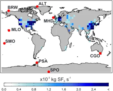
SPO PSA CGO SMO MLO MHD ALT BRW x10 kg SF s-3 -1 6

Fig. 1. Emissions ofSF6(×10−3kggridcell−1s−1) on the5.6◦×5.6◦TOMCAT grid for the year 2008.

Locations of NOAA surface stations used in this study are also shown.

35

Figure 1. Emissions of SF6 (×10−3kg grid cell−1s−1) on the

5.6◦×5.6◦TOMCAT grid for the year 2008. Locations of NOAA surface stations used in this study are also shown.

trillion (ppt). However, those simulations were carried out using the standard TOMCAT model grid resolution (2.8◦× 2.8◦with 60 vertical levels up to 0.1 hPa), whilst the varia-tional inverse model will initially be run using a coarser res-olution (5.6◦×5.6◦, 31 vertical levels up to 10 hPa) in or-der to reduce simulation times and memory requirements as much as possible. Therefore, new SF6simulations were

car-ried out with the TOMCAT model at this coarse resolution in order to assess the effect that reducing the model’s reso-lution has on its performance. For these simulations, the 3-D SF6 field was initialised on 1 January 1988, with initial

values provided by TransCom, and ran up until 31 Decem-ber 2010, with full 3-D output every 3.75 days. The model timestep was 60 min. We linearly interpolated the TransCom initial concentration field from a 2.8◦×2.8◦horizontal grid with 60 vertical levels to the coarser 5.6◦×5.6◦, 31 level TOMCAT grid. Due to the long spin-up time for this simu-lation, the initial field should not significantly influence the results in the more recent years. Emissions were also sup-plied by TransCom, and were originally taken from the Emis-sion Database for Global Atmospheric Research (EDGAR), Version 4.0 (Olivier and Berdowski, 2001), and scaled as in Reddmann et al. (2001). Figure 1 shows annual mean SF6

emissions for the year 2008 on the 5.6◦_×5.6◦ _TOMCAT model grid, showing that the majority of SF6emissions are

from NH industrialised countries. Model output was com-pared with flask measurements of surface SF6from remote

station sites in the National Oceanic and Atmospheric Ad-ministration (NOAA) network, who have taken weekly mea-surements of SF6 at a number of stations since 1995. The

locations of the stations used for comparison with the model are also shown in Fig. 1. Measurements have an accuracy of approximately 0.04 ppt.

Table 1. Pearson’s correlation value (r_5.6 and r_2.8) and

root-mean-square error (RMSE_5.6 and RMSE_2.8) for modelled and observed seasonal cycle of SF6at eight surface stations, shown in

Fig. 2, for two different model grid resolutions.

Station r_5.6 r_2.8 RMSE_5.6 (ppt) RMSE_2.8 (ppt) ALT 0.29 0.58 0.018 0.015 BRW 0.52 0.64 0.012 0.011 MHD 0.60 0.67 0.020 0.015 MLO 0.36 0.32 0.017 0.018 SMO 0.85 0.89 0.014 0.009 CGO 0.13 0.53 0.011 0.009 PSA 0.22 0.42 0.012 0.011 SPO 0.49 0.75 0.012 0.010

Figure 2 shows the modelled and observed mean de-trended seasonal anomalies of SF6at each station at both the

2.8◦×2.8◦and 5.6◦×5.6◦grid resolutions. Table 1 shows the Pearson’s correlation value (r) and the root-mean-square er-ror (RMSE) between observed and modelled SF6anomalies

at each station for both model resolutions. For both modelled and observed SF6, in order to display only the seasonal

cy-cle due to transport, the linear trend displayed by SF6at the

South Pole station (SPO), the site furthest from the source regions, was removed from all data. The modelled and ob-served SF6 was averaged over the years 2005 to 2010, and

the mean value at each station over this time period was sub-tracted. This figure shows that switching to the lower reso-lution does not have a significant impact upon the model’s representation of the seasonal cycle, especially in the SH. Prather (1986) showed that the advection scheme used in the model performs well at low resolutions and is relatively non-diffusive. In the NH, however, the proximity of the majority of SF6 emissions mean that the larger grid boxes produce

a diffusive effect as emissions are more rapidly mixed across grid boxes, which slightly alters the model concentrations. Differences between the two resolutions are never greater than 0.03 ppt, however. The greatest difference between the two resolutions is at the MHD station, due to the fact that this particular station, located on the west coast of Ireland, is sub-ject to numerical diffusion of high UK and Irish emissions through the model grid box to different extents depending on the grid box size. Due to the effect of these local emis-sions, MHD has the largest RMSE of any of the stations, but the correlation is relatively high (≥ 0.60), since the timing of the variations is captured well in the model. At the two Arctic stations, ALT and BRW, there appears to be a system-atic underestimation of the negative seasonal anomaly dur-ing September and October. This may indicate strong model transport into the Arctic during these months, or weak trans-port away from the region.

SH sites such as CGO, PSA and SPO have relatively weak seasonal cycles, and the model shows extremely lit-tle variation around the mean in the SH. Some SH seasonal

obs mod, 5.6o mod, 2.8o J F M A M J J A S O N D J F M A M J J A S O N D ALT BRW MHD MLO SMO CGO SPO PSA

SF

anomoly (ppt)

month

Fig. 2. Modelled and observed monthly meanSF6anomoly (ppt) averaged over the period 2005–2010.

The blue line represents modelledSF6 using the2.8◦× 2.8◦TOMCAT model grid, while the red line

shows results for the5.6◦_×5.6◦_{model grid. Black dots represent flask observations from NOAA surface}

station sites, and error bars show one standard deviation of the monthly mean of the observations over the six-year period.

36

Figure 2. Modelled and observed monthly mean SF6anomaly (ppt)

averaged over the period 2005–2010. The blue line represents mod-elled SF6using the 2.8◦×2.8◦TOMCAT model grid, while the

red line shows results for the 5.6◦×5.6◦ model grid. Black dots represent flask observations from NOAA surface station sites, and error bars show one standard deviation of the monthly mean of the observations over the 6-year period.

variation may be missing in the model, as the observations display larger anomalies than those produced by the simu-lation. This may indicate that there is too much homogene-ity in the modelled SH troposphere. The decrease in reso-lution produces very little impact on the modelled seasonal cycle at these stations. Due to the weak seasonal cycle, small model–observation correlations are not necessarily represen-tative of poor model performance, and the fact that the RMSE is less than 0.012 ppt at each of these stations indicates that the model is representing transport to the SH well. SMO dis-plays positive anomalies in December through to March and negative anomalies for the rest of the year due to its posi-tion relative to the Intertropical Convergence Zone (ITCZ), which is the meteorological (rather than the notional 0◦₎ boundary between the NH and SH. As the position of the ITCZ varies throughout the year due to the changing loca-tion of the sun’s zenith point, SMO alternates between sam-pling NH and SH air. This oscillation is reproduced in both of the model simulations, with correlations greater than 0.8 produced by each. MLO displays a biannual seasonal cycle, due to the increased influence of SH air at MLO during the NH summer and winter (Lintner et al., 2006), and the model

latitude

0

-30

-60

-90

30

60

90

S

[ppt]

F

6.0

5.5

5.0

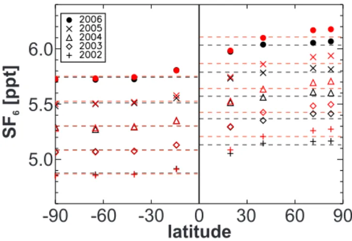
Fig. 3. Modelled and observed annual meanSF6concentrations (ppt) at different latitudes for the period

2002–2006. The black symbols represent observations at eight surface stations, while the red symbols show the equivalent modelled concentrations using the5.6◦_{× 5.6}◦_{model grid. Different years are}

rep-resented by different symbols, as shown in the legend. The dotted lines represent the observed (black) and modelled (red) NH and SH mean concentration for each year.

37

Figure 3. Modelled and observed annual mean SF6concentrations

(ppt) at different latitudes for the period 2002–2006. The black symbols represent observations at eight surface stations, while the red symbols show the equivalent modelled concentrations using the 5.6◦×5.6◦model grid. Different years are represented by different symbols, as shown in the legend. The dotted lines represent the ob-served (black) and modelled (red) NH and SH mean concentration for each year.

produces the same semi-annual variation, albeit with smaller negative SF6 anomalies during January and February. The

correlations here are relatively low (0.32–0.36) due to this fact.

Figure 3 shows the annual mean modelled and observed SF6at eight surface stations located at different latitudes for

the years 2002 to 2006. The modelled SF6is taken from the

simulation which used the 5.6◦_×5.6◦_{grid resolution, and in} order to remove any bias caused by the model initialisation, the mean model bias at SPO for January 2000 was removed uniformly from all modelled SF6concentrations at all times.

The model captures the annual increase of SF6at the surface

well, but the interhemispheric difference (IHD) is too large in the model compared with the observations. The mean ob-served IHD is approximately 0.28 ppt for this period, while the mean modelled IHD is 0.34 ppt, which is approximately 18 % too high. This shows that interhemispheric transport in TOMCAT is likely too slow.

Overall, the tracer transport in the TOMCAT model per-forms well in comparisons with observed SF6. Comparisons

with flask samples at station sites provide a validation of the large-scale transport in the model such as interhemispheric and zonal transport and representation of seasonal large-scale atmospheric variations such as the ITCZ. The simulations reproduce the phase and amplitude of the seasonal cycle at most stations. Some SH seasonal transport variations are not reproduced in the model, and model transport in the Arc-tic may not be strong enough during the NH autumn. How-ever, the timing and magnitude of the effect of the ITCZ is captured well. The observation accuracy of 0.04 ppt at these stations is close to the absolute seasonal variation in many

places, and the model is always within this level of accuracy. Work is always ongoing to improve the TOMCAT model’s representation of physical processes, and the adjoint model will be similarly maintained in the future.

5 Construction and validation of the adjoint model As discussed in Sect. 3, in order to use the TOMCAT model in a variational framework, it is first necessary to produce an adjoint version of the model. In order to reduce the run-ning time of the adjoint model, the forward TOMCAT model was altered so it saved any variables at each model timestep that are also needed by the adjoint model. This meant that these variables did not have to be recalculated for use in the adjoint model. Adjoint versions of the advection, convection and boundary layer transport schemes were produced, and each of the new forward and adjoint routines were coded by hand. Each subroutine was individually and thoroughly tested to confirm its accuracy in relation to the original for-ward version of the routine. They were then combined to pro-duce the full adjoint version of the TOMCAT model, known as ATOMCAT. The accuracy of the full adjoint model was then also tested.

5.1 Adjoint model tests

This section describes the tests which were used in order to assess the accuracy of ATOMCAT. If the transport in the ad-joint model is not exactly accurate, then at best, it will intro-duce errors into the a posteriori estimate of the state vector. In the worst case, the cost function may not converge at all. Three different tests were carried out, the first of which con-firmed that the adjoint identity equation, as defined in Eq. (7), held for ATOMCAT. This first test should in fact be suffi-cient to be assured of the accuracy of the adjoint model, but a second test was also performed which ensured that tracer transport in ATOMCAT is reciprocal to that of the TOM-CAT model, a property that should hold for adjoint models (Hourdin and Talagrand, 2006). This test is an extension of the adjoint identity test, and provides further validation of the adjoint transport over longer time periods. Finally, a test we refer to as the “alpha test”, described in Navon et al. (1992), was carried out. This tested the accuracy of the adjoint model using a Taylor expansion of the cost function. While none of these tests are exhaustive, in the sense that they cannot pos-sibly be carried out using all possible input values, they do provide a strong endorsement of the accuracy of the adjoint model.

For each individual subroutine, it was checked that the identity shown in Eq. (7) held. In practice, it was checked that the following identity held up to the level of accuracy possible due to the rounding error introduced on the machine used to perform the simulation, known as the machine ep-silon:

∀u, ∀v hM 0_{u, vi}

hu, M∗_vi=1. (8)

Equation (8) was tested for each of the three subroutines representing advection in each dimension, and also for the convection and boundary layer mixing schemes, as well as for the full ATOMCAT model. The input variable for the for-ward subroutine, u, was defined as a normally distributed random variable, and in the input variables for the adjoint subroutines were defined to be equal to the output from the corresponding forward subroutine, M0(u). The identity in Eq. (8) is then

||M0(u)||2

hu, M∗_(M0_(u))i=1. (9)

The ADM was tested based on Eq. (9) using 10 different random initialisations for 480 iterations (equal to 20 model days) of each subroutine. We found that for each subroutine and each initialisation, the identity given in Eq. (9) holds up to machine epsilon, strongly indicating that the adjoint model has been accurately coded from the forward model. The level of accuracy of the results of this test implies that the adjoint model is likely to be correct.

5.2 Reciprocity of atmospheric transport

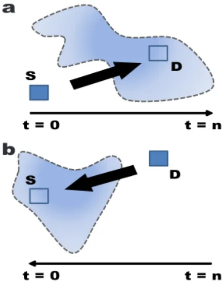
In order to further test the accuracy of the adjoint transport in ATOMCAT, the property of reciprocity of model trans-port was investigated. It has been previously discussed that for a linear model, transport in the adjoint model is recipro-cal to transport in the forward model (e.g. Hourdin and Tala-grand, 2006; Hourdin et al., 2006). This result is equivalent to Eq. (7) and implies that the accuracy of ATOMCAT may be tested by examining the reciprocity of its transport. The tests in this section are therefore extensions of those performed in Sect. 5.1, and examine the accuracy of the adjoint model over multiple model time steps. The reciprocity test posits that if the adjoint model is initialised with a mass, m, of tracer in any given model grid box, D, and integrated backwards through time from time tn to time t0, then the mass in any

other specified grid box S at t0is equal to that which is found

in D if the forward model is integrated from t0to tnafter be-ing initialised with mass m of tracer in grid box S. Figure 4 shows a schematic of this theory. Due to the high computa-tional burden of adjoint modelling and the increased simula-tion time required to carry out both forward and adjoint sim-ulations, the reciprocity of tracer transport in the ATOMCAT model was examined on two different timescales. The adjoint transport over 1 day was examined from every surface grid box, while longer simulations were carried out which inves-tigated adjoint transport from selected grid boxes only.

In order to test the short-term reciprocity of the ADM transport, separate forward simulations were carried out in

t = 0 t = n S D D

a

b

Fig. 4. Diagram showing the principle of reciprocity of atmospheric transport using an adjoint model. (a) shows the dispersion of a massm of tracer in the forward model, released from box “S” at time t = 0

aftern model timesteps. Concentration is indicated by colour intensity. (b) shows the equivalent adjoint

transport for a massm of tracer, released from grid box “D” at time n, integrated backwards to time 0.

The mass of tracer in box “D” in (a) at time n and in box “S” in (b) at time 0 is identical.

38

Figure 4. Diagram showing the principle of reciprocity of

atmo-spheric transport using an adjoint model: (a) shows the dispersion of a mass m of tracer in the forward model, released from box “S” at time t = 0 after n model time steps; concentration is indicated by colour intensity; (b) shows the equivalent adjoint transport for a mass m of tracer, released from grid box “D” at time n, integrated backwards to time 0. The mass of tracer in box “D” in (a) at time n and in box “S” in (b) at time 0 is identical.

which one surface grid box, S, was initialised with an (ar-bitrary) concentration of tracer mass of 100 kg, with zero mass elsewhere. One separate simulation was performed for each surface grid box. After the simulation period of 1 day (1 July 2008) was complete, the location D and value mD of the maximum tracer mass in each simulation was noted. Following this, separate adjoint simulations were carried out in which a pulse of 100 kg was placed into each box D and the ADM was integrated backwards over the same day. In an accurate adjoint model, the total mass, mS contained in grid box S at the end of the adjoint simulation should be equal to mD. All forward and adjoint simulations included all of the transport processes available in the model. This was repeated for every surface grid box, using the 5.6◦×5.6◦resolution (giving 64×32 = 2048 simulations). For each simulation, the values of mDand mSwere exactly equal at machine epsilon, indicating that the adjoint transport in ATOMCAT is correct over short timescales.

In order to test the reciprocity property of adjoint transport in the ATOMCAT model over a longer time period, simula-tions were carried out in which the reciprocity experiment described above was repeated over a time period of 1 month (July 2008), but for 10 surface grid boxes Sn, 1 ≤ n ≤ 10, only. This test was carried out only at certain locations due to the computational burden and time that a more large-scale test would necessitate. Again, at the end of the forward sim-ulation the grid box Dn with the largest mass of tracer mnD was found and chosen to be the initial grid box for an adjoint simulation over the same month. Figure 5 shows the results

of this experiment for one of the sites chosen for the emis-sion pulse’s starting point, with the location of the other sites marked in the uppermost panel. Figure 5b shows the tracer mass distribution at the seventh vertical model level from the surface on 31 July, 1 month after release from the grid box marked “S”, located at 84.4◦W, 30.5◦N. The grid box con-taining the maximum tracer mass at this time is marked “D”. Figure 5c meanwhile, displays the surface level distribution of tracer mass on 1 July, at the end of an adjoint simulation initialised on 31 July with a tracer mass of 100 kg released from grid box “D”. In this case, and in each of the other cases, the tracer masses mn_Sand mn_D are exactly equal at ma-chine epsilon. Again, this implies that the tracer transport in ATOMCAT is consistent with that of the forward model, and suggests that over a longer time period the adjoint model is representative of the forward model transport to a high level of accuracy.

Finally, we carried out the accuracy test described by Navon et al. (1992), in which the Taylor series of the cost function is evaluated. Taylor’s theorem states that

J (x + αδx) = J (x) + αδxT∇_xJ (x) + O(δx2), (10)

where α is a small scalar and δx is a vector of the size of x. Rewriting this equation, we have

φ (α) =J (x + αδx) − J (x)

αδxT_{∇xJ (x)} =1 + O(δx). (11)

Therefore, for values of α that are small, but not too close to the order of accuracy of the machine, φ(α) should be close to 1. We tested this identity by letting the state vector, x, be the emissions of SF6 on the TOMCAT model grid, shown

in Fig. 1. Note that, for this test, we did not include the ini-tial atmospheric concentrations in the state vector. We also discarded the background term of the cost function, as it would not affect the result, and generated a set of pseudo-observations, y, by running the forward model for 7 days from 1 July 2008 and multiplying the resultant 3-D field by a factor of 1.5. We defined δx to equal x/10, and let α vary between 1×10−14 and 1. Figure 6 shows the results of this test. It is clearly seen that for values of α between 1×10−11 and 1×10−2, a unit value of φ(α) is obtained. As previously explained, whilst these tests do not completely validate the accuracy of the adjoint model, the perfect level of accuracy attained very strongly suggests that the adjoint transport in ATOMCAT is correct.

6 The TOMCAT variational inverse model

Once ATOMCAT had been completed and fully tested, it could be included in the new variational inverse version of the TOMCAT model, named INVICAT. The variational scheme used was based upon the system developed by Chevallier et al. (2005), which makes use (non-exclusively)

b

c

x 10

a

Fig. 5. (a) Locations of grid-cells from which tracer is released for ten individual one-month transport

reciprocity tests described in Sect. 5. (b) Tracer mass (kg) at the 7th model level from the surface (approximately 2.6km) at the end of a 30 day forward simulation initialised with a mass of 100 kg at the

surface below the grid cell labelled “S” on 1 July 2008. The mass of tracer in the grid cell labelled “D”

is10.807×10−2_{kg. (c) Surface tracer mass (kg) at the end of a 30 day adjoint simulation initialised with}

a mass of 100kg above grid cell labelled “D” on 31 July 2008. The tracer mass in “S” at the surface is

also equal to10.807 × 10−2_kg.

39

Figure 5. (a) Locations of grid cells from which tracer is released

for 10 individual 1-month transport reciprocity tests described in Sect. 5. (b) Tracer mass (kg) at the seventh model level from the surface (approximately 2.6 km) at the end of a 30-day forward sim-ulation initialised with a mass of 100 kg at the surface below the grid cell labelled “S” on 1 July 2008. The mass of tracer in the grid cell labelled “D” is 10.807 × 10−2kg. (c) Surface tracer mass (kg) at the end of a 30-day adjoint simulation initialised with a mass of 100 kg above grid cell labelled “D” on 31 July 2008. The tracer mass in “S” at the surface is also equal to 10.807 × 10−2kg.

of the M1QN3 minimisation program, described by Gilbert and Lemarechal (1989), in order to minimise the cost func-tion J (x). This program uses the Limited-memory Broyden– Fletcher–Goldfarb–Shanno (L-BFGS) algorithm which re-duces the amount of computer memory necessary to find the optimal solution of a problem (Perry, 1977; Shanno, 1978; Nocedal, 1980).

The minimisation program is first called once the initial value and gradient of the cost function have been found. It is then repeated iteratively until the cost function or its gradient have met some pre-defined convergence criterion, when the program returns the a posteriori state vector. As in Chevallier et al. (2005), a preconditioning transformation is applied to the state vector in order to optimise the speed of the min-imisation. Instead of minimising x directly, the variable z is defined such that z = B−1/2(x −xb), and this variable is min-imised instead. This increases the efficiency of the minimisa-tion by reducing the ratio of its largest and smallest eigenval-ues (known as the condition number) of the Hessian of the cost function (∇2J (x)) (e.g. Andersson et al., 2000).

At each iteration k, k ≥ 1, the program determines an ap-propriate descent direction, dk, of J (x) at xk, where xk is

10−14 ₁₀−12 ₁₀−10 ₁₀−8 ₁₀−6 ₁₀−4 ₁₀−2 ₁₀0 α 0.8 0.9 1.0 1.1 Φ ( α ) −14 −12 −10 −8 −6 −4 −2 0 log10(α) −4 −3 −2 −1 0 log 10 ( Φ ( α )−1)

Fig. 6. Verification of the alpha test. (a) variation ofφ(α) with respect to α; (b) variation of log10(φ(α)−

1) with respect to log10(α).

40 (a)

(b)

Figure 6. Verification of the alpha test. (a) variation of φ (α) with

re-spect to α; (b) variation of log₁₀(φ (α)−1) with respect to log₁₀(α).

the updated state vector at iteration k. A quasi-Newtonian (QN) method is used in order to choose an appropriate de-scent direction. This has the advantage over other methods of not needing an exact line search in order to find the mini-mum along dk, although it requires a relatively large amount of computer memory when compared to conjugate gradient methods (Gilbert and Lemarechal, 1989). INVICAT’s min-imisation program chooses the descent direction with the value dk= −Wkgk, where Wkapproximates the inverse Hes-sian of J (xk), and gk is the gradient of the cost function at xk. Once this descent direction is chosen, the step size, αk, to be taken along this direction is determined by the line search procedure. At the next iteration the state vector therefore has the form xk+1=xk+αkdk.

Initially, αk is set to equal hg2J (xk,gkk)i, before iteratively being

quickly reduced to an appropriate length to find the mini-mum along dkby testing the Wolfe conditions, which are as follows:

J (xk+αkdk) ≤ J (xk) + ω1hgk,dki, (12)

hgk+1,dki ≥ω2hgk,dki, (13)

where it is necessary to have 0 < ω1<1₂ and ω1< ω2<1.

For this study, values of ω1=0.0001 and ω2=0.9 were

cho-sen. The line-search algorithm iteratively reduces the value of αk until Eqs. (12) and (13) both hold.

Figure 7 shows a flowchart representing the steps under-taken by INVICAT model in order to find the a posteriori flux estimate. As mentioned, since the adjoint model needs to read some forward model data at every time step, these

data are saved to output files during each forward simulation, and is later read by the adjoint model. It was decided that the data must be written to files rather than held in the ma-chine’s memory due to the large memory requirements nec-essary, especially for long simulations. For example, a 1 year simulation requires approximately 90 Gb of available storage in order to run. This amount of data storage is currently read-ily available, and it is not feasible for the machine to hold all of the necessary data in the internal memory during such an inversion.

6.1 Validation of INVICAT

In order to examine the potential of INVICAT to retrieve surface fluxes of an atmospheric species, an inversion was carried out in which pseudo-observations of SF6were

cre-ated using the TOMCAT model. In this experiment, a 2-D field flux array was constructed with the same distribution as the SF6emissions for the year 2008, shown in Fig. 1, but

multiplied by a factor of 1000 so that the fluxes alter the at-mospheric concentration significantly over a short time span. This field was considered for this experiment to be the “true” emissions, xtr, and were used to produce a set of atmospheric SF6concentrations ytr. Note that, for this test, the initial 3-D

SF6distribution was not included in the state vector. A

sim-ulation was performed which was initialised at midnight on 1 July 2008 and ran for 7 days. Each grid cell of the 3-D model field was initialised with a mixing ratio of 5 ppt. ytr was defined to be the modelled surface layer SF6field at the

end of each 24 h period over the course of the simulation, giv-ing ytra dimension of 64 × 32 × 7 = 14 336. These are then used as pseudo-observations in INVICAT in order to attempt to reproduce xtrfrom a perturbed a priori flux estimate. The a priori was defined to have the same spatial distribution as the “true” fluxes, but with random perturbations which are consistent with the background error covariance matrix B, i.e.

xb=xtr+qw1/2, (14)

where q is an array of random numbers with the same di-mension as x and a standard normal distribution, whilst w is an array containing the eigenvalues of B. B was defined to be diagonal, with the a priori fluxes being given errors of 20 % if the “true” emissions for that grid cell were non-zero, or 0.001 kg s−1 otherwise (to avoid dividing by zero during the initialisation of the state vector). Meanwhile the observation error covariance matrix R was also defined to be diagonal, with all observations having a relatively small er-ror of 0.1 ppt. The simulation required approximately 70 min to complete the chosen 10 minimisation iterations (although 11 forward and adjoint simulations were carried out in total, along with two extra forward simulations) on a machine with eight cores running at 2.50 GHz. We also performed the same experiment with 15, 20 and 25 minimisation iterations. How-ever, whilst these extra iterations required longer simulation

INVICAT

Fig. 7. Flowchart depicting the individual steps taken by the INVICAT 4D-Var inverse model. TOMCAT

and ATOMCAT are shown in blue, cost function evaluation programs are orange, flux estimates are red and observations are grey. The green section is repeated iteratively until some convergence criteria is met, when the a posteriori flux estimate is evaluated.

41

Figure 7. Flowchart depicting the individual steps taken by the

INVICAT 4D-Var inverse model. TOMCAT and ATOMCAT are shown in blue, cost function evaluation programs are orange, flux estimates are red and observations are grey. The green section is re-peated iteratively until some convergence criterion is met, when the a posteriori flux estimate is evaluated.

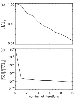
times, they bought only slight improvements to the result of the inversion, and therefore these results are not shown here. Figure 8a shows the reduction of the cost function J (x) as INVICAT performs 10 minimisation iterations relative to its initial value J1. Figure 8b displays the development of

the normalised cost function gradient norm, |∇J (x)|/|∇J1|,

where ∇xJ1 is the initial value of the gradient of the cost

function. J (x) decreases steadily throughout the run, reach-ing a value almost 2 orders of magnitude less than its initial value by the end of the minimisation, whilst the cost function gradient norm is 8 orders of magnitude lower than its initial value after 10 iterations. The contribution of the background term to the total cost function is negligible (not shown), and therefore the value of the observational term decreases by around 99 % during the inversion. The fact that the cost func-tion is reduced so quickly indicates that the minimisafunc-tion program is, at least in this idealised case, working efficiently. Figure 9a shows the difference between the a priori fluxes, xb, and the “true” fluxes xtr, while Fig. 9b shows the differ-ence between the updated a posteriori fluxes after 10 min-imisation iterations, xout, and xtr. The true fluxes have been almost completely retrieved in all grid cells, with only two grid cells still having errors larger than 0.25 kg SF6s−1. The

RMSE of a flux vector x, RMSEx, is defined as

RMSEx= q

(x − xtr₎2_{. (15)}

The RMSE of the a priori emissions, RMSE_xb, is equal to 0.1 kg s−1, while RMSExout is equal to 0.02 kg s−1, mean-ing that approximately 80 % of the total error in the a priori

J/J

1

| J|/| J

|

Fig. 8. (a) Normalised cost function reduction for INVICAT retrieval using pseudoSF6observations.

(b) Normalised cost function gradient development for the same experiment.

42

(a)

(b)

Figure 8. (a) Normalised cost function reduction for INVICAT

re-trieval using pseudo SF6observations. (b) Normalised cost function

gradient development for the same experiment.

emissions have been corrected by INVICAT. It should be noted that the test described here does not include any ran-dom error term being ascribed to the observations, which would be a significant issue for future inversions using real data. This test should therefore not been seen to be represen-tative of the performance of INVICAT in a real application, but as an assessment of the capability of ATOMCAT and the minimisation program to retrieve a known set of emissions.

An important step in the development of our variational system is finding a way to measure the error reduction achieved by an inversion. The variational inverse method does not allow for explicit output of the a posteriori error covariance matrix, and therefore must be approximated from the variables which can be produced during the inversion. For experiments such as the one described in this section, which use the forward model to produce pseudo-observations that are consistent with the error covariance matrices, an ensem-ble of observations can be carried out in order to measure the robustness of the result, as in Chevallier et al. (2007). For inversions which assimilate genuine observations of trace gases, meanwhile, it is possible to output the leading eigen-vectors and eigenvalues of the Hessian of J (x) as a by-product of the inversion, which can be used to approximate the posterior error covariance matrix as shown in Chevallier et al. (2005) and Meirink et al. (2008b). It is our aim to de-velop this technique within INVICAT, allowing us to quan-tify the error reduction of a given inversion.

a

b

kg SF s

-1

Fig. 9. (a) A priori flux error (kggridcell−1_s−1_{) for INVICAT experiment using pseudo-observations,}

defined as xb− xtr, where xbis the a priori flux estimate and is created by randomly perturbating the

“true” fluxes, xtrconsistently with the error statistics of the a priori. (b) A posteriori flux error for the

same experiment after 10 minimisation iterations, defined as x10− xtr.

43

Figure 9. (a) A priori flux error (kg grid cell−1s−1) for INVICAT experiment using pseudo-observations, defined as xb−xtr, where

xbis the a priori flux estimate and is created by randomly perturbing the “true” fluxes, xtr, consistently with the error statistics of the a priori. (b) A posteriori flux error for the same experiment after 10 minimisation iterations, defined as xout−xtr.

The scenario described in this experiment is clearly ide-alised, as it serves to test the capabilities of the inverse model in the most optimal conditions. The cost function is converg-ing towards a minimum, with a relatively small number of iterations, and is reproducing xtrwith high level of accuracy. This indicates that the performance of INVICAT is currently robust enough to allow us to carry out inversions with gen-uine observational data.

7 Summary

We have presented thorough details of the development and testing of an adjoint version of the transport section of the TOMCAT CTM and a variational inverse model for the pur-pose of updating surface fluxes through data assimilation. These models are named ATOMCAT and INVICAT, respec-tively, and are initially intended to analyse the carbon and methane cycles using observed atmospheric concentration data from in situ measurements and remote sensing. The ad-joint model was coded by hand, without the use of auto-matic differentiation tools, for transport subroutines repre-senting advection in three separate directions, convection and boundary layer mixing. In each case, the discrete adjoint of each subroutine was created directly from the original TOM-CAT code, rather than developing a continuous adjoint from the equations governing the transport in the forward model. Meanwhile, since the adjoint model depends upon the state of the forward model at each time step, the forward TOMCAT model was updated in order to save the necessary informa-tion so that they may be read by ATOMCAT.

We investigated the accuracy of the transport scheme in-cluded in the TOMCAT model using the atmospheric trace gas SF6. TOMCAT had previously been included in the

TransCom CH4 model intercomparison, where it had

per-formed accurately in comparison both with observations and with other transport models for SF6. Further tests showed

that TOMCAT captures the seasonality of atmospheric trans-port well at surface stations, and that reducing the resolu-tion of the model grid by approximately 50 % did not signif-icantly impact the model transport representation. Initially, it is therefore likely that INVICAT will initially be run using the lower model grid resolution in order to maximise running speed and minimise data storage.

Each individual transport routine contained within the joint model was tested to ensure that they satisfied the ad-joint identity equation, before being combined to form the complete adjoint transport model. This too was tested thor-oughly, using the adjoint identity equation, the property of reciprocity that must hold for adjoint transport, and finally the Taylor expansion of the cost function. The reciprocity condition held up to machine epsilon, for tests involving ev-ery surface grid cell over a time period of 1 day, and also for selected grid cells over a longer time period of 1 month. This level of accuracy, exact up to the accuracy of the ma-chine used to carry out the tests, strongly implies that the adjoint transport model is indeed analogous to the transport in TOMCAT.

Concurrently with the development of INVICAT and ATOMCAT, a group at the University College London have developed an alternative adjoint version of the TOMCAT model (RETRO-TOM) (Haines et al., 2014). This takes ad-vantage of the property of time symmetry held by the Prather advection scheme by using an Eulerian backtracking method to find adjoint sensitivities. Due to the differing philosophies behind RETRO-TOM and ATOMCAT, each adjoint model has its own distinct advantages. RETRO-TOM does not re-quire output from a forward model simulation, and so is cur-rently likely to be better suited as an alternative to Lagrangian backtracking (e.g. Haines and Esler, 2014). This also means that RETRO-TOM can easily be run using different model grid resolutions. However, ATOMCAT has the advantage that it is not reliant upon its component transport routines being time symmetric, which allows greater freedom of choice than for RETRO-TOM. RETRO-TOM is not currently coupled to a data assimilation of inverse modelling framework, but it would be an interesting avenue of further study to explore the possibility of including RETRO-TOM as an option for adjoint transport within INVICAT. Examining differences in the performances of the two models would allow us to pro-duce the most accurate and consistent inversion results.

Finally, the ability of the variational system INVICAT, which incorporates ATOMCAT, to update surface fluxes through data assimilation was investigated using pseudo “ob-servations” produced using TOMCAT. The model was able to reproduce a set of surface fluxes from a perturbed a pri-ori very closely, reducing the cost function by approximately two orders of magnitude within ten minimisation iterations. The model will now be applied to studies of CH4and CO2,

assimilating real observations from both in situ measure-ments and remote sensing instrumeasure-ments. However, real inverse modelling studies would require investigation into the opti-mal values of the error covariance matrices R and B, which is discussed further in Singh et al. (2011) and Berchet et al. (2013).

Code availability

TOMCAT/SLIMCAT (www.see.leeds.ac.uk/tomcat) is a UK community model. It is available to UK (or NERC-funded) researchers who normally access the model on common fa-cilities or who are helped to install it on their local machines. As it is a complex research tool, new users will need help to use the model optimally. We do not have the resources to release and support the model in an open way. Any potential user interested in the model should contact Martyn Chipper-field.

The model updates described in this paper (INVICAT and ATOMCAT) will be included in the standard model library in the future and therefore will be similarly available only to those who are able to support TOMCAT. The minimisa-tion code M1QN3, meanwhile, is protected by copyright and cannot be distributed except with the permission of its au-thors. For the review process a limited version of the INVI-CAT code was made available to the editors, which included sections of the ATOMCAT and TOMCAT code. This code formed the basis of that used to carry out the accuracy exper-iments described in Sect. 6.1. Inquiries into the availability of the ATOMCAT/INVICAT code can be addressed to the authors.

Acknowledgements. This work was supported by funding from

NERC and NCEO. The TOMCAT model is also supported by NCAS. Manuel Gloor was financially supported by the NERC Consortium grant AMAZONICA (NE/F005806/1) and the EU 7th Framework GEOCARBON project (grant no. agreement 283080), Chris Wilson by a NERC DARC studentship and the NERC consortium grant GAUGE. The authors are grateful for data obtained from the World Data Centre of Greenhouse Gases, provided by NOAA/ESRL. The minimisation pro-gram M1QN3 is part of the MODULOPT library at INRIA (https://who.rocq.inria.fr/Jean-Charles.Gilbert/modulopt/), and the authors thank the company for its permission to use the minimiser. We also thank Wuhu Feng (NCAS).

Edited by: A. Sandu

References

Amsallem, D., Zahr, M., Choi, Y., and Farhat, C.: Design Opti-mization Using Hyper-Reduced-Order Models, Technical report, Stanford University, 2013.

Andersson, E., Fisher, M., Munro, R., and McNally, A.: Diagnosis of background errors for radiances and other observable quanti-ties in a variational data assimilation scheme, and the