HAL Id: hal-01996639
https://hal-univ-tlse2.archives-ouvertes.fr/hal-01996639
Submitted on 28 Jan 2019
HAL is a multi-disciplinary open access
archive for the deposit and dissemination of
sci-entific research documents, whether they are
pub-lished or not. The documents may come from
teaching and research institutions in France or
abroad, or from public or private research centers.
L’archive ouverte pluridisciplinaire HAL, est
destinée au dépôt et à la diffusion de documents
scientifiques de niveau recherche, publiés ou non,
émanant des établissements d’enseignement et de
recherche français ou étrangers, des laboratoires
publics ou privés.
Distributed under a Creative Commons Attribution| 4.0 International License
Holocene Hydroclimate Variability in Central
Scandinavia Inferred from Flood Layers in Contourite
Drift Deposits in Lake Storsjön
Inga Labuhn, Dan Hammarlund, Emmanuel Chapron, Markus Czymzik,
Jean-Pascal Dumoulin, Andreas Nilsson, Édouard Régnier, Joakim Robygd,
Ulrich von Grafenstein
To cite this version:
Inga Labuhn, Dan Hammarlund, Emmanuel Chapron, Markus Czymzik, Jean-Pascal Dumoulin, et al..
Holocene Hydroclimate Variability in Central Scandinavia Inferred from Flood Layers in Contourite
Drift Deposits in Lake Storsjön. Quaternary, MDPI, 2018, 1 (1), pp.1-24. �10.3390/quat1010002�.
�hal-01996639�
Article
Holocene Hydroclimate Variability in Central
Scandinavia Inferred from Flood Layers in Contourite
Drift Deposits in Lake Storsjön
Inga Labuhn1,*, Dan Hammarlund1ID, Emmanuel Chapron2, Markus Czymzik1,3, Jean-Pascal Dumoulin4, Andreas Nilsson1, Edouard Régnier5, Joakim Robygd1
and Ulrich von Grafenstein5
1 Department of Geology, Lund University, Sölvegatan 12, 223 62 Lund, Sweden;
dan.hammarlund@geol.lu.se (D.H.); andreas.nilsson@geol.lu.se (A.N.); j.robygd@gmail.com (J.R.) 2 Laboratoire GEODE, UMR 5602 CNRS-Université Toulouse Jean Jaurès, Maison de la Recherche,
5 Allée Antonio Machado, 31058 Toulouse, France; emmanuel.chapron@univ-tlse2.fr
3 Leibniz Institute for Baltic Sea Research (IOW), Marine Geology, 18119 Rostock-Warnemünde, Germany; czymzik@io-warnemuende.de
4 Laboratoire de Mesure du Carbone 14 (LMC14), LSCE/IPSL, CEA-CNRS-UVSQ, Université Paris-Saclay, 91191 Gif-sur-Yvette, France; jean-pascal.dumoulin@lsce.ipsl.fr
5 Laboratoire des Sciences du Climat et de l’Environnement (LSCE/IPSL), UMR 8212 (CEA/CNRS/UVSQ), Université Paris-Saclay, 91191 Gif-sur-Yvette, France; edouard.regnier@lsce.ipsl.fr (E.R.);
uli@von-grafenstein.fr (U.v.G.)
* Correspondence: inga.labuhn@geol.lu.se; Tel.: +46-46-222-3955
Received: 4 December 2017; Accepted: 28 January 2018; Published: 6 February 2018
Abstract:Despite the societal importance of extreme hydroclimate events, few palaeoenvironmental studies of Scandinavian lake sediments have investigated flood occurrences. Here we present a flood history based on lithological, geochemical and mineral magnetic records of a Holocene sediment sequence collected from contourite drift deposits in Lake Storsjön (63.12◦ N, 14.37◦E). After the last deglaciation, the lake began to form around 9800 cal yr BP, but glacial activity persisted in the catchment for ~250 years. Element concentrations and mineral magnetic properties of the sediments indicate relatively stable sedimentation conditions during the Holocene. However, human impact in the form of expanding agriculture is evident from about 1100 cal yr BP, and intensified in the 20th century. Black layers containing iron sulphide appear irregularly throughout the sequence. The increased influx of organic matter during flood events led to decomposition and oxygen consumption, and eventually to anoxic conditions in the interstitial water preserving these layers. Elevated frequencies of black layer occurrence between 3600 and 1800 cal yr BP reflect vegetation changes in the catchment as well as large-scale climatic change. Soil erosion during snowmelt flood events increased with a tree line descent since the onset of the neoglacial period (~4000 cal yr BP). The peak in black layer occurrence coincides with a prominent solar minimum ~2600 cal yr BP, which may have accentuated the observed pattern due to the prevalence of a negative NAO index, a longer snow accumulation period and consequently stronger snowmelt floods.
Keywords: lake sediments; palaeo-floods; hydroclimate; deglaciation; black layers; contourite; seismic profile; X-ray fluorescence; environmental magnetism; Holocene; Sweden
1. Introduction
Numerous Holocene palaeoclimate studies have been performed in Scandinavia, many of which are based on lake sediment records [1–7]. The Scandes Mountains are particularly important for our understanding of climate variations in this region through their wealth of suitable sites along ecological
Quaternary 2018, 1, 2 2 of 24
gradients and their proximity to the climatically dynamic North Atlantic region [8–14]. However, previous studies have almost exclusively investigated sediments deposited in small and relatively shallow lakes, predominantly reflecting local-scale environmental dynamics. In contrast, sediment archives from large lakes with more extensive watersheds integrate across regional hydroclimate regimes, although their responses to environmental changes may be subdued due to longer water residence times and relatively insensitive biota [6,15]. A number of large and deep lakes are located on the lee side of the Scandes Mountains. Close to 20 of these lakes, which were formed by glacial scouring during repeated glaciations, exceed 100 km2in areal extent and many are >100 m deep. However, sediment records from this type of lake have remained largely unexplored as palaeoclimate archives in Scandinavia, although they have played an important role in the development of highly resolved records of Holocene climate change in continental Europe and other parts of the world [16–19]. In addition, the majority of previously published climate reconstructions from Scandinavia have focused primarily on temperature, while variations in hydroclimate, both gradual changes and extreme events like floods, have been partly overlooked, in spite of their societal importance [20].
Flood occurrences are non-stationary through time and the main driver of their frequency and intensity is the internal and external climate forcing on inter-annual to millennial time-scales [21–25]. However, our knowledge of flood occurrences in Scandinavia is limited due to the general lack of long palaeoclimate records reflecting such extreme events. Reconstructions of past flood occurrences would allow us to better understand their return period as a response to varying climate forcing [26–29] and may improve the anticipation of future flood risks.
During a flood, fine-grained detrital material is eroded in the catchment and transported in suspension into downstream lakes. When the transport capacity of the inflowing tributary stream diminishes in the water body, the terrigenous material is transported through hypo-, meso-, homo- or hyperpycnal flows and is finally deposited as a distinct detrital flood layer on the lake floor [30,31]. Detrital layers have been explored to reconstruct flood occurrences, but such studies are essentially limited to smaller lakes or sites in the vicinity of tributary rivers [25,26,28,32]. For larger lakes, currents associated with flood events or linked to specific wind regimes can modify the distribution of flood layers [33–40]. Hyperpycnal flows during flood events are strongly controlled by and tend to maintain, the lake floor morphology (i.e., channels). They can export sediment plumes containing river suspended load far away from the delta into deep basins. Lacustrine contourite deposits have been described in lakes with different basin shapes, depths and circulations patterns, e.g., in Lake Superior [41], East African Lakes [42], Lake Baikal [43], Lake Geneva [35] and Patagonian Lakes [38]. These drift deposits are either resulting from the influence of the Coriolis force on the displacement of sediment plumes at the lake floor, and/or from the interaction of hyperpycnal flood events (or turbidity currents) with currents at the lake floor generated by wind-induced internal waves or gyres. Here we present a 4 m thick Holocene sediment sequence from contourite deposits in Lake Storsjön, a large lake on the lee-side of the Scandes Mountains in central Sweden. A particular focus is placed on black layers irregularly intercalated into the background deposition of grey, clay-rich sediments and their potential to serve as a proxy for past changes in the frequency of strong snowmelt floods. In addition, an ensemble of lithological, chemical and mineral magnetic proxies is used to reconstruct variations in catchment dynamics and in-lake processes, providing new insights into the deglaciation history of the site, millennial-scale climatic and environmental changes in the region during the Holocene and human impact on sediment deposition during recent centuries. Based on this multi-proxy approach, we investigate to what extent proxy variability in the sediments of Lake Storsjön relates to large-scale Holocene climate dynamics in Scandinavia.
2. Materials and Methods
2.1. Study Area
Lake Storsjön is located in central Sweden (63.12◦ N, 14.37◦ E; Figure 1a). Average annual temperature at the Frösön meteorological station, located on an island in the lake, is 2.5◦C, with average monthly temperatures ranging from −8.6 ◦C in January to 13.4 ◦C in July. The average annual precipitation is 491 mm, with >50% falling between June and September (Figure1b; all values refer to the 1960–1990 reference period). The surrounding bedrock is mainly composed of greywackes, shales and limestones of Cambro-Silurian age, partly altered by the Caledonian orogeny, covered by a Quaternary clayey diamicton [44]. The catchment area of about 12,000 km2extends from the water divide of the Scandes Mountains at a maximum elevation of 1796 m to the outlet of the lake at 292 m a.s.l. (Figure1c). It is dominated by coniferous forest (40%) and mires, with some cultivated areas on the clay-rich soils on carbonate bedrock. Lake Storsjön itself covers an area of 456 km2, with 13% of the
catchment area consisting of lakes.
Quaternary 2018, 1, 2 3 of 24
2. Materials and Methods
2.1. Study Area
Lake Storsjön is located in central Sweden (63.12° N, 14.37° E; Figure 1a). Average annual temperature at the Frösön meteorological station, located on an island in the lake, is 2.5 °C, with average monthly temperatures ranging from −8.6 °C in January to 13.4 °C in July. The average annual precipitation is 491 mm, with >50% falling between June and September (Figure 1b; all values refer to the 1960–1990 reference period). The surrounding bedrock is mainly composed of greywackes, shales and limestones of Cambro‐Silurian age, partly altered by the Caledonian orogeny, covered by a Quaternary clayey diamicton [44]. The catchment area of about 12,000 km2 extends from the water divide of the Scandes Mountains at a maximum elevation of 1796 m to the outlet of the lake at 292 m a.s.l. (Figure 1c). It is dominated by coniferous forest (40%) and mires, with some cultivated areas on the clay‐rich soils on carbonate bedrock. Lake Storsjön itself covers an area of 456 km2, with 13% of the catchment area consisting of lakes. Figure 1. (a) Overview map showing the location of the study area; (b) Climate diagram for the Frösön meteorological station (1961–1990 averages); (c) The catchment of Lake Storsjön (dark grey shading); (d) Bathymetry of Lake Storsjön, position of the coring site (black dot), location of the Frösön meteorological station (black star) and the seismic profiles (black lines). A, B, C, D and E indicate the subdivision of the lake into five principal parts (see text for details). The lake has a mean depth of 17.3 m, a maximum depth of 74 m and a volume of 8.02 km3. It can be divided into five principal parts (A to E; Figure 1d) according to its bathymetry and exposure to inlets and to the outlet. Due to the large catchment compared to the size of the lake, its water residence time of about 1 year is relatively short, with a more rapid throughflow in the northern parts of the lake, where the in‐ and outflows are located and a longer residence time in its southern basins [45]. The average ice cover period of Lake Storsjön lasts from mid‐December to mid‐May. Snowmelt leads to a distinct peak in river discharge in the catchment in May or June [46]. However, river management at >10 hydropower stations upstream of Storsjön’s main inlet masks the natural seasonal discharge pattern at the inlet. The lake has been regulated by a dam for hydropower production since 1938, involving yearly water level variations in the range of 290.5–293.3 m a.s.l. The development of a thermocline at 17–26 m water depth has been recorded in September in several parts (B, C and E) on a number of occasions between 2010 and 2014 [45]. Hydrodynamic simulations revealed significant surface currents associated with prevailing wind patterns during the ice‐free season and distinct deeper currents linked to the lake floor morphology [45].
Figure 1. (a) Overview map showing the location of the study area; (b) Climate diagram for the Frösön meteorological station (1961–1990 averages); (c) The catchment of Lake Storsjön (dark grey shading); (d) Bathymetry of Lake Storsjön, position of the coring site (black dot), location of the Frösön meteorological station (black star) and the seismic profiles (black lines). A, B, C, D and E indicate the subdivision of the lake into five principal parts (see text for details).
The lake has a mean depth of 17.3 m, a maximum depth of 74 m and a volume of 8.02 km3. It can be divided into five principal parts (A to E; Figure1d) according to its bathymetry and exposure to inlets and to the outlet. Due to the large catchment compared to the size of the lake, its water residence time of about 1 year is relatively short, with a more rapid throughflow in the northern parts of the lake, where the in- and outflows are located and a longer residence time in its southern basins [45].
The average ice cover period of Lake Storsjön lasts from mid-December to mid-May. Snowmelt leads to a distinct peak in river discharge in the catchment in May or June [46]. However, river management at >10 hydropower stations upstream of Storsjön’s main inlet masks the natural seasonal discharge pattern at the inlet. The lake has been regulated by a dam for hydropower production since 1938, involving yearly water level variations in the range of 290.5–293.3 m a.s.l. The development of a thermocline at 17–26 m water depth has been recorded in September in several parts (B, C and E) on a number of occasions between 2010 and 2014 [45]. Hydrodynamic simulations revealed significant surface currents associated with prevailing wind patterns during the ice-free season and distinct deeper currents linked to the lake floor morphology [45].
Quaternary 2018, 1, 2 4 of 24
2.2. Seismic Survey
A seismic survey using a portable 4 kHz chirp digital device (Knudsen; Perth, Canada) and a conventional GPS (Garmin, Olathe, KS, USA) installed on-board a small fishing boat was performed during three days in November 2013 for mapping of the bedrock morphology and sediment geometry, as well as for identification of suitable coring sites. In total, 90 km of seismic profiles were acquired based on available bathymetric data [45], essentially in parts C and E of the lake, while strong winds and large waves prevented surveying the central basin.
2.3. Sediment Coring
Sediment cores were retrieved from the ice-covered lake in April 2014 in a 33 m deep basin with no major inlets in its vicinity. The seismic data at this location indicated a high sediment thickness and an undisturbed stratigraphy (Figures2and3). An 86 cm long surface sediment core was obtained using a freeze corer [47]. Seven overlapping 2 m long sediment cores, 8.3 cm in diameter, were obtained from three adjacent drill holes using a UWITEC piston corer (Mondsee, Austria).
Quaternary 2018, 1, 2 4 of 24
2.2. Seismic Survey
A seismic survey using a portable 4 kHz chirp digital device (Knudsen; Perth, Canada) and a conventional GPS (Garmin, Olathe, KS, USA) installed on‐board a small fishing boat was performed during three days in November 2013 for mapping of the bedrock morphology and sediment geometry, as well as for identification of suitable coring sites. In total, 90 km of seismic profiles were acquired based on available bathymetric data [45], essentially in parts C and E of the lake, while strong winds and large waves prevented surveying the central basin.
2.3. Sediment Coring
Sediment cores were retrieved from the ice‐covered lake in April 2014 in a 33 m deep basin with no major inlets in its vicinity. The seismic data at this location indicated a high sediment thickness and an undisturbed stratigraphy (Figures 2 and 3). An 86 cm long surface sediment core was obtained using a freeze corer [47]. Seven overlapping 2 m long sediment cores, 8.3 cm in diameter, were obtained from three adjacent drill holes using a UWITEC piston corer (Mondsee, Austria).
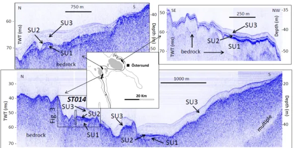
Figure 2. Selected examples of acoustic facies identified on seismic profiles (bold black lines on the map), highlighting the complex morphology of the bedrock and variable successions of seismic units (SU1, SU2 and SU3) across the lake basin. The locations of the coring site (STO14) and Figure 3 are indicated on the bottom panel.
Figure 3. Detail of a seismic profile indicating the correlation of acoustic facies and sedimentary facies
from the STO14 sediment sequence as described in supplementary Figure S1. The location of this profile is indicated in Figure 2.
Figure 2.Selected examples of acoustic facies identified on seismic profiles (bold black lines on the map), highlighting the complex morphology of the bedrock and variable successions of seismic units (SU1, SU2 and SU3) across the lake basin. The locations of the coring site (STO14) and Figure3are indicated on the bottom panel.
Quaternary 2018, 1, 2 4 of 24
2.2. Seismic Survey
A seismic survey using a portable 4 kHz chirp digital device (Knudsen; Perth, Canada) and a conventional GPS (Garmin, Olathe, KS, USA) installed on‐board a small fishing boat was performed during three days in November 2013 for mapping of the bedrock morphology and sediment geometry, as well as for identification of suitable coring sites. In total, 90 km of seismic profiles were acquired based on available bathymetric data [45], essentially in parts C and E of the lake, while strong winds and large waves prevented surveying the central basin.
2.3. Sediment Coring
Sediment cores were retrieved from the ice‐covered lake in April 2014 in a 33 m deep basin with no major inlets in its vicinity. The seismic data at this location indicated a high sediment thickness and an undisturbed stratigraphy (Figures 2 and 3). An 86 cm long surface sediment core was obtained using a freeze corer [47]. Seven overlapping 2 m long sediment cores, 8.3 cm in diameter, were obtained from three adjacent drill holes using a UWITEC piston corer (Mondsee, Austria).
Figure 2. Selected examples of acoustic facies identified on seismic profiles (bold black lines on the map), highlighting the complex morphology of the bedrock and variable successions of seismic units (SU1, SU2 and SU3) across the lake basin. The locations of the coring site (STO14) and Figure 3 are indicated on the bottom panel.
Figure 3. Detail of a seismic profile indicating the correlation of acoustic facies and sedimentary facies
from the STO14 sediment sequence as described in supplementary Figure S1. The location of this profile is indicated in Figure 2.
Figure 3.Detail of a seismic profile indicating the correlation of acoustic facies and sedimentary facies from the STO14 sediment sequence as described in supplementary Figure S1. The location of this profile is indicated in Figure2.
2.4. Core Correlation
A continuous composite sediment profile of 7 m thickness (STO14) was constructed from the freeze core and the piston cores (supplementary material, Figure S1). The overlapping parts of the piston cores were aligned using 19 macroscopic lithological marker layers. Two of the cores were aligned at 440 cm based on their coring depths due to absence of clear stratigraphic markers. The freeze core was connected to the uppermost piston core based on six tie points identified in organic matter contents and element concentrations obtained from loss on ignition (LOI) and X-ray fluorescence (XRF) measurements, respectively (see below).
2.5. Dating and Age Modelling
Seven terrestrial macroscopic plant remains were identified under a binocular microscope and used for AMS radiocarbon dating at the LMC14 laboratory in Saclay (France) [48–50] and at the Radiocarbon Dating Laboratory at Lund University, Sweden (Table1). Measured radiocarbon ages were calibrated using the IntCal13 calibration dataset [51] and are expressed as calibrated years before 1950 CE (cal yr BP).
Marker horizons of pollution lead were identified using Pb concentrations determined by XRF (see below). Enrichment factors of Pb were calculated relative to a conservative lithogenic element (Zr) and a background value of Pb according to [52]. A site-specific Pb background was calculated using the part of the sediment sequence deposited prior to 2500 cal yr BP, i.e., before the earliest Pb pollution signals [53]. The anthropogenic Pb contribution was then calculated following [54]. An age uncertainty of±50 years was assigned to the inferred Pb pollution dates to account for the sampling resolution of 0.5 to 1 cm.
Activities of210Pb and137Cs were measured on the upper 21 cm of the freeze core with an ORTEC High-Purity Germanium Gamma Detector (AMETEK Inc., Berwin, PA, USA) at the Department of Geology, Lund University. The 210Pb activity was measured at its gamma peak at 46.5 KeV, the224Ra was determined via its granddaughters114Pb at 295 KeV and 352 KeV and114Bi at 609 KeV. Self-absorption corrections were made for210Pb on each measurement [55]. The137Cs activity was measured at the 662 KeV gamma peak.
The age-depth model for the sediment sequence was created with Clam version 2.2 [56] using a smoothing spline with a smooth level of 0.3, including seven14C dates, three pollution Pb dates and one137Cs date (210Pb dating was not possible due to insufficient sample sizes). The sampling year 2014 (−64 cal yr BP) was assigned to the top of the composite profile.
2.6. Sediment Subsampling
The sediment sequence was subsampled for lithological, chemical and mineral magnetic analyses. A continuous series of sediment samples was extracted from the freeze core at 1 cm resolution from 1.5 to 10.5 cm depth (top sample 0–1.5 cm), at 0.5 cm resolution from 10.5 to 20 cm depth and at 1 cm resolution from 20 to 81 cm depth. The piston cores were sampled using cubic boxes (7 cm3) at 3 cm resolution, with the topmost sample centred at 1.5 cm depth. In addition to the regular interval samples, 14 samples were extracted from individual black layers, with a thickness between 0.4 and 0.7 cm.
2.7. Physical and Chemical Properties
Grey level values were extracted from a digital greyscale photograph (resolution 300 dpi) of the sediment sequence, along the vertical axis and averaged over a 2 cm wide horizontal window. Grey level values are expressed on a scale between 0 (black) and 255 (white).
Grain size distributions were determined for six black layers and six regular sediment (clay gyttja) samples of about 2.5 g dry weight. Samples were sieved with 250, 125 and 63 µm mesh sizes and each fraction was weighed with a precision balance. Three of the black layers and three of the clay
Quaternary 2018, 1, 2 6 of 24
gyttja samples were inspected at 15 kV with a Hitachi S-3400N (Tokyo, Japan) scanning electron microscope (SEM) at the Department of Geology, Lund University.
XRF and LOI were measured on the regular interval samples throughout the sequence and on the 14 black layer samples. XRF was measured using a Thermo Scientific Niton XL3t Goldd+ XRF analyser (ThermoFisher Scientific Inc., Waltham, MA, USA) in mining mode (Cu/Zn) for 180 s. All measurements were duplicated and the presented values are averages of the replicate measurements. Water and organic matter contents were determined by LOI using a Nabertherm muffle furnace (Lilienthal, Germany), following [57]. Samples were first heated to 105◦C for two hours and then combusted at 550◦C for four hours. The samples were weighed before and after each step. 2.8. Mineral Magnetic Properties
Mineral magnetic measurements were carried out on the regular interval samples at the Lund Paleomagnetic Laboratory. A first set of samples covering the composite sediment sequence was measured in September 2014 and a second set, comprising the overlapping parts of the piston cores, was measured in August 2016. Volume-specific magnetic susceptibilities (κ) were measured on all samples using a Geofyzica Brno KLY-2 kappabridge (Brno, Czech Republic). Anhysteretic remanent magnetizations (ARMs) were induced with a peak alternating field (AF) of 80mT with a direct current (DC) bias field of 50µT and progressively AF demagnetized at 5, 10, 15, 20, 40, 60 and 80 mT. Volume-specific susceptibility of ARM (κARM) was calculated by normalizing the ARM
intensity by the DC bias field and median destructive field of the ARM (MDFARM) determined as the
AF required to remove 50% of the induced ARM. ARM measurements were not carried out for samples collected from the freeze core. Saturation isothermal remanent magnetizations (SIRMs) were induced using a Redcliffe model BSM-700 pulse magnetizer (Redcliffe Magtronics Ltd., Bristol, UK) with a DC field of 1T and measured using a Molspin Minispin magnetometer. Backfield IRMs were subsequently induced with a DC field of 100mT using a Molspin pulse magnetizer and measured using a Molspin Minispin magnetometer (Bartington Instruments Ltd., Witney, UK). S-ratios were determined by dividing the backfield IRM-100mTwith the SIRM. After completion of the magnetic measurements,
the samples from the composite sequence were freeze dried in order to calculate dry density.
3. Results
3.1. Seismic Survey
Seismic profiles allowed mapping of the bedrock morphology corresponding to the acoustic substratum (Figures2and3). The complex morphology of the bedrock is typical for lakes of glacial origin, showing numerous over-deepened sub-basins delimited by sills or islands [58]. The bedrock crops out frequently at the lake floor (Figure2) and is covered by unevenly distributed sediments constituting a succession of seismic units with contrasting acoustic facies. Seismic Unit 1 (SU1) is characterized by a varying thickness across the studied parts of the lake basin, ranging from 0 to 10 milliseconds two-way travel time (ms TWT) and consisting of transparent to chaotic acoustic facies with local high amplitude and continuous reflections (Figure2). SU1 exhibits maximum thickness in Part C. Seismic Unit 2 (SU2) is characterized by a continuous and high-amplitude reflection and is generally thin (<1 ms TWT). In contrast, Seismic Unit 3 (SU3) is characterized by transparent acoustic facies (<10 ms TWT thick) and by the development of several low amplitude continuous reflections parallel to the lake floor that are locally developing onlap terminations on SU2, SU1 or the bedrock (Figures2and3). In addition, SU3 displays a channel-levee configuration typical of (patchy) drift or contourite deposits.
3.2. Lithological Description
Three main lithological units (I, II and III) were identified in the sediment sequence (Figure S1). These sedimentary units correspond to the seismic units (SU) identified in 0: Unit I corresponds to SU1,
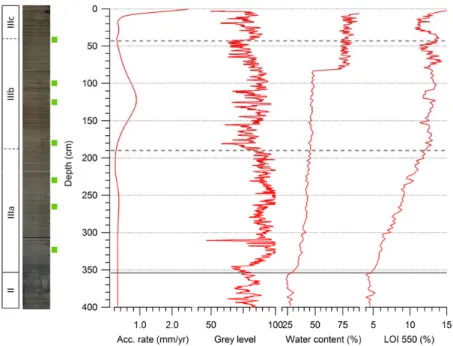
Unit II to SU2 and Unit III to SU3 (Figure3). Unit I (715–399 cm depth) consists of dark grey, poorly sorted, sandy-silty diamictic sediments with abundant gravel and small stones (Subunits Ia, Ib and Id), interrupted by layers of predominantly clayey-silty sediments at two levels (Subunits Ic and Ie). Unit II (399–354 cm) is sharply distinguished from Unit I and is composed of finely laminated couplets of dark and light grey clay, with thicknesses between 1 and 2 mm. Unit III (354–0 cm) consists of brownish grey clay gyttja with occasional macroscopic terrestrial plant remains. Throughout Unit III, 335 black layers of 0.1 to 0.7 cm thickness appear at intervals between 0.2 and 3.5 cm (Figure4). After the core opening, their colour changed gradually into reddish-brown. Vivianite concretions around macroscopic plant remains were identified visually (based on the bright blue colour upon exposure to air) within black layers at 153.5, 171, 180.5, 231 and 230 cm depth. Unit III is subdivided into three parts (Figure5). Subunit IIIa (354–190 cm) is of grey colour and shows a steadily increasing organic matter content. Above 190 cm depth the sediment colour changes gradually from grey to brown, illustrated also by a decrease in grey level value (Figure5) and the organic matter content remains relatively stable (Subunit IIIb). Subunit IIIc (43–0 cm) is defined by the onset of increasing concentrations in several elements (see below). Only Units II and III were analysed in detail for this study, as Unit I does not represent lacustrine sediments and lacks chronological information (see Section4.1).
Quaternary 2018, 1, 2 7 of 24
couplets of dark and light grey clay, with thicknesses between 1 and 2 mm. Unit III (354–0 cm) consists of brownish grey clay gyttja with occasional macroscopic terrestrial plant remains. Throughout Unit III, 335 black layers of 0.1 to 0.7 cm thickness appear at intervals between 0.2 and 3.5 cm (Figure 4). After the core opening, their colour changed gradually into reddish‐brown. Vivianite concretions around macroscopic plant remains were identified visually (based on the bright blue colour upon exposure to air) within black layers at 153.5, 171, 180.5, 231 and 230 cm depth. Unit III is subdivided into three parts (Figure 5). Subunit IIIa (354–190 cm) is of grey colour and shows a steadily increasing organic matter content. Above 190 cm depth the sediment colour changes gradually from grey to brown, illustrated also by a decrease in grey level value (Figure 5) and the organic matter content remains relatively stable (Subunit IIIb). Subunit IIIc (43–0 cm) is defined by the onset of increasing concentrations in several elements (see below). Only Units II and III were analysed in detail for this study, as Unit I does not represent lacustrine sediments and lacks chronological information (see Section 4.1).
Figure 4. Close‐up photograph of the STO14 sediment sequence (Unit III, 28 to 36.5 cm depth)
showing the background sedimentation of brown clay gyttja and the intercalated black layers. The unit on the rule is cm.
Figure 5. Division of lithological units of the STO14 sediment sequence, composite photograph of the
sediments sequence, depths of radiocarbon dates (green squares), accumulation rate, grey level of the photograph, water content and organic matter content (LOI). The abrupt change in water content reflects the different coring techniques (freeze core above 80 cm, piston cores below 80 cm), as there is some water loss from the piston cores during storage and sampling.
Figure 4.Close-up photograph of the STO14 sediment sequence (Unit III, 28 to 36.5 cm depth) showing the background sedimentation of brown clay gyttja and the intercalated black layers. The unit on the rule is cm.
Quaternary 2018, 1, 2 7 of 24
couplets of dark and light grey clay, with thicknesses between 1 and 2 mm. Unit III (354–0 cm) consists of brownish grey clay gyttja with occasional macroscopic terrestrial plant remains. Throughout Unit III, 335 black layers of 0.1 to 0.7 cm thickness appear at intervals between 0.2 and 3.5 cm (Figure 4). After the core opening, their colour changed gradually into reddish‐brown. Vivianite concretions around macroscopic plant remains were identified visually (based on the bright blue colour upon exposure to air) within black layers at 153.5, 171, 180.5, 231 and 230 cm depth. Unit III is subdivided into three parts (Figure 5). Subunit IIIa (354–190 cm) is of grey colour and shows a steadily increasing organic matter content. Above 190 cm depth the sediment colour changes gradually from grey to brown, illustrated also by a decrease in grey level value (Figure 5) and the organic matter content remains relatively stable (Subunit IIIb). Subunit IIIc (43–0 cm) is defined by the onset of increasing concentrations in several elements (see below). Only Units II and III were analysed in detail for this study, as Unit I does not represent lacustrine sediments and lacks chronological information (see Section 4.1).
Figure 4. Close‐up photograph of the STO14 sediment sequence (Unit III, 28 to 36.5 cm depth)
showing the background sedimentation of brown clay gyttja and the intercalated black layers. The unit on the rule is cm.
Figure 5. Division of lithological units of the STO14 sediment sequence, composite photograph of the
sediments sequence, depths of radiocarbon dates (green squares), accumulation rate, grey level of the photograph, water content and organic matter content (LOI). The abrupt change in water content reflects the different coring techniques (freeze core above 80 cm, piston cores below 80 cm), as there is some water loss from the piston cores during storage and sampling.
Figure 5.Division of lithological units of the STO14 sediment sequence, composite photograph of the sediments sequence, depths of radiocarbon dates (green squares), accumulation rate, grey level of the photograph, water content and organic matter content (LOI). The abrupt change in water content reflects the different coring techniques (freeze core above 80 cm, piston cores below 80 cm), as there is some water loss from the piston cores during storage and sampling.
Quaternary 2018, 1, 2 8 of 24
3.3. Age Model and Accumulation Rates
A distinct137Cs peak was observed at 5 cm depth (Figure6a). Peak activities of137Cs in lake sediments originate from nuclear bomb tests in the 1960s and the explosion of the Chernobyl nuclear power plant in 1986 CE [59]. Large parts of the Storsjön catchment were affected by137Cs deposition after the Chernobyl accident [60]. It has been shown that137Cs from the Chernobyl fallout in varved sediment sequences from northern Sweden diffused downward and masked the nuclear bomb test peak [61]. Therefore, the observed137Cs peak in the STO14 sediments likely corresponds to the 1986 CE fallout and its presence indicates a well-preserved sediment surface.
Pb concentration peaks in lake sediments can be linked to well-dated events of anthropogenic Pb emissions and widespread, airborne pollution, e.g., at ca. 750 and 420 cal yr BP due to intensified metallurgy in Europe and around -25 cal yr BP due to the use and subsequent ban of leaded petrol [62,63]. The -25 cal yr BP peak can be clearly identified in the STO14 sequence. Two other Pb peaks are interpreted to reflect the 750 and 420 cal yr BP increases in anthropogenic Pb, which have also been identified in other Swedish lakes [53,64] (Figure6b). Although these Pb peaks are not very distinct in the STO14 sediment sequence, the inferred dates are in good agreement with adjacent14C and137Cs dates.
Quaternary 2018, 1, 2 8 of 24
3.3. Age Model and Accumulation Rates
A distinct 137Cs peak was observed at 5 cm depth (Figure 6a). Peak activities of 137Cs in lake
sediments originate from nuclear bomb tests in the 1960s and the explosion of the Chernobyl nuclear power plant in 1986 CE [59]. Large parts of the Storsjön catchment were affected by 137Cs deposition after the Chernobyl accident [60]. It has been shown that 137Cs from the Chernobyl fallout in varved sediment sequences from northern Sweden diffused downward and masked the nuclear bomb test peak [61]. Therefore, the observed 137Cs peak in the STO14 sediments likely corresponds to the 1986 CE fallout and its presence indicates a well‐preserved sediment surface. Pb concentration peaks in lake sediments can be linked to well‐dated events of anthropogenic Pb emissions and widespread, airborne pollution, e.g. at ca. 750 and 420 cal yr BP due to intensified metallurgy in Europe and around ‒25 cal yr BP due to the use and subsequent ban of leaded petrol [62,63]. The ‒25 cal yr BP peak can be clearly identified in the STO14 sequence. Two other Pb peaks are interpreted to reflect the 750 and 420 cal yr BP increases in anthropogenic Pb, which have also been identified in other Swedish lakes [53,64] (Figure 6b). Although these Pb peaks are not very distinct in the STO14 sediment sequence, the inferred dates are in good agreement with adjacent 14C and 137Cs dates. (a) (b) Figure 6. Chronological markers in the STO14 sediment sequence. (a) 137Cs activity for the upper 20 cm. (b) Calculated anthropogenic Pb concentration (red/orange line) and reference curves from varve‐ dated Swedish lakes (blue lines): Kalven (total Pb) [64]; Kostjärn and Kassjön (anthropogenic Pb) [53]. See text for details on the calculation of the anthropogenic Pb concentration. Note that the STO14 Pb concentration data are plotted on different scales to account for different orders of magnitude. The dashed lines indicate the tie points used to infer the pollution Pb dates included in the age model.
The radiocarbon dates are presented in Table 1. The age model indicates no age reversals or apparent hiatuses (Figure 7). As no plant macrofossils for radiocarbon dating were found below 320 cm depth, the age model was extrapolated below this point. Sediment facies like the finely laminated sediments found in Unit II are commonly interpreted as glaciolacustrine varves in Scandinavian lakes, with couplets of light and dark layers defined as one annual sedimentation cycle reflecting the seasonally varying glaciofluvial discharge in ice‐proximal settings [65,66] (see also Section 4.1). Repeated counts of the dark‐light couplets in Unit II yielded 250 (±5) varves and a mean annual sedimentation of 1.8 mm. Since the radiocarbon‐based age model placed the boundary between Units II and III at 9550 ± 200 cal yr BP, the lower boundary of Unit II is tentatively assigned an age of 9800 ± 205 cal yr BP based on counting of the assumed varves.
Figure 6. Chronological markers in the STO14 sediment sequence. (a)137Cs activity for the upper 20 cm. (b) Calculated anthropogenic Pb concentration (red/orange line) and reference curves from varve-dated Swedish lakes (blue lines): Kalven (total Pb) [64]; Kostjärn and Kassjön (anthropogenic Pb) [53]. See text for details on the calculation of the anthropogenic Pb concentration. Note that the STO14 Pb concentration data are plotted on different scales to account for different orders of magnitude. The dashed lines indicate the tie points used to infer the pollution Pb dates included in the age model.
The radiocarbon dates are presented in Table1. The age model indicates no age reversals or apparent hiatuses (Figure7). As no plant macrofossils for radiocarbon dating were found below 320 cm depth, the age model was extrapolated below this point. Sediment facies like the finely laminated sediments found in Unit II are commonly interpreted as glaciolacustrine varves in Scandinavian lakes, with couplets of light and dark layers defined as one annual sedimentation cycle reflecting the seasonally varying glaciofluvial discharge in ice-proximal settings [65,66] (see also Section4.1). Repeated counts of the dark-light couplets in Unit II yielded 250 (±5) varves and a mean annual sedimentation of 1.8 mm. Since the radiocarbon-based age model placed the boundary between Units
II and III at 9550± 200 cal yr BP, the lower boundary of Unit II is tentatively assigned an age of 9800±205 cal yr BP based on counting of the assumed varves.
Sediment accumulation rates are relatively constant from 9550 to 3500 cal yr BP (on average 0.3 mm/year), with elevated values between 3500 and 1500 cal yr BP (maximum 0.89 mm/year around 2600 cal yr BP). The highest accumulation rates (>2 mm/year) are found in the upper 2 cm of the sediment sequence.
Table 1. Radiocarbon dates from the STO14 sediment sequence. Samples were measured at the Laboratoire de Mesure du Carbone 14 (LMC 14), Université Paris-Saclay, France (Sac) and at the Radiocarbon Dating Laboratory, Lund University, Sweden (Lu).
Depth (cm) Material 14C Age BP±Error Cal. Age BP (2σ Range) Lab. ID
41.6 Wood fragment 1165±30 985–1177 SacA39831
100.4 Twig 2330±30 2213–2431 SacA39833
124.5 Wood fragment 2540±30 2497–2747 SacA39832
180.2 Twig 3410±30 3577–3811 SacA39834
229.8 Wood fragments 4950±35 5603–5740 SacA39836
264.4 Twig 5915±40 6657–6847 SacA39835
322.9 Wood fragment 7785±45 8447–8639 LuS11056
Quaternary 2018, 1, 2 9 of 24
Sediment accumulation rates are relatively constant from 9550 to 3500 cal yr BP (on average 0.3 mm/year), with elevated values between 3500 and 1500 cal yr BP (maximum 0.89 mm/year around 2600 cal yr BP). The highest accumulation rates (>2 mm/year) are found in the upper 2 cm of the sediment sequence.
Table 1. Radiocarbon dates from the STO14 sediment sequence. Samples were measured at the
Laboratoire de Mesure du Carbone 14 (LMC 14), Université Paris‐Saclay, France (Sac) and at the Radiocarbon Dating Laboratory, Lund University, Sweden (Lu).
Depth (cm) Material 14C Age BP ± Error Cal. Age BP (2σ Range) Lab. ID
41.6 Wood fragment 1165 ± 30 985–1177 SacA39831 100.4 Twig 2330 ± 30 2213–2431 SacA39833 124.5 Wood fragment 2540 ± 30 2497–2747 SacA39832 180.2 Twig 3410 ± 30 3577–3811 SacA39834 229.8 Wood fragments 4950 ± 35 5603–5740 SacA39836 264.4 Twig 5915 ± 40 6657–6847 SacA39835 322.9 Wood fragment 7785 ± 45 8447–8639 LuS11056
Figure 7. Age‐depth model for the STO14 sediment sequence based on radiocarbon dates (blue dots), pollution Pb marker horizons (green dots) and the 137Cs activity peak (red dot). The year 2014 was
assigned to the top of the sequence. The model was calculated with Clam version 2.2 [56] using a smooth spline with a smoothing level of 0.3. The red line illustrates the layer counting in Unit II (354– 399 cm), assuming annual layers. The topmost lamina was assigned an age corresponding to the extrapolated 14C age at this depth.
3.4. Chemical Sediment Properties
Organic matter contents are relatively stable around 4.5% throughout Unit II (Figure 5). From the Unit II‐III boundary the organic matter content increases steadily throughout Subunit IIIa to about 12.5% around 4000 cal yr BP. In Subunits IIIb and IIIc organic contents become more variable, fluctuating between 10% and 14% but there is no long‐term trend in these Subunits. The highest organic matter content of 15% is found in the topmost sample (Figure 5).
Concentrations of Ti (Figure 8) and other lithogenic elements (Zr, Rb, K and Al; not shown) display largely similar patterns throughout the sediment sequence, with high values in Unit II (prior to 9500 cal yr BP), a constant decrease throughout Unit IIIa (to about 4000 cal yr BP), low values in Unit IIIb (between 4000 and 1100 cal yr BP) and an increase throughout Unit IIIc (from ca. 1100 cal yr BP to present). The average correlation between the lithogenic elements is 0.90 (p < 0.001) and they are all negatively correlated with organic matter contents (r = –0.82; p < 0.001). Si concentrations are
Figure 7.Age-depth model for the STO14 sediment sequence based on radiocarbon dates (blue dots), pollution Pb marker horizons (green dots) and the137Cs activity peak (red dot). The year 2014 was assigned to the top of the sequence. The model was calculated with Clam version 2.2 [56] using a smooth spline with a smoothing level of 0.3. The red line illustrates the layer counting in Unit II (354–399 cm), assuming annual layers. The topmost lamina was assigned an age corresponding to the extrapolated14C age at this depth.
3.4. Chemical Sediment Properties
Organic matter contents are relatively stable around 4.5% throughout Unit II (Figure5). From the Unit II-III boundary the organic matter content increases steadily throughout Subunit IIIa to about 12.5% around 4000 cal yr BP. In Subunits IIIb and IIIc organic contents become more variable, fluctuating between 10% and 14% but there is no long-term trend in these Subunits. The highest organic matter content of 15% is found in the topmost sample (Figure5).
Concentrations of Ti (Figure8) and other lithogenic elements (Zr, Rb, K and Al; not shown) display largely similar patterns throughout the sediment sequence, with high values in Unit II (prior to 9500 cal yr BP), a constant decrease throughout Unit IIIa (to about 4000 cal yr BP), low values in Unit IIIb
Quaternary 2018, 1, 2 10 of 24
(between 4000 and 1100 cal yr BP) and an increase throughout Unit IIIc (from ca. 1100 cal yr BP to present). The average correlation between the lithogenic elements is 0.90 (p < 0.001) and they are all negatively correlated with organic matter contents (r =−0.82; p < 0.001). Si concentrations are not strongly correlated with the lithogenic elements (r =−25; p < 0.05), indicating that rather than clastic input, Si reflects diatom productivity [67]. Ca concentrations are highly variable in Unit II and reach up to 12,000 ppm. There is relatively little variation in Unit IIIa, with concentrations around 6100 ppm. In Unit IIIb concentrations are even lower (5500 ppm on average) until they increase again throughout Unit IIIc (Figure8). Ca concentrations are negatively correlated with organic matter content (r =−0.40) and positively correlated with the lithogenic elements (mean r = 0.51). The transition from Unit II to III is also characterized by elevated Zr/K ratios (Figure8), pointing to a coarser grain size [68], as well as by an increase in the water content of the sediments (Figure5). Mo/Al ratios are low throughout Unit II, indicating oxic conditions at the sediment-water interface [69,70], then increase abruptly at the Unit II-III transition, followed by several minor peaks. From ca. 8000 cal yr BP onward, Mo/Al ratios increase slowly and steadily until another peak is reached at the top of the sediment sequence. S concentrations show similar patterns and are significantly correlated with Mo/Al ratios (r = 0.59; p < 0.001).
Overall, synchronous changes or breakpoints can be observed in several element concentrations and ratios at the Unit II-III boundary (ca. 9500 cal yr BP), at the Subunit IIIa-IIIb boundary (ca. 4000 cal yr BP) and at the Subunit IIIb-IIIc boundary (ca. 1100 cal yr BP). Concentrations of several elements, including Pb (Figure6), Cu, S and P (Figure8), increase rapidly in the topmost sediment samples.
Quaternary 2018, 1, 2 10 of 24
not strongly correlated with the lithogenic elements (r = –25; p < 0.05), indicating that rather than clastic input, Si reflects diatom productivity [67]. Ca concentrations are highly variable in Unit II and reach up to 12,000 ppm. There is relatively little variation in Unit IIIa, with concentrations around 6100 ppm. In Unit IIIb concentrations are even lower (5500 ppm on average) until they increase again throughout Unit IIIc (Figure 8). Ca concentrations are negatively correlated with organic matter content (r = –0.40) and positively correlated with the lithogenic elements (mean r = 0.51). The transition from Unit II to III is also characterized by elevated Zr/K ratios (Figure 8), pointing to a coarser grain size [68], as well as by an increase in the water content of the sediments (Figure 5). Mo/Al ratios are low throughout Unit II, indicating oxic conditions at the sediment‐water interface [69,70], then increase abruptly at the Unit II‐III transition, followed by several minor peaks. From ca. 8000 cal yr BP onward, Mo/Al ratios increase slowly and steadily until another peak is reached at the top of the sediment sequence. S concentrations show similar patterns and are significantly correlated with Mo/Al ratios (r = 0.59; p < 0.001). Overall, synchronous changes or breakpoints can be observed in several element concentrations and ratios at the Unit II‐III boundary (ca. 9500 cal yr BP), at the Subunit IIIa‐IIIb boundary (ca. 4000 cal yr BP) and at the Subunit IIIb‐IIIc boundary (ca. 1100 cal yr BP). Concentrations of several elements, including Pb (Figure 6), Cu, S and P (Figure 8), increase rapidly in the topmost sediment samples.
Figure 8. X‐ray fluorescence (XRF) profiles for selected elements (in ppm) and element ratios of the
STO14 sediment sequence. The solid and dashed grey lines indicate the boundaries between lithological units and subunits, respectively.
3.5. Mineral Magnetic Properties
Variations in dry densities and κ are more or less synchronous, showing high values at the bottom (Unit II), which gradually decrease towards the top (Unit III) (Figure 9). This is broadly interpreted as a decrease in the minerogenic content of the sediments, in agreement with Ti concentrations (Figure 8) and the opposite trend in LOI (Figure 5). Magnetic parameters sensitive to the ferrimagnetic content (κARM and SIRM) do not follow the same trend, which suggests changes in
the mineral magnetic assemblage, e.g. due to the introduction of a new detrital or biogenic magnetic component. S‐ratios, which provide a measure of the relative amounts of high (“hard”) vs. low (“soft”) coercivity of remanence magnetic minerals, show only subtle variations throughout the sediment sequence. In general, values approaching –1 correspond to a softer magnetic assemblage, typical of (titano)magnetites, while higher values suggest that part of the signal is carried by magnetically harder (antiferrimagnetic) minerals such as haematite or goethite.
Three samples near the base of Unit IIIa show unusually high SIRM values (and high S‐ratios), which may at least partially be explained by measurement errors. These measurements, conducted on the first set of samples which have since been used for other analyses, were not reproduced in any of the second set samples from overlapping cores. Relatively high SIRM/κ ratios (15–35 kAm−1) of
Figure 8.X-ray fluorescence (XRF) profiles for selected elements (in ppm) and element ratios of the STO14 sediment sequence. The solid and dashed grey lines indicate the boundaries between lithological units and subunits, respectively.
3.5. Mineral Magnetic Properties
Variations in dry densities and κ are more or less synchronous, showing high values at the bottom (Unit II), which gradually decrease towards the top (Unit III) (Figure9). This is broadly interpreted as a decrease in the minerogenic content of the sediments, in agreement with Ti concentrations (Figure8) and the opposite trend in LOI (Figure5). Magnetic parameters sensitive to the ferrimagnetic content (κARM and SIRM) do not follow the same trend, which suggests changes in the mineral
magnetic assemblage, e.g., due to the introduction of a new detrital or biogenic magnetic component. S-ratios, which provide a measure of the relative amounts of high (“hard”) vs. low (“soft”) coercivity of remanence magnetic minerals, show only subtle variations throughout the sediment sequence. In general, values approaching –1 correspond to a softer magnetic assemblage, typical of (titano)magnetites, while higher values suggest that part of the signal is carried by magnetically harder (antiferrimagnetic) minerals such as haematite or goethite.
Three samples near the base of Unit IIIa show unusually high SIRM values (and high S-ratios), which may at least partially be explained by measurement errors. These measurements, conducted on the first set of samples which have since been used for other analyses, were not reproduced in any of the second set samples from overlapping cores. Relatively high SIRM/κ ratios (15–35 kAm−1) of these three samples could suggest the presence of authigenic greigite [71]. Greigite, which is a ferrimagnetic iron sulphide, dissolves when exposed to oxygen, which could explain the failure to reproduce these measurements in the second sample set. Peaks in sulphide concentrations (Figure8) coinciding with the depths of these samples provide further support for the presence of greigite.
The ratio of κARMto SIRM, often used as a grain-size indicator [72,73], varies between ca. 0.4 and
0.8 mm/A. The lowest values, corresponding to coarser magnetic grain sizes, are observed in Unit II while Unit III is characterized by generally smaller magnetic grain sizes. MDFARM, which is a coercivity
sensitive parameter, shows a sharp increase at the boundary between Unit II and Unit III and then gradually increases up to 45 mT in Unit IIIb, indicative of the presence of bacterial magnetite [74]. Overall the κARM/SIRM and MDFARMvalues are consistent with a simple system consisting of a mixture
two end-members as defined by [74]: (i) a detrital component (κARM/SIRM≈0.5 mm/A, MDFARM
≈30 mT), which is essentially Unit II; and (ii) a soft biogenic component (κARM/SIRM > 0.8 mm/A,
MDFARM≈45 mT) that becomes gradually more important in Unit IIIa and Unit IIIb. In Unit IIIc there is
a relative increase in the contribution of the detrital component again. High values of κARM/SIRM in the
lower part of Unit IIIa are not satisfactorily explained by this simple model and could potentially indicate the presence of a third magnetic component (e.g., greigite, see above).
Quaternary 2018, 1, 2 11 of 24
these three samples could suggest the presence of authigenic greigite [71]. Greigite, which is a ferrimagnetic iron sulphide, dissolves when exposed to oxygen, which could explain the failure to reproduce these measurements in the second sample set. Peaks in sulphide concentrations (Figure 8) coinciding with the depths of these samples provide further support for the presence of greigite.
The ratio of κARM to SIRM, often used as a grain‐size indicator [72,73], varies between ca. 0.4 and
0.8 mm/A. The lowest values, corresponding to coarser magnetic grain sizes, are observed in Unit II while Unit III is characterized by generally smaller magnetic grain sizes. MDFARM, which is a
coercivity sensitive parameter, shows a sharp increase at the boundary between Unit II and Unit III and then gradually increases up to 45 mT in Unit IIIb, indicative of the presence of bacterial magnetite [74]. Overall the κARM/SIRM and MDFARM values are consistent with a simple system consisting of a
mixture two end‐members as defined by [74]: (i) a detrital component (κARM/SIRM ≈ 0.5 mm/A,
MDFARM ≈ 30 mT), which is essentially Unit II; and (ii) a soft biogenic component (κARM/SIRM > 0.8
mm/A, MDFARM ≈ 45 mT) that becomes gradually more important in Unit IIIa and Unit IIIb. In Unit
IIIc there is a relative increase in the contribution of the detrital component again. High values of κARM/SIRM in the lower part of Unit IIIa are not satisfactorily explained by this simple model and
could potentially indicate the presence of a third magnetic component (e.g. greigite, see above).
Figure 9. Mineral magnetic parameters of the STO14 sediment sequence. From left to right: dry
density, volume‐specific magnetic susceptibility (κ), volume‐specific susceptibility of anhysteretic remanent magnetizations (ARM, κARM), saturation isothermal remanent magnetization (SIRM), S‐ratio
(IRM‐100mT/SIRM), κARM/SIRM ratio and median destructive field of ARM (MDFARM). The solid and
dashed grey lines indicate the boundaries between lithological units and subunits, respectively.
κARM/SIRM ratios around 2–3 mm/A have been shown to be diagnostic of magnetosome chains
produced by cultured magnetotactic bacteria [75], although lower values have also been reported for occurrences in natural sediments [76]. It has been found that κARM/SIRM ratios of biogenic magnetite
are particularly low under anoxic conditions [74], which may explain the generally modest values recorded here.
3.6. Characterization and Temporal Distribution of Black Layers
The three black layer samples and the three background gyttja samples examined by SEM each showed similar characteristics. Black layers are composed of dominantly minerogenic particles and aggregates, whereas the clay gyttja contains more autochthonous biogenic material, e.g. diatoms (Figure 10). The Storsjön sediments are generally fine‐grained with ca. 95 weight % belonging to the silt and clay fractions. The black layers are characterized by a slightly larger grain size than the clay gyttja (Figure 11). The grain size proxy Zr/K [68] also indicates a larger average grain size of the black layers compared to bulk sediment samples (Figure 11).
The content of organic matter is slightly higher in the black layers (14%) than in the bulk sediment samples (12%) (Figure 11). Ti (Figure 11) and other lithogenic elements (Zr, Rb, K and Al; not shown) display broadly similar average values and ranges in the black layers as compared to the
Figure 9. Mineral magnetic parameters of the STO14 sediment sequence. From left to right: dry density, volume-specific magnetic susceptibility (κ), volume-specific susceptibility of anhysteretic remanent magnetizations (ARM, κARM), saturation isothermal remanent magnetization (SIRM), S-ratio (IRM-100mT/SIRM), κARM/SIRM ratio and median destructive field of ARM (MDFARM). The solid and dashed grey lines indicate the boundaries between lithological units and subunits, respectively.
κARM/SIRM ratios around 2–3 mm/A have been shown to be diagnostic of magnetosome chains produced by cultured magnetotactic bacteria [75], although lower values have also been reported for occurrences in natural sediments [76]. It has been found that κARM/SIRM ratios of biogenic magnetite
are particularly low under anoxic conditions [74], which may explain the generally modest values recorded here.
3.6. Characterization and Temporal Distribution of Black Layers
The three black layer samples and the three background gyttja samples examined by SEM each showed similar characteristics. Black layers are composed of dominantly minerogenic particles and aggregates, whereas the clay gyttja contains more autochthonous biogenic material, e.g., diatoms (Figure10). The Storsjön sediments are generally fine-grained with ca. 95 weight % belonging to the silt and clay fractions. The black layers are characterized by a slightly larger grain size than the clay
Quaternary 2018, 1, 2 12 of 24
gyttja (Figure11). The grain size proxy Zr/K [68] also indicates a larger average grain size of the black layers compared to bulk sediment samples (Figure11).
The content of organic matter is slightly higher in the black layers (14%) than in the bulk sediment samples (12%) (Figure11). Ti (Figure11) and other lithogenic elements (Zr, Rb, K and Al; not shown) display broadly similar average values and ranges in the black layers as compared to the bulk sediment. Si concentrations are higher in the bulk sediment, in agreement with higher diatom abundances. The elements which show the largest relative differences between black layers and bulk sediment are Fe (60% higher in the black layers) and P (109% higher). S concentrations and Mo/Al ratios are comparable in both types of samples, while As shows about 30% higher concentrations in the black layers. Note that element concentrations in the black layer samples are compared to bulk sediment samples including black layers. The differences in element concentrations between black layers and the surrounding clay gyttja could therefore be larger than the presented values.
Quaternary 2018, 1, 2 12 of 24 bulk sediment. Si concentrations are higher in the bulk sediment, in agreement with higher diatom abundances. The elements which show the largest relative differences between black layers and bulk sediment are Fe (60% higher in the black layers) and P (109% higher). S concentrations and Mo/Al ratios are comparable in both types of samples, while As shows about 30% higher concentrations in the black layers. Note that element concentrations in the black layer samples are compared to bulk sediment samples including black layers. The differences in element concentrations between black layers and the surrounding clay gyttja could therefore be larger than the presented values.
Figure 10. Examples of scanning electron microscope (SEM) images of the dominating clay gyttja in lithological Unit III (top row) and of intercalated black layers (bottom row). Autochthonous biogenic components like diatoms are abundant in the clay gyttja but rare in the black layers. (a) (b) Figure 11. (a) Grain size distributions of six black layer and six clay gyttja samples sieved with 500,
250, 125 and 63 μm meshes. Error bars indicate the range of values for each grain size class. (b) Element concentrations and ratios as well as organic matter content (LOI) of 14 pairs of black layer (blue) and surrounding bulk sediment samples (orange) between 20 and 354 cm depth. This interval was chosen to exclude Unit II, which has no black layers and to exclude the uppermost part of the sediment sequence, which is characterized by prominent peaks in many elements due to anthropogenic impact. The black horizontal lines represent the medians, the bottom and top of the boxes the lower and upper quartiles, respectively. The whiskers extend to the minimum and maximum values.
The frequency of occurrence of the 335 black layers is variable throughout the sediment sequence (Figure 12). There is a slight increase around 6000 cal yr BP and a marked augmentation between 3600 and 1800 cal yr BP, with a peak around 2600 cal yr BP. The second increase is also characterized
Figure 10.Examples of scanning electron microscope (SEM) images of the dominating clay gyttja in lithological Unit III (top row) and of intercalated black layers (bottom row). Autochthonous biogenic components like diatoms are abundant in the clay gyttja but rare in the black layers.
Quaternary 2018, 1, 2 12 of 24 bulk sediment. Si concentrations are higher in the bulk sediment, in agreement with higher diatom abundances. The elements which show the largest relative differences between black layers and bulk sediment are Fe (60% higher in the black layers) and P (109% higher). S concentrations and Mo/Al ratios are comparable in both types of samples, while As shows about 30% higher concentrations in the black layers. Note that element concentrations in the black layer samples are compared to bulk sediment samples including black layers. The differences in element concentrations between black layers and the surrounding clay gyttja could therefore be larger than the presented values.
Figure 10. Examples of scanning electron microscope (SEM) images of the dominating clay gyttja in lithological Unit III (top row) and of intercalated black layers (bottom row). Autochthonous biogenic components like diatoms are abundant in the clay gyttja but rare in the black layers. (a) (b) Figure 11. (a) Grain size distributions of six black layer and six clay gyttja samples sieved with 500,
250, 125 and 63 μm meshes. Error bars indicate the range of values for each grain size class. (b) Element concentrations and ratios as well as organic matter content (LOI) of 14 pairs of black layer (blue) and surrounding bulk sediment samples (orange) between 20 and 354 cm depth. This interval was chosen to exclude Unit II, which has no black layers and to exclude the uppermost part of the sediment sequence, which is characterized by prominent peaks in many elements due to anthropogenic impact. The black horizontal lines represent the medians, the bottom and top of the boxes the lower and upper quartiles, respectively. The whiskers extend to the minimum and maximum values.
The frequency of occurrence of the 335 black layers is variable throughout the sediment sequence (Figure 12). There is a slight increase around 6000 cal yr BP and a marked augmentation between 3600 and 1800 cal yr BP, with a peak around 2600 cal yr BP. The second increase is also characterized
Figure 11. (a)Grain size distributions of six black layer and six clay gyttja samples sieved with 500, 250, 125 and 63 µm meshes. Error bars indicate the range of values for each grain size class. (b) Element concentrations and ratios as well as organic matter content (LOI) of 14 pairs of black layer (blue) and surrounding bulk sediment samples (orange) between 20 and 354 cm depth. This interval was chosen to exclude Unit II, which has no black layers and to exclude the uppermost part of the sediment sequence, which is characterized by prominent peaks in many elements due to anthropogenic impact. The black horizontal lines represent the medians, the bottom and top of the boxes the lower and upper quartiles, respectively. The whiskers extend to the minimum and maximum values.