HAL Id: hal-00996780
https://hal.inria.fr/hal-00996780
Submitted on 26 May 2014
HAL is a multi-disciplinary open access
archive for the deposit and dissemination of
sci-entific research documents, whether they are
pub-lished or not. The documents may come from
L’archive ouverte pluridisciplinaire HAL, est
destinée au dépôt et à la diffusion de documents
scientifiques de niveau recherche, publiés ou non,
émanant des établissements d’enseignement et de
Networks for Energy-aware Routing
Frédéric Giroire, Joanna Moulierac, T. Khoa Phan
To cite this version:
Frédéric Giroire, Joanna Moulierac, T. Khoa Phan. Optimizing Rule Placement in Software-Defined
Networks for Energy-aware Routing. [Research Report] RR-8537, INRIA. 2014, pp.23. �hal-00996780�
0249-6399 ISRN INRIA/RR--8537--FR+ENG
RESEARCH
REPORT
N° 8537
May 2014Optimizing Rule
Placement in
Software-Defined
Networks for
Energy-aware Routing
Frédéric Giroire , Joanna Moulierac , T. Khoa Phan
RESEARCH CENTRE
SOPHIA ANTIPOLIS – MÉDITERRANÉE
2004 route des Lucioles - BP 93
Software-Defined Networks for Energy-aware
Routing
Frédéric Giroire
∗ †, Joanna Moulierac
∗ †, T. Khoa Phan
∗ †Project-Teams COATI
Research Report n° 8537 — May 2014 — 20 pages
Abstract: Software-defined Networks (SDN), in particular OpenFlow, is a new networking paradigm enabling innovation through network programmability. Over past few years, many ap-plications have been built using SDN such as server load balancing, virtual-machine migration, traffic engineering and access control. In this paper, we focus on using SDN as an approach for energy-aware routing (EAR). Since traffic load has a small influence on power consumption of routers, EAR allows to put unused links into sleep mode to save energy. SDN can collect traffic matrix and then computes routing solutions satisfying QoS while being minimal in energy con-sumption. However, prior works on EAR have assumed that the table of OpenFlow switch can hold an infinite number of rules. In practice, this assumption does not hold since the flow table is implemented in Ternary Content Addressable Memory (TCAM) which is expensive and power-hungry. In this paper, we propose an optimization method to minimize energy consumption for a backbone network while respecting capacity constraints on links and rule space constraints on routers. In details, we present an exact formulation using Integer Linear Program (ILP) and intro-duce efficient greedy heuristic algorithm for large networks. Based on simulations, we show that using this smart rule space allocation, it is possible to save almost as much power consumption as in the classical EAR approach.
Key-words: OpenFlow, Energy-aware Routing, Traffic Engineering
∗Inria, France
for Energy-aware Routing
Résumé : La technologie “Software-defined Network” (SDN), en particulier OpenFlow, permet de programmer entièrement le réseau de façon centralisée. Au cours de ces dernières années, de nombreuses applications utilisant SDN ont permis de mieux équilibrer la charge des serveurs, d’étudier la migration efficace de machines virtuelles, de proposer une ingénierie du trafic efficace. Dans cet article, nous nous concentrons sur l’apport de SDN pour économiser l’énergie dans les réseaux (EAR). Comme plusieurs études ont montré que la charge de trafic a une faible influence sur la consommation d’énergie des routeurs, une approche naturelle (dite EAR) pour économiser l’énergie est de mettre en veille des liens peu utilisés. SDN permet de collecter les matrices de trafic et de calculer des routages efficaces en terme de qualité de service tout en minimisant la consommation d’énergie. Cependant, les travaux antérieurs ont comme hypothèse de base que les tables de commutation OpenFlow peuvent contenir un nombre infini de règles de routage. En pratique, cette hypothèse n’est pas valide car ces tables sont stockées dans un type de mémoire particulier très couteux (TCAM) qui supporte un nombre limité de règles. Dans ce papier, nous proposons une méthode d’optimisation pour minimiser la consommation d’énergie pour un réseau de coeur tout en respectant les contraintes de capacité sur les liens et les limites imposées sur le nombre de règles de routage dans les routeurs. Nous présentons une formulation exacte à l’aide du programme linéaire entier (ILP) et proposons une heuristique gloutonne efficace en énergie pour les réseaux de grande taille. A l’aide de simulations, nous montrons que cette gestion de l’espace des règles de routages permet d’économiser presque autant d’énergie que dans les approches classiques avec un espace infi de règles.
1
Introduction
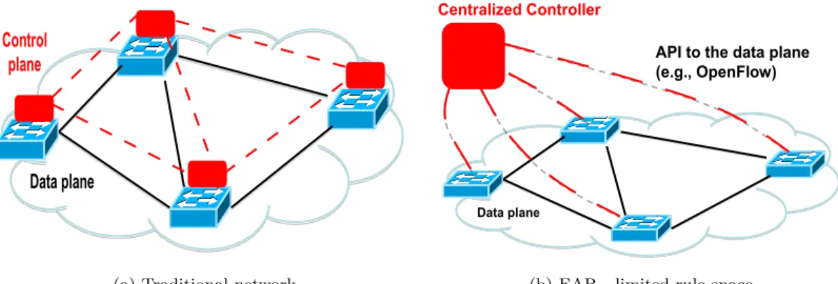
Recent studies have shown that ICT is responsible for 2% to 10% of the worldwide power con-sumption [1, 2]. As estimation, energy requirement for European telecommunication can reach 35.8 TWh in 2020 [3]. Backbone ISP networks currently consume around 10% of the total net-work power requirements and it can increase to 40% by 2017 [4]. Therefore green netnet-working has been attracting a growing attention during the last years (see the surveys [5, 6]). While the traffic load has a marginal influence, the power consumption is mainly due to active elements on IP routers such as ports, line cards, base chassis, etc. [7]. Based on this observation, the energy-aware routing (EAR) approach aims at minimizing the number of used network elements while all the traffic demands are routed without any overloaded links [1, 8]. In fact, turning off entire routers can earn significant energy savings. However, it is very difficult from a practical point of view as it takes time for turning on/off and also reduces life cycle of devices. Therefore, as in prior work [9, 10], we assume to turn off (or put into sleep mode) only links to save energy. Software-defined networking (SDN) in general, and OpenFlow in particular [11], has been attracting a growing attention in the networking research community in recent years. In tradi-tional networks (Fig. 1a), network devices such as routers and switches act as “closed” systems. They work as “black boxes” with applications implemented on them. Users can only control them via limited and vendor-specific control interfaces. Moreover, the data plane (forwarding function) and control plane are integrated in each device, making them quite difficult to deploy new network protocols. SDN is a new networking paradigm that decouples the control plane from the data plane (Fig. 1b). It provides a flexibility to develop and test new network protocols and policies in real networks. OpenFlow has applications in a wide range of networked environments and over past few years, many applications have been built using the OpenFlow API [11]. For instance, the work in [12] describes B4 - one of the first and largest SDN deployments in Google data center network. B4 has been in deployment for three years and real lessons learned show that B4 can efficiently meet application bandwidth demands, supports rapid deployment of new network control services and is robust with failure conditions.
Control plane
Data plane
(a) Traditional network
API to the data plane (e.g., OpenFlow) Centralized Controller
Data plane
(b) EAR - limited rule space
Figure 1: SDN network
In this paper, we focus on one application of the OpenFlow, that is to use OpenFlow to minimize power consumption for an Internet service provider (ISP). As shown in literature, many existing works have used OpenFlow as a traffic engineering approach to deploy EAR in a network. For instance, the authors in [13, 14, 15] have used real testbed with OpenFlow switches to evaluate their energy savings proposals. In these works, the flow table of each switch
is assumed to hold an infinite number of rules. In practice, however, this assumption does not hold, and rule space becomes a significant bottleneck to scaling SDN networks. It is because the flow table is implemented using Ternary Content Addressable Memory (TCAM) which is expensive and power hungry. Therefore, commodity switches typically support just from few hundreds to few thousands of entries [16, 17, 18]. Taking this limitation into account, we show that the rule space constraints are very important in EAR. An inefficient rule allocation can lead to an unexpected routing solution, causing network congestion and affecting QoS.
In summary, we make the following contributions:
• To our best knowledge, this is the first work that defines and formulates the optimizing rule space problem in OpenFlow for EAR using ILP.
• As EAR is known to be NP-hard [?], we propose heuristic algorithm that is effective for large network topologies. By simulations, we show that the heuristic algorithm achieves close-to-optimal solutions obtained by the ILP.
• Using real-life data traffic traces from SNDlib [19], we show energy savings achieved by our approaches. Moreover, we also show other QoS aspects such as link load and routing length of EAR solutions.
The rest of this paper is structured as follows. We summarize related work in Section 2. We present the ILP and heuristic algorithm in Section 3 for the optimizing rule placement problem. Simulation results are shown in Section 4. Finally, we conclude the work in Section 5 and present future work in Section 6.
2
Related Work
2.1
Classical Energy-aware Routing
Starting from the pioneering work of Gupta [8], the idea of power proportionality has gained a growing attention in networking research area [20, 1]. Since power consumption of router is independent from traffic load, people suggested putting network components to sleep in order to save energy. Although power savings is worthwhile, performance effects must be minimal, and fault tolerance must be satisfied. Several proposals have been proposed to find feasible routing solutions while satisfying QoS constraints and being minimal in power consumption. For instance, the authors in [20, 1] use mixed integer programming to optimize router power in a wide area network. Furthermore, other works on saving energy for data centers have also been presented [13, 15]. In general, these works show that up to 50% of network energy can be saved while maintaining the ability to handle traffic surges and guaranteeing QoS.
2.2
Limited Rule Space in OpenFlow Switches
To support a vast range of network applications, OpenFlow rules are more complex than for-warding rules in traditional IP routers. For instance, access-control requires matching on source - destination IP addresses, port numbers and protocol [21] whereas a load balancer may match only on source and destination IP prefixes [22]. These complicated matching can be well sup-ported using TCAM since all rules can be read in parallel to identify the matching entries for each packet. However, as TCAM is expensive and extremely power-hungry, the on-chip TCAM size is typically limited. Many existing works in literature have tried to address this limited rule space problem. For instance, the authors in [23] try to compact the TCAM by using shorter tags
for identifying flows. Another approach is to compress policies on a single switch. For exam-ple, the authors in [24, 25, 26] have proposed algorithms to reduce the number of rules needed to realize policies on a single switch. To the best of our knowledge, the closest papers to our work are from [16, 17]. These works present efficient heuristic rule-placement algorithms that distribute forwarding policies while managing rule-space constraints at each switch. However, they do not rely on the exact meaning of the rules and the rules should not determine the routing of the packet [17]. Therefore, these techniques cannot directly solve the rule-placement problem in EAR. In this work, we focus on EAR where rules explicitly determine the routing of traffic flows. Besides an exact formulation ILP, we also propose efficient heuristic algorithm for large networks.
0
1
2
3
4
5
6
12
12
12
12
5
5
5
4
4
(a) Network and capacity on links
0
1
2
3
4
5
6
(b) EAR - unlimited rule space
0
1
2
3
4
5
6
(c) EAR - limited rule space
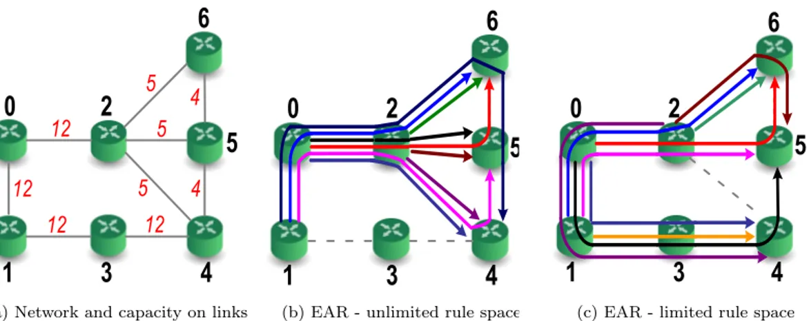
Figure 2: Example of EAR with and without rule space constraints
2.3
Energy Savings with OpenFlow
OpenFlow is a promising method to implement EAR in a network. For instance, the authors in [13] have implemented and analyzed ElasticTree on a prototype testbed built with production OpenFlow switches. The idea is to use OpenFlow to control traffic flows so that it minimizes the number of used network elements to save energy. Similarly, the authors in [15] have set up a small testbed using OpenFlow switches to evaluate energy savings for their model. OpenFlow switches have also been mentioned in many existing works as an example of the traffic engineering method to implement the EAR idea [27, 14]. However, as we can see, the testbed setups with real OpenFlow switches are quite small. For instance, it is with 45 virtual switches onto two 144-port 5406 chassis switches, running OpenFlow v0.8.9 firmware provided by HP Labs [13] or 10 virtual switches on a 48-port Pronto 3240 OpenFlow-enabled switch [15]. However, we argue that when deploying EAR with OpenFlow in real network topologies, much more real OpenFlow switches should be used and they will handle a large amount of flows. In this situation, limited rule space in switches becomes a serious problem since we can not route traffic as expected. Therefore, we present in next Section a novel optimization method to overcome the rule placement problem of OpenFlow in EAR.
3
Optimizing Rule Placement
Routing decision of an OpenFlow switch is based on flow tables implemented in TCAM. Each entry in the flow table defines a matching rule and is associated with an action. Upon receiving a packet, a switch identifies the highest-priority rule with a matching predicate, and performs the corresponding action. A packet that matches no rules is processed using the default rule, which has the lowest-priority. Depending on applications of OpenFlow, the default rule can be dropping packets or forwarding packets to the controller over the OpenFlow channel. In this work, to avoid delay communication between routers and the centralized controller, we consider the default rule which is just to forward packets to a default port (without contacting the controller), and each switch has exactly one default port [28].
Table 1: Traffic demands and routing solutions
Traffic demand Volume Routing solution Routing solution
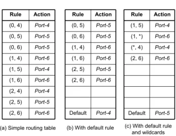
(Fig. 2b) (Fig. 2c) (0, 4) 1 0 - 2 - 4 0 - 1 - 3 - 4 (0, 5) 2 0 - 2 - 5 0 - 1 - 3 - 4 - 5 (0, 6) 2 0 - 2 - 5 - 6 0 - 2 - 5 - 6 (1, 4) 1 1 - 0 - 2 - 6 - 5 - 4 1 - 3 - 4 (1, 5) 3 1 - 0 - 2 - 4 - 5 1 - 0 - 2 - 5 (1, 6) 3 1 - 0 - 2 - 6 1 - 0 - 2 - 6 (2, 4) 1 2 - 4 2 - 0 - 1 - 3 - 4 (2, 5) 1 2 - 5 2 - 6 - 5 (2, 6) 1 2 - 6 2 - 6 Port-6 (1, 4) Port-4 (1, 5) Port-6 (1, 6) Port-4 (2, 4) Port-5 (2, 5) Rule Action (0, 4) Port-4 (0, 5) Port-5 (0, 6) Port-5 (2, 6) Port-6 Port-5 (2, 5) Port-6 (2, 6) Port-6 (1, 6) Port-6 (1, 4) Rule Action (0, 5) Port-5 (0, 6) Port-5 Default Port-4
(a) Simple routing table (b) With default rule (c) With default rule and wildcards Port-6 (1, *) Port-4 (*, 4) Port-4 (1, 5) Rule Action (2, 6) Port-6 Default Port-5
Figure 3: Routing table at router 2 for routing of Fig. 2b
As presented in Section 2.2, the routing table in OpenFlow switch has limited size. This limitation is very important in EAR as we show in Fig. 2. Assume that there are 9 traffic demands with volumes as shown in Table 1. The network topology and capacity on links are shown in Fig. 2a. For ease of reading, Table 1 also shows the routing of each traffic flow in Fig. 2b and Fig. 2c. These routing solutions are found by using the ILP in Section 3.1. As the classical EAR approach, Fig. 2b shows an optimal solution since it satisfies capacity constraints
and uses a minimum number of active links (7 links). It is noted that, as the objective of EAR is to minimize the number of used links and because of the capacity constraints, some traffic flows may be routed via long paths. For instance, the flow (1, 4) is routed via five hops while its shortest path is only two hops. One possible way to avoid this is to have some constraints that limit the stretch of the path of each flow.
Assume now that the routing table of router contains rules which are the mapping of [(src, dest) : port-to-foward]. As the routing in Fig. 2b, the router 2 needs to forward 9 flows, hence a simple routing table can be as Fig. 3a. However, we can reduce the size of the routing table by using a default rule (Fig. 3b), or combining default rule and wildcards (Fig. 3c). Note that the rules [(0, 5): port-5] and [(0, 6): port-5] of Fig. 3b can not be combined as [(0, *): port-5]. It is because the flow (0, 4) will go to port-5 when it should go to port-4. In Fig. 3c, as the rule (1, 5) has higher priority than the rule (1, *), the flow (1, 5) is forwarded to port-4 while the flows (1, 4) and (1, 6) are forwarded to port-6 with the rule (1, *).
Assume that we implement EAR on SDN network where each router can install at most 4 rules. As a result, the router 2 can install only 3 distinct rules and 1 default rule. However, as we have shown, the minimum routing table contains 5 rules (Fig. 3c). Therefore, in this situation, some flows need to be routed using the default port. For instance, if the flow (2, 6) in Fig. 3c goes to the default port-5, then the link (2, 5) will be overloaded. It is also easy to check that, with the rule capacity equals to 4 and a set of active links as in Fig. 2b, it is not possible to find a routing solution that satisfies both capacity constraints on links and rule space constraints on routers. However, if we consider the rule space constraints as inputs of the problem, we can find a feasible solution as Fig. 2c. Actually, since we add more constraints, the EAR with rule space is able to save less energy with respect to the classical EAR. For instance, there is only 1 inactive link in Fig. 2c while we can turn off 2 links and save more energy in Fig. 2b.
As we have shown in the example, the limited rule space is very important in EAR. Inefficient rule placement can cause unexpected routing solution, and hence result in network congestion. To overcome this problem, we present in this section a precise formulation (Integer Linear Pro-gram) and heuristic approach of the optimizing rule placement for energy-aware routing problem. However, we note that the current algorithms can find optimal solution of energy consumption (or close-to-optimal if it is heuristic) in case we consider the default rule but not the wildcard. If the rule space is very limited and we can not find feasible solution, we can apply the work in “compressing policy on a single switch” [24, 25, 26] as a post-processing step to reduce more the routing table size. This post-processing step will be integrated into our algorithms in the future work.
3.1
Integer Linear Program
We consider a backbone network as an undirected graph G = (V, E). The nodes in V describe routers and the edges in E present connections between those routers. We denote by Dst the demand of traffic flow from node s to node t such that Dst≥ 0, s, t ∈ V, s ̸= t. We assume that the capacity of links and the rule space at routers are constants. The task is to find a feasible routing for all traffic flows, respecting the capacity and the rule space constraints and being minimal in energy consumption.
We first define the following notations and then formulate the problem as Integer Linear Program:
• D: a set of all traffic demands to be routed. • Dst∈ D: demand of the traffic flow from s to t. • Cuv: capacity of a link (u, v).
• µ ∈ (0, 1]: maximum link utilization that can be tolerated. It is normally set to a small value, e.g. µ = 0.5.
• Cu: maximum number of rules can be installed at router u. • N (u): the set of neighbors of u in the graph G.
• xuv: binary variable to indicate if the link (u, v) is active or not. • fst
uv: a flow (s, t) that is routed on the link (u, v) by a distinct rule. We call fuvst as normal flow.
• gst
uv: a flow (s, t) that is routed on the link (u, v) by a default rule. guvst is called default flow to distinguish from the normal flow fst
uv .
• kuv: binary variable to indicate if the default port of the router u is to go to v or not.
min ∑ (u,v)∈E xuv (1) s.t. ∑ v∈N(u) (fst vu+ g st vu− g st uv− f st uv) = −1 if u = s, 1 if u = t, 0 else ∀u ∈ V, (s, t) ∈ D (2) fuvst + f st vu+ g st uv+ g st vu ≤ 1 ∀(u, v) ∈ E, (s, t) ∈ D (3) ∑ (s,t)∈D Dst(fst uv+ f st vu+ g st uv+ g st vu) ≤ µCuvxuv ∀(u, v) ∈ E (4) ∑ (s,t)∈D ∑ v∈N(u) fst uv ≤ Cu− 1 ∀u ∈ V (5) gst uv ≤ kuv ∀(u, v) ∈ E, (s, t) ∈ D (6) ∑ v∈N(u) kuv ≤ 1 ∀u ∈ V (7) xuv, fuvst, g st uv, kuv∈ {0, 1} ∀(u, v) ∈ E, (s, t) ∈ D (8) The objective function (1) minimizes the power consumption of the network represented by the number of active links. Constraints (2) are the flow conservation constraints. It makes sure that the total flows entering and leaving a router are the same (except the source and the destination nodes). It is noted that a normal flow entering a router can become a default flow on outgoing link and vice versa. Constraints (3) are used to ensure that a flow (s, t) on a
link (u, v) cannot be both normal (fst
uv) and default flow (gstuv) at the same time. We consider an undirected link capacity model [29] in which the capacity of a link is shared between the traffic in both directions. Constraints (4) limit the available capacity of a link. Constraints (5) denote rule capacity constraints where we reserve one rule at each router to be the default rule. Constraints (6) and (7) are used to fix only one default port for each router.
3.2
Heuristic Algorithm
Since energy-aware routing problem is known to be NP-Hard [?], it is very challenging to find an exact solution. Therefore, we present in this section an efficient greedy heuristic for large networks. In summary, the heuristic algorithm works through two steps:
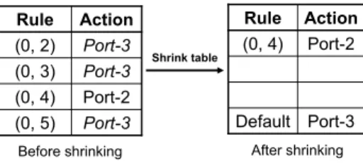
- Step 1: starting from the whole network, we compute feasible routing with respect capacity and rule space constraints as described in Algorithm 1, Algorithm 2 and Algorithm 3. For each router u ∈ V , we keep the two sets FuandGu containing normal and default flows, respectively. In the beginning, we are freely to assign distinct rules for flows. When the routing table is full (|Fu| = Cu), we try to shrink it as Fig. 4. The idea of shrinking table is to choose a port that carries most of traffic flows to become the default port. As a result, the number of installed rules is reduced and we have available space to install new rules.
- Step 2: trying to remove in priority links that are less loaded (Algorithm 4 ). The idea behind this algorithm is that we try to turn off the low loaded links and to accommodate their traffic on other links to reduce the total number of active links.
Port-3 (0, 5) Port-2 (0, 4) Port-3 (0, 3) Port-3 (0, 2) Action Rule Port-3 Default Port-2 (0, 4) Action Rule Shrink table
Before shrinking After shrinking Figure 4: Routing table at a router
B A C D 5/10 5/10 5/10 10/30 10 B A C D
Node A has installed 5 rules while CA= 10. Cmax= 30 wAC= 30*10/30 = 10 wCA= 30*5/10 = 15 15 15 15 15 15 15 10
Undirected graph G Directed graph G’
weight
Figure 5: Example of updating link weight
An example of computing link weights (Algorithm 2 ) is shown in Fig. 5. The idea is that we would like to perform a rule-balancing between routers on network. Assume that the next demand is (A, D), then the routing solution using shortest path is (A, C, D). It is better than (A, B, D) since node C still has much more available rule space. Note that, we use the digraph G′ only for finding shortest path, other operations (remove links, update residual capacity) are done on the undirected graph G.
Algorithm 1:Finding a feasible routing
Input: An undirected graph G = (V, E), link capacity Ce ∀e ∈ E, rule space capacity Cu∀u ∈ V and a set of demands D.
Ouput: routing solution on graph G. Residual capacity Re= Ce ∀e ∈ E; Initially,Fu= ∅ and Gu= ∅ ∀u ∈ V ;
Creating directed graph G′= (V, E′) from G where ∀(u, v) ∈ E, we add both directions (u, v) and (v, u) to E′ (Fig. 5). Initial weight on link we= 1 ∀e ∈ E′;
whileDst∈ D has no assigned route do
find the shortest path Pst on G′ such that Re≥ Dst ∀e ∈ Pst; assign the routing Pst to the demand Dst;
update Re:= Re− Dst ∀e ∈ Pst;
update link weights proportionally to the size|Fu| as Algorithm 2; if|Fu| == Cu, shrink table at u ∀u ∈ Pst;
updateFu andGu ∀u ∈ Pst using Algorithm 3; end
return the routing (if it exists) assigned forD
Algorithm 2:Updating link weight
Input: An undirected graph G = (V, E), a set of normal flows Fu ∀u ∈ V and a maximum value of rule space capacity Cmax= max(Cu) ∀u ∈ V .
Ouput: weight setting on links of G′. Create a digraph G′ = (V, E′) as Fig. 5. for(u, v) in E′ do
compute rule utilization at v: Uv= Cmax× |Fv|/Cv; update wuv= max(Uv, 1);
end
Algorithm 3:Updating Fu andGu
Input: An undirected graph G = (V, E), the shortest path Pst found in Algorithm 1, the setFu andGu ∀u ∈ Pst and the default port of each router d(u) ∀u ∈ Pst.
Ouput: Updated sets ofFuandGu ∀u ∈ V . foru ∈ Pst do
forv ∈ G.neighbor(u) do
if (u, v) ∈ Pst andv == d(u) then Gu= Gu∪ gst
uv
else if (u, v) ∈ Pst andv ̸= d(u) then Fu= Fu∪ fst
uv end
end end
Algorithm 4: Removing less loaded links
Input: An undirected graph G = (V, E), link capacity Ceand residual capacity Re∀e ∈ E. Ouput: routing solution on a set of active links.
whileedges can be removed do
remove the edge e that has not been chosen and has smallest value Ce/Re; compute a feasible routing with the Algorithm 1;
if no feasible routing exists, put e back to G; end
return the feasible routing if it exists.
4
Simulation Results
We solved the ILP model with IBM CPLEX 12.4 [30]. All computations were carried out on a computer equipped with 2.7 Ghz Intel Core i7 and 8 GB RAM. We consider real-life traffic traces collected from SNDlib [19]. To compare between optimal and heuristic solutions, we use a small network as Atlanta network (V = 15, E = 22, |D| = 210). As mentioned in [16, 17], the routing table can support from 750 to few thousands of rules. Thus the problem of limited rule space can be serious only for large networks where thousands of concurrent flows need to be routed. To show that this is a realistic problem, we use three of the largest network topologies in SNDlib: the ta2 (Telekom Austria: V = 65, E = 108, |D| = 4160), zib54 (Zuse-Institut Berlin: V = 54, E = 81, |D| = 2862) and germany50 (V = 50, E = 88, |D| = 2450). Note that, in SNDlib, low traffic pairs are not reported. So if a traffic pair does not appear in SNDlib, we add this demand to the model with a small value.
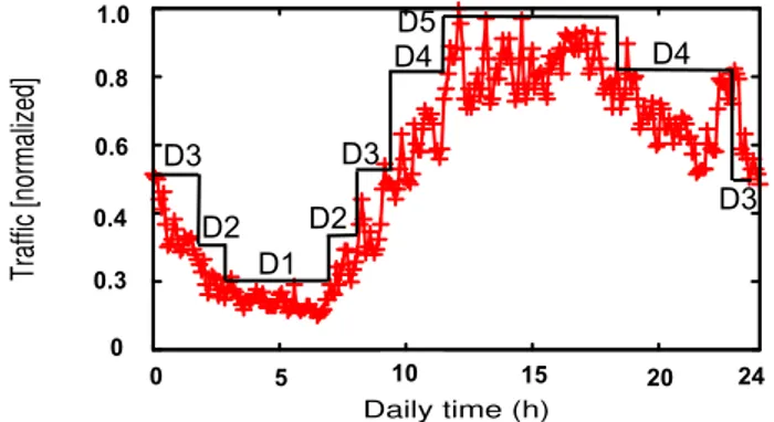
0 0.2 0.4 0.6 0.8 1 0 5 10 15 20 Traffic [normalized] Daily time (h) D1 D2 D3 D2 D4 D4 D5 D3 D3 0.3 0.4 0 0.6 0.8 1.0 0 5 10 15 20 24
Figure 6: Daily traffic in multi-period
In our test instances, five traffic matrices (D1 - D5) are used to represent daily traffic pattern (Fig. 6). Since traffic load is low, we use the traffic matrix found in SNDlib as D1. To achieve a network with high link utilization, we scale D1 with a factor of 1.5, 2.0, 2.5 and 3.0, and they form D2 - D5, respectively. Then, we apply the ILP or heuristic algorithm to find routing solution for each traffic matrix.
4.1
Optimal vs. Heuristic Solutions
Assume that each router on the network has the same rule capacity represented by Cu= (p×|D|) where p ∈ (0, 1] and |D| is the total demands. To compare between the optimal and the heuristic
solutions, we use a small network as Atlanta network and the traffic matrix D1. The value of Cu is varied as we change the parameter p. Energy savings is computed as the number of link to sleep divided by the total number of links on the network (|E|).
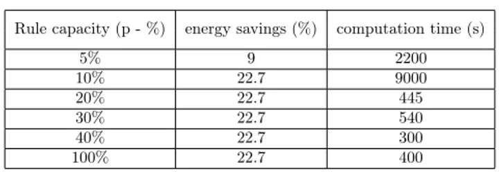
Table 2: Atlanta network (optimal solution)
Rule capacity (p - %) energy savings (%) computation time (s)
5% 9 2200 10% 22.7 9000 20% 22.7 445 30% 22.7 540 40% 22.7 300 100% 22.7 400
Table 3: Atlanta network (heuristic solution)
Rule capacity (p - %) energy savings (%) computation time (s)
16% 4.5 < 10
20% 13.6 < 10
30% 18.2 < 10
40% 18.2 < 10
100% 18.2 < 10
As shown in Table 1 and Table 2, the ILP model can find solution for very limited rule space (p = 5%) meanwhile it is 16% for the heuristic algorithm. Similarly, for energy savings, a quite big gap happens when p is small (e.g. p ≤ 16%). However, when the rule space capacity is large enough, e.g. p = 30%, the gaps between the optimal and the heuristic solutions are quite small. Moreover, the heuristic algorithm gains a lot in computation time. For instance, the ILP model can take up to 9000 (s) to find solution meanwhile it is always less than 10 (s) for the heuristic algorithm.
4.2
Heuristic Solutions for Large Networks
4.2.1 Rule allocation at routers
We assume that all the routers have the same rule space capacity Cu= 750 [17]. As the classical EAR approach, we use the heuristic algorithm in [?] as the case that there is no limit in rule space at routers. We run this algorithm on germany50, zib54 and ta2 networks to see if the rule space constraints are violated or not.
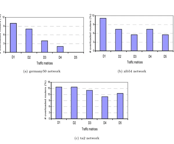
As shown in Fig. 7a, Fig. 7b and Fig. 7c, most of the cases (except D5 of germany50 network), there are always routers that use more than 750 rules in their routing tables. In zib54 network (resp. ta2 network), from 6% to 11% (resp. 11% to 16%) of routers exceed their rule space capacities. In germany50 network, with the D5 traffic matrix, there is no router that uses more than 750 rules. For other traffic matrices, from 2% to 10% of the routers are overloaded in rule space (Fig. 7a). Therefore, the limited rule space is really a problem in real networks. This problem is extremely important in energy-aware routing since we cannot route traffic as expected. The number of routers overloaded in rule space depends on the traffic matrix. An accurate prognosis is difficult since the algorithm in [?] does not care at all about the rule space
0 3 6 9 12 1 2 3 4 5 Traffic matrices D1 Traffic matrices # o ve r lo a d e d r o u te r s ( % ) D2 D3 D4 D5
(a) germany50 network
0 3 6 9 12 1 2 3 4 5 Traffic matrices D1 Traffic matrices # o ve r lo a d e d r o u te r s ( % ) D2 D3 D4 D5 (b) zib54 network 0 3 6 9 12 15 18 1 2 3 4 5 traffic matrices D1 Traffic matrices # o ve r lo a d e d r o u te r s ( % ) D2 D3 D4 D5 (c) ta2 network
Figure 7: Number of overloaded routers in germany50, zib54 and ta2 networks
capacity. However, in general, the larger the network we consider, the more routers that are overload in rule space.
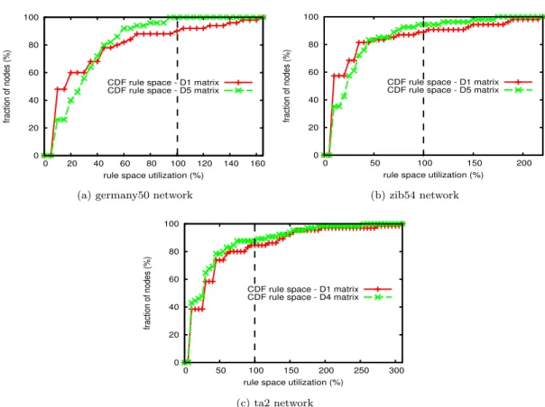
To take a closer look at rule space allocation, we draw cumulative distribution function (CDF) for rule utilization at each router (Fig. 8a, Fig. 8b and Fig. 8c). When a rule space utilization is larger than 100%, it means that the router has used more than 750 rules. Based on Fig. 7a, Fig. 7b and Fig. 7c, we can find the traffic matrices that cause the maximum and the minimum number of routers violating their rule space constraints. We call these traffic matrices as the max-over-rule and the min-over-rule, respectively. For instance, in case of germany50 network, D1 is the max-over-rule and D5 is the min-over-rule. For each network, we draw two CDFs of rule utilization for the max-over-rule and the min-over-rule cases. As shown in Fig. 8a, Fig. 8b and Fig. 8c, the CDF of rule space allocation of the two cases are quite similar. However we can see in the max-over-rule case, more fractions of routers are overloaded. For instance, in Fig. 8b, only 89% of routers are less than 100% rule space utilization in the max-over-rule case (D1), meanwhile it is 94% of routers in the min-over-rule case (D5). In general, the larger the network is, the more rule space is needed at routers. For example, the maximum rule utilization for germany50, zib54 and ta2 networks are 165%, 220% and 310%, respectively.
0 20 40 60 80 100 0 20 40 60 80 100 120 140 160 fraction of nodes (%)
rule space utilization (%) CDF rule space - D1 matrix CDF rule space - D5 matrix
(a) germany50 network
0 20 40 60 80 100 0 50 100 150 200 fraction of nodes (%)
rule space utilization (%) CDF rule space - D1 matrix CDF rule space - D5 matrix
(b) zib54 network 0 20 40 60 80 100 0 50 100 150 200 250 300 fraction of nodes (%)
rule space utilization (%) CDF rule space - D1 matrix CDF rule space - D4 matrix
(c) ta2 network
Figure 8: CDF rule space utilization in germany50, zib54 and ta2 networks
4.2.2 Energy savings
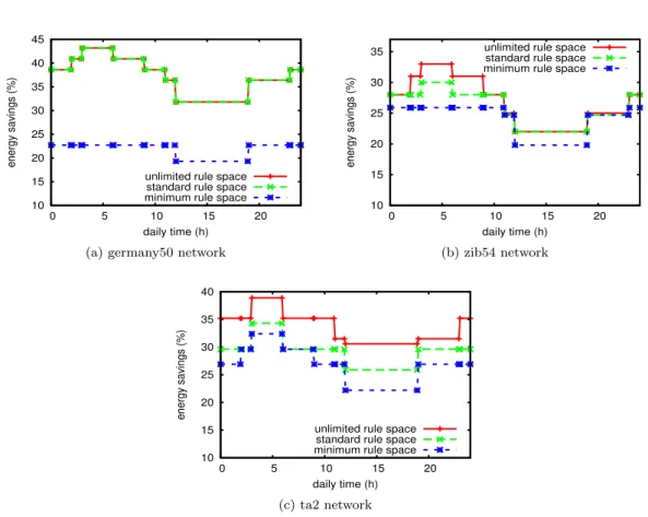
We collect energy savings for each network in three cases: the minimum, the standard and the unlimited rule spaces. In the standard case, each router can install at most 750 rules (Cu= 750). To find the minimum rule space, we reduce the value of Cuuntil we get a minimum value of Cu for which it is possible to find a feasible solution. The minimum values of Cu for germany50, zib54 and ta2 networks are 227, 670 and 695, respectively. The unlimited rule space case is equivalent to the classical EAR model in which we do not consider at all rule space constraints at routers. In general, as shown in Fig. 9a, Fig. 9b and Fig. 9c, the larger the rule space at routers is, the more flexible routing solutions we have and more energy can be saved for the network. The energy savings gap between the standard and the unlimited rule space cases is quite small. In some traffic matrices, both cases offer the same amount of energy savings. For instance in germany50 network, the standard and unlimited cases offer the same amount of energy savings. It shows that using a smart rule allocation, it is possible to achieve energy savings as high as the classical EAR while respecting the rule space constraints. The maximum energy savings gaps of the standard and the unlimited cases are 3% and 5.6% for zib54 and ta2 networks, respectively. As expected, energy is saved less in the minimum rule space case. It is because we do not have enough installed rules to route traffic in a better way. As shown in Fig. 9a, the energy savings gap between the minimum and standard cases is quite big. This can be explained as the difference between the minimum and standard values of Cuin germany50 network is quite large.
10 15 20 25 30 35 40 45 0 5 10 15 20 energy savings (%) daily time (h) unlimited rule space
standard rule space minimum rule space
(a) germany50 network
10 15 20 25 30 35 0 5 10 15 20 energy savings (%) daily time (h) unlimited rule space standard rule space minimum rule space
(b) zib54 network 10 15 20 25 30 35 40 0 5 10 15 20 energy savings (%) daily time (h) unlimited rule space standard rule space minimum rule space
(c) ta2 network
Figure 9: Energy savings in daily time in germany50, zib54 and ta2 networks
4.2.3 Route length
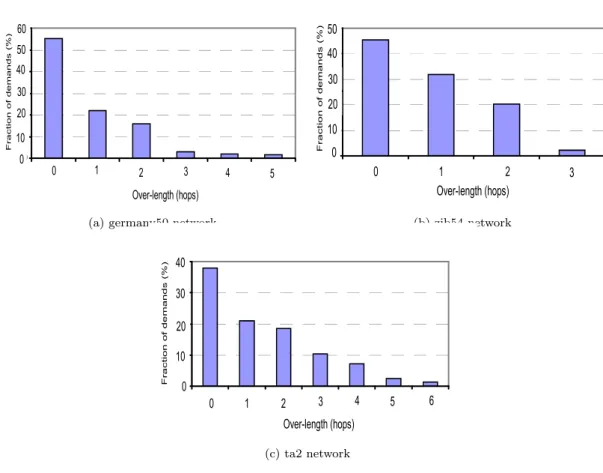
Intuitively, EAR would affect the length of routing flows as we redirect traffic flows to minimize the number of active links. In Fig. 10a, Fig. 10b and Fig. 10c, we evaluate the impact of EAR on routing length with respect to the shortest path routing. For each traffic demand, we collect the length of its routing flow and the corresponding shortest path. We use the notation over-length to denote the difference (in number of hops) between the length of the routing solution and the shortest path. When over-length is equal to 0, it means that the routing solution is exactly the shortest path. As shown in Fig. 10a, Fig. 10b and Fig. 10c, a large fraction of the demands follow their shortest paths. Indeed, in the heuristic algorithm, we use the shortest path to find routing solution. In germany50 and zib54, the maximum number of additional hops for a demand is 3 and 5 hops, respectively. The ta2 network is larger, up to 6 hops can be added to a demand, but it happens only for 1.4% of the demands. However, if latency is important, especially for sensitive delay applications such as voice or video streaming, we can add constraints to limit the route length so that it will not excess a predefined threshold value.
4.2.4 Link load
In this simulation, for simplicity, we set the maximum link utilization µ = 100%. Intuitively, EAR would affect the utilization of links as fewer links are used to carry traffic. In this subsection, we evaluate the impact of EAR on link utilization. We draw the CDFs of link load of germany50,
0 10 20 30 40 50 60 1 12 3 4 5 6 0 2 3 0 10 30 20 40 Over-length (hops) F r a ct io n o f d e m a n d s ( % ) 4 5 50 60
(a) germany50 network
0 10 20 30 40 50 1 12 3 4 0 2 3 0 10 30 20 40 50 Over-length (hops) F r a ct io n o f d e m a n d s ( % ) (b) zib54 network 0 10 20 30 40 10 12 23 34 5 6 7 0 10 30 20 40 Over-length (hops) F r a ct io n o f d e m a n d s ( % ) 4 5 6 (c) ta2 network
Figure 10: Over-length of demands in germany50, zib54 and ta2 networks
zib54 and ta2 networks in Fig. 11a, Fig. 11b and Fig. 11c. For each network, we collect traffic load of the lowest (D1) and the highest (D5) traffic matrices. As shown in Fig. 11a, Fig. 11b and Fig. 11c, the solutions with D5 have heavier link load than in D1. It means for low traffic matrix, fewer links are used but the link load does not increase too much. High link utilization (e.g. with D5 traffic matrix) can affect QoS as it causes packet drop and long queuing delay. One possible way to overcome this problem is to set the maximum link utilization to a small value, e.g. µ = 50%.
5
Conclusions
To the best of our knowledge, this is the first work considering rule space constraints of OpenFlow switch in energy-aware routing. We argue that, in addition to capacity constraint, the rule space is also important as it can change the routing solution and affects QoS. Based on simulations with real traffic traces, we show that our smart rule allocation can achieve high energy efficiency for a backbone network while respecting both the capacity and the rule space constraints.
0 20 40 60 80 100 0 20 40 60 80 100 fraction of links (%) link utilization (%) traffic load with D1 traffic load with D5
(a) germany50 network
0 20 40 60 80 100 0 20 40 60 80 100 fraction of links (%) link utilization (%) traffic load with D1 traffic load with D5
(b) zib54 network 0 20 40 60 80 100 0 20 40 60 80 100 fraction of links (%) link utilization (%) traffic load with D1 traffic load with D5
(c) ta2 network
Figure 11: CDF of link load in germany50, zib54 and ta2 networks
6
Future work
In this paper, to deal with the traffic variation, daily time periods are characterized by different traffic levels and in each period, a single traffic matrix is assumed to be accurately collected. As traffic matrices are considered independently, different sets of rules are installed on routers for each traffic matrix. However, from the view point of traffic engineering, frequent changes in the routing configuration can cause network disruption [9, 31]. Therefore, we argue that the future work should take into account the stability of rule setting for the energy-aware traffic engineering problem. Rather than computing a new rule placement from scratch for each traffic matrix, we must allow to incrementally update the rule setting to minimize the computation time and avoid service deteriorations for end users.
Although the power savings is worthwhile, the performance effects must be minimal. The further work should consider the trade-offs between energy efficiency, performance and robust-ness. For instance, one approach is to perform load-balancing on top of the EAR techniques [32]. This helps to achieve energy efficient network but without sacrificing the traditional traffic en-gineering. In addition, other performance effects such as network fault-tolerance, packet latency should be also considered.
As prior works in literature, OpenFlow has been used to evaluate energy savings in data center network [13, 15]. However, as the limited rule space is ignored, the evaluation may not be as expected, especially in large scale data center networks. We propose as a future work to
re-evaluate these models while taking into account rule space constraints. This will provide a more accurate evaluation of energy efficiency for the network.
References
[1] L. Chiaraviglio, M. Mellia, F. Neri, “Minimizing ISP Network Energy Cost: Formulation and Solutions”, IEEE/ACM Transaction in Networking 20 (2011) 463 – 476.
[2] Global action plan, http://globalactionplan.org.uk (2007).
[3] R. Bolla, F. Davoli, R. Bruschi, K. Christensen, F. Cucchietti, S. Singh, “The Potential Impact of Green Technologies in Next-generation Wireline Networks: Is There Room for Energy Saving Optimization?”, IEEE Communications Magazine 49 (2011) 80 – 86. [4] C. Lange, “Energy-related aspects in backbone networks”, in: 35th European Conference on
Optical Communication, 2009.
[5] A. P. Bianzino, C. Chaudet, D. Rossi, J. Rougier, “A Survey of Green Networking Research”, IEEE Communication Surveys and Tutorials 14 (2012) 3 – 20.
[6] R. Bolla, R. Bruschi, F. Davoli, F. Cucchietti, “Energy Efficiency in the Future Internet: A Survey of Existing Approaches and Trends in Energy-Aware Fixed Network Infrastructures”, IEEE Communication Surveys and Tutorials 13 (2011) 223 – 244.
[7] P. Mahadevan, P. Sharma, S. Banerjee, “A Power Benchmarking Framework for Network Devices”, in: International Conferences on Networking (IFIP NETWORKING), 2009, pp. 795–808.
[8] M. Gupta, S. Singh, “Greening of the Internet”, in: ACM Special Interest Group on Data Communication (SIGCOMM), 2003, pp. 19–26.
[9] L. Chiaraviglio, A. Cianfrani, E. L. Rouzic, M. Polverini, “Sleep Modes Effectiveness in Backbone Networks with Limited Configurations”, Computer Networks 57 (2013) 2931– 2948.
[10] F. Giroire, J. Moulierac, T. K. Phan, F. Roudaut, “Minimization of Network Power Con-sumption with Redundancy Elimination”, in: International Conferences on Networking (IFIP NETWORKING), 2012, pp. 247–258.
[11] N. McKeown, T. Anderson, H. Balakrishnan, G. Parulkar, L. Peterson, J. Rexford, S. Shenker, J. Turner, “Openflow: Enabling Innovation in Campus Networks”, ACM Com-puter Communication Review 38 (2008) 69 – 74.
[12] S. Jain, A. Kumar, S. Mandal, J. Ong, L. Poutievski, A. Singh, S. Venkata, J. Wanderer, J. Zhou, M. Zhu, J. Zolla, U. Holzle, S. Stuart, A. Vahdat, “B4: Experience with a Globally-Deployed Software Defined WAN”, in: ACM Special Interest Group on Data Communication (SIGCOMM), 2013.
[13] B. Heller, S. Seetharaman, P. Mahadevan, Y. Yiakoumis, P. Sharma, S. Banerjee, N. McK-eown, “ElasticTree: Saving Energy in Data Center Networks”, in: USENIX conference on Networked systems design and implementation (NSDI), 2010.
[14] N. Vasic, D. Novakovic, S. Shekhar, P. Bhurat, M. Canini, D. Kostic, “Identifying and Using Energy-Critical Paths”, in: ACM Conference on Emerging Networking Experiments and Technologies (CoNEXT), 2011.
[15] X. Wang, Y. Yao, X. Wang, K. Lu, Q. Cao, “CARPO: Correlation-Aware Power Optimiza-tion in Data Center Networks”, in: Annual Joint Conference of the IEEE Computer and Communications Societies (INFOCOM), 2012.
[16] N. Kang, Z. Liu, J. Rexford, D. Walker, “Optimizing the “One Big Switch” Abstraction in Software-Defined Networks”, in: ACM Conference on Emerging Networking Experiments and Technologies (CoNEXT), 2013.
[17] Y. Kanizo, D. Hay, I. Keslassy, “Palette: Distributing Tables in Software-defined Networks”, in: IEEE INFOCOM Mini-conference, 2013.
[18] B. Stephens, A. Cox, W. Felter, C. Dixon, J. Carter, “PAST: Scalable Ethernet for Data Centers”, in: ACM Conference on Emerging Networking Experiments and Technologies (CoNEXT), 2012.
[19] S. Orlowski, R. Wessäly, M. Pióro, A. Tomaszewski,
SNDlib 1.0 - survivable network design library, Networks 55 (3) (2010) 276–286. URL http://sndlib.zib.de
[20] J. Chabarek, J. Sommers, P. Barford, C. Estan, D. Tsiang, S. Wright, “Power Awareness in Network Design and Routing”, in: IEEE International Conference on Computer Communi-cations (INFOCOM), 2008.
[21] M. Casado, M. J. Freedman, J. Pettit, J. Luo, N. Gude, N. McKeown, S. Shenker, “Rethink-ing Enterprise Network Control”, IEEE/ACM Transaction in Network“Rethink-ing 17 (2009) 1270 – 1283.
[22] R. Wang, D. Butnariu, J. Rexford, “OpenFlow-based Server Load Balancing Gone Wild”, in: USENIX Conference on Hot Topics in Management of Internet, Cloud, and Enterprise Networks and Services (Hot-ICE), 2011.
[23] K. Kannan, S. Banerjee, “Compact TCAM: Flow Entry Compaction in TCAM for Power Aware SDN”, in: Distributed Computing and Networking (ICDCN), 2013, pp. 439–444. [24] D. L. Applegate, G. Calinescu, D. S. Johnson, H. Karloff, K. Ligett, J. Wang, “Compressing
Rectilinear Pictures and Minimizing Access Control Lists”, in: ACM-SIAM Symposium on Discrete Algorithms (SODA), 2007.
[25] C. R. Meiners, A. X. Liu, E. Torng, “TCAM Razor: A Systematic Approach Towards Min-imizing Packet Classifiers in TCAMs”, in: IEEE/ACM Transaction in Networking, Vol. 18, 2010, pp. 490 – 500.
[26] C. R. Meiners, A. X. Liu, E. Torng, “Bit Weaving: A Non-prefix Approach to Compressing Packet Classifiers in TCAMs”, IEEE/ACM Transaction in Networking 20 (2012) 488 – 500. [27] A. R. Curtis, J. C. Mogul, J. Tourrilhes, P. Yalagandula, “DevoFlow: Scaling Flow Man-agement for High-Performance Networks”, in: ACM Special Interest Group on Data Com-munication (SIGCOMM), Vol. 41, 2011, pp. 254 – 265.
[28] B. A. A. Nunes, M. Mendonca, X. N. Nguyen, K. Obraczka, T. Turletti, “A Survey of Software-Defined Networking: Past, Present, and Future of Programmable Networks”, IEEE Communications Surveys and Tutorials (2013) 1 – 18.
[29] C. Raack, A. M. C. A. Koster, S. Orlowski, R. Wessäly, “On Cut-based Inequalities for Capacitated Network Design Polyhedra”, Networks 57 (2011) 141 – 156.
[30] IBM ILOG, CPLEX Optimization Studio 12.4.
[31] B. Fortz, M. Thorup, “Optimizing OSPF/IS-IS Weights in a Changing World”, IEEE Journal on Selected Areas in Communications 20 (2002) 756–767.
[32] F. Francois, N. Wang, K. Moessner, S. Georgoulas, “Green IGP Link Weights for Energy-efficiency and Load-balancing in IP Backbone Networks”, in: International Conferences on Networking (IFIP NETWORKING), 2013, pp. 1–9.
2004 route des Lucioles - BP 93 06902 Sophia Antipolis Cedex
BP 105 - 78153 Le Chesnay Cedex inria.fr