HAL Id: hal-00986388
https://hal.archives-ouvertes.fr/hal-00986388
Submitted on 6 May 2014
HAL is a multi-disciplinary open access
archive for the deposit and dissemination of
sci-entific research documents, whether they are
pub-lished or not. The documents may come from
teaching and research institutions in France or
abroad, or from public or private research centers.
L’archive ouverte pluridisciplinaire HAL, est
destinée au dépôt et à la diffusion de documents
scientifiques de niveau recherche, publiés ou non,
émanant des établissements d’enseignement et de
recherche français ou étrangers, des laboratoires
publics ou privés.
Background fluorescence reduction and absorption
correction for fluorescence reflectance imaging
Frederic Fantoni, Lionel Herve, V. Poher, S. Gioux, Jerome Mars, Jean-Marc
Dinten
To cite this version:
Frederic Fantoni, Lionel Herve, V. Poher, S. Gioux, Jerome Mars, et al.. Background fluorescence
reduction and absorption correction for fluorescence reflectance imaging. BIOS2014, SPIE Photonics
West, Feb 2014, San Francisco, United States. pp.8935-34, �10.1117/12.2037600�. �hal-00986388�
Background fluorescence reduction and absorption correction
for fluorescence reflectance imaging
Fantoni F.
a, Herv´e L.
a, Poher V.
a, Gioux S.
b, Mars J. I.
c, and Dinten J.M.
a aCEA, Leti, MINATEC Campus, 17 rue des Martyrs, F38054 GRENOBLE, Cedex 9, France;
b
Beth Israel Deaconess Medical Center, Medicine/SL 436D 330 Brookline Ave Boston, MA
02215, USA;
c
GIPSA Lab, UMR 5216 CNRS - Grenoble INP - Universit´e Joseph Fourier - Universit´e
Stendhal, 11 rue des Math´ematiques, F - 38402 SAINT MARTIN D’HERES Cedex, France
ABSTRACT
Intraoperative fluorescence imaging in reflectance geometry (FRI) is an attractive imaging modality as it allows to noninvasively monitor the fluorescence targeted tumors located below the tissue surface. Some drawbacks of this technique are the background fluorescence decreasing the contrast and absorption heterogeneities leading to misinterpretations concerning fluorescence concentrations.
We presented a FRI technique relying on a laser line scanning instead of a uniform illumination. Here, we propose a correction technique based on this illumination scheme. We scan the medium with the laser line and acquire at each position of the line both fluorescence and excitation images. We then use the finding that there is a relationship between the excitation intensity profile and the background fluorescence one. This allows us to predict the amount of signal to subtract to the fluorescence images to get a better contrast. As the light absorption information is contained both in fluorescence and excitation images, this method also permits us to correct the effects of absorption heterogeneities, leading to a better accuracy for the detection.
This technique has been validated on simulations (with a Monte-Carlo code and with the diffusion approxi-mation using NIRFAST) and experimentally with tissue-like liquid phantoms with different levels of background fluorescence. Fluorescent inclusions are observed in several configurations at depths ranging from 1 mm to 1 cm. Results obtained with this technique are compared to those obtained with a more classical wide-field detection scheme for the contrast enhancement and to the fluorescence to excitation ratio approach for the absorption correction.
Keywords: diffuse optics, near infrared, molecular imaging, laser line illumination
1. INTRODUCTION
The attention to molecular imaging has increased for the past few years,1–4 due to the recent availability of fluorochromes which allow the study of gene expression, protein function and interactions, and a large number of cellular processes in a minimally invasive way.
Molecular imaging presents several advantages: it offers good sensitivity when the observed objects are close to the surface, is generally fast (acquisition times typically range from a fraction of seconds to minutes), the implementations are easy, low cost and compact.
On the other hand, this technique suffers from important limitations. One of them is due to the background noise caused by excitation leaks and fluorescence from superficial layers. While the natural fluorescence of tissues may be used as a means of study,5–8 it is an obstacle for fluorescence reflectance imaging because it reduces the addressed depth several millimeters since the detected signals decrease exponentially with depth while the background noise remains the same.
Fluorescence reflectance imaging is usually performed with a wide-field detection scheme (referred as WF-FRI), contrary to our line scanning approach which gives us access to more information. We scan the medium with the laser line and acquire at each position of the line both fluorescence and excitation images. By using the
relationship between the excitation intensity profile and the background fluorescence one, we are able to predict the amount of signal to subtract to the fluorescence images to get a better contrast. We will also show how this method permits us to correct the effects of absorption heterogeneities, leading to a better accuracy for the detection.
2. MATERIALS AND METHODS
2.1 Experimental setup
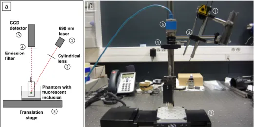
1 2 3 4 5 CCD detector 690 nm laser Phantom with fluorescent inclusion Emission filter Translation stage Cylindrical lens 1 2 3 4 5 a bFigure 1. Optical setup used during the study (schematic (a) and platform (b)).
Most of the elements of the optical setup (illustrated on figure 1) used for this study are based on a classical setup for reflectance molecular imaging. The light source is a 690 nm fibered laser (Intense HPD model 7404) which illuminates a tissue-like liquid phantom. Fluorescence images are acquired with a CCD camera (PCO Pixelfly VGA, 640x480 pixels images) for each position of the object which rests on a motorized translation stage. A cylindrical lens is used to focus the laser on the phantom along a line of width 1 mm which sets the translation steps at 1 mm to fully illuminate the phantom. A fluorescence filter (Semrock Razoredge 808 nm long pass filter) is placed in front of the camera to stop all excitation photons so as to detect a fluorescence signal.
All the liquid phantoms used in this study were made with the same recipe to obtain tissue-like optical properties with an absorption coefficient µa = 0.05 cm−1 and a reduced scattering coefficient µs′ = 10 cm−1.
The fluorescent inclusions are 1 mm diameter tubes containing 3 µM of Indocyanine Green encapsulated in lipid nanoparticles (LNP-ICG9) diluted in the same preparation as the phantoms to match background optical properties. We added different amounts of LNP-ICG to the phantom preparation to obtain different ratios of fluorescence to background fluorescence.
Plexiglass fluorescence emission spectrum for a 690nm excitation 0 500 1000 1500 2000 2500 3000 3500 4000 4500 700 750 800 850 900 950 1000 Wavelength (nm) S ig n a l (a .u .) (dimensions in mm) Ø 1,8 Ø18 ,46 Ø2 Ø1,6 Ø 1,4 Ø 1,2
Figure 2. Spatial position and dimension of the target (left) and its fluorescence emission spectrum for a 690 nm excitation (right).
Three different types of phantoms were used for this study:
• a single inclusion located at different depths ranging from 1 mm to 1 cm,
• a fluorescent resolution target depicted in figure 2 This target consists of plexiglass pieces (which fluores-cence emission spectrum is given on the right of figure 2) embedded in a circular phantom made of polyester resin with optical properties matching those of the liquid phantoms. The target is then immerged in a liquid phantom at depths ranging from 1 mm to 4 mm to test the improvements in resolution with depth, • two inclusions located at the same depths but with different absorption coefficient (this will be described
more precisely in the absorption correction part of this paper (§ 3.3)).
2.2 Image processing methods
The image processing method we will present relies on the assumption of relationship between the excitation and the autofluorescence signals defined as following10:
A
E = kr (1)
where E is the excitation, A is the autofluorescence, r is the distance and k is a proportionality coefficient. If the assumption is true, knowing the excitation profile could give us an insight on the autofluorescence profile. Simulations and experimental validations were performed to test this relationship, with simulations parameters chosen to match the experimental conditions.
Two types of simulations were performed to check the validity of our hypothesis: first with the Monte-Carlo method (with 106 photon counts) and also with the NIRFAST software11, 12 which is based on the diffusion approximation.
In both simulations, the medium is a homogeneous fluorescent one in a slab geometry with tissue-like optical properties.
To experimentally validate our hypothesis, measurements were acquired on a homogeneous autofluorescent phantom. Fluorescence and excitation images were acquired. As with the simulations, we studied the profiles ratios A/E for several increasing levels of autofluorescence.
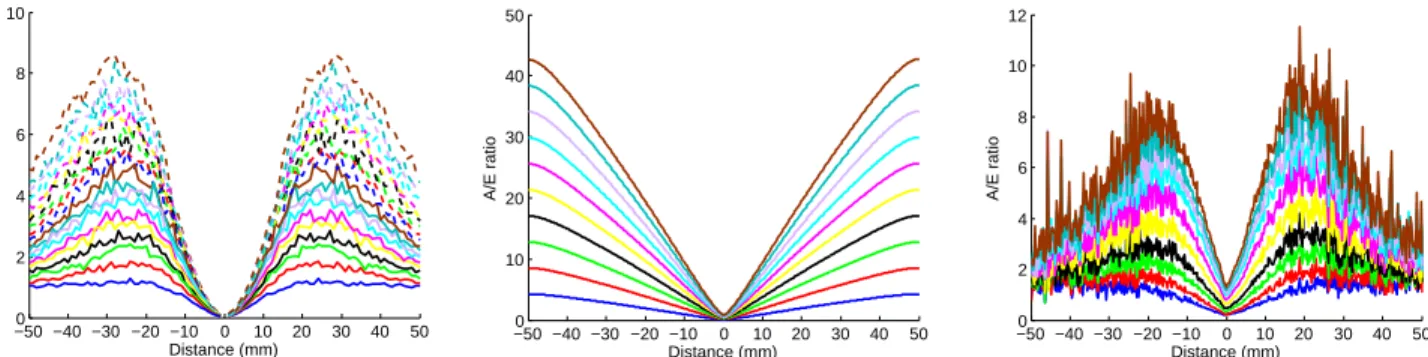
The results obtained with both simulations and experimentally are presented on figure 3.
−50 −40 −30 −20 −100 0 10 20 30 40 50 2 4 6 8 10 Distance (mm) A/E ratio −50 −40 −30 −20 −100 0 10 20 30 40 50 10 20 30 40 50 Distance (mm) A/E ratio −40 −50 −30 −20 −10 0 10 20 30 40 50 0 2 4 6 8 10 12 Distance (mm) A/E ratio
Figure 3. A/E intensity ratios obtained for increasing levels of autofluorescence with the Monte-Carlo method (left), with NIRFAST (center), experimentally (right).
A/E ratio profiles are presented for increasing levels of autofluorescence. We see the linear relationship of A/E with r for a distance inferior to 20 mm for both Monte-Carlo simulations and experimental acquisitions.
We suspect that their loss of linearity after this distance is due to the increase of noise due to the lack of photons. This linear relationship is even more visible on the simulations performed with NIRFAST as seen on the center of figure 3.
We will now explain how we take advantage of this relationship between the excitation and autofluorescence signals to reduce the effects of autofluorescence.
Let us consider that:
Itot≈ F + αE + A Itot≈ F + αE + βE.r
where Itot is the total signal detected on the camera, F is the fluorescence signal of interest, A is the autofluorescence, E are excitation leaks, α and β are coefficients.
By fitting Itotwith αE + βE.r, we can find the fluorescence signal of interest F by subtraction.
The fitting method is the following: for each excitation position, we acquire both a fluorescence and an excitation image. For each position, we then fit the fluorescence intensity profile in each column of the image by using the corresponding excitation profile with the method of least squares. We then obtain α and β parameters specific to each position. These parameters stay the same for excitation positions where only the autofluorescence is excited and have strong variations for positions surrounding the fluorescence target.
We studied two possibilities: we can either choose to use the parameters specific to each positions (referred as local parameters) or to use the mean parameters (referred as global parameters). As we will now see with the following simulations, each possibility has its own advantages and drawbacks.
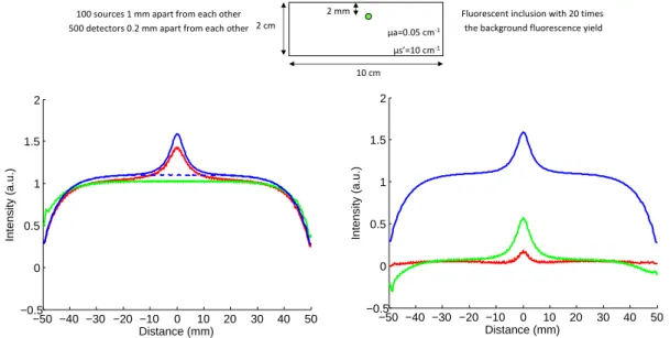
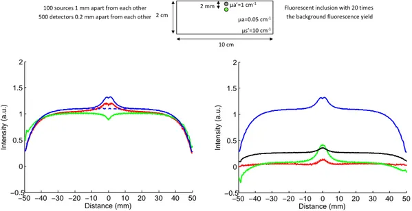
In the first case studied, we used the same medium as in the previous simulation and we added a fluorescent inclusion located 2 mm below the surface. The simulated phantom and the different intensity profiles of interest are depicted on figure 4.
µa=0.05 cm-1
µs’=10 cm-1
10 cm 2 cm
Fluorescent inclusion with 20 times the background fluorescence yield 2 mm
100 sources 1 mm apart from each other 500 detectors 0.2 mm apart from each other
−50 −40 −30 −20 −10 0 10 20 30 40 50 −0.5 0 0.5 1 1.5 2 Distance (mm) Intensity (a.u.) −50 −40 −30 −20 −10 0 10 20 30 40 50 −0.5 0 0.5 1 1.5 2 Distance (mm) Intensity (a.u.)
Figure 4. Intensity profiles comparison: left: —raw fluorescence F , - - -autofluorescence,—local
param-eters fit of the fluorescence M1, —global parameters fit of the fluorescence M2; right: —F , —(F − M1),
As expected, the intensity profile obtained when fitting with the local parameters is close to the total fluores-cence profile and is sensitive to the fluorescent inclusion, while the one obtained when using the global parameters is closer to the autofluorescence profile and is not sensitive to the fluorescent inclusion.
After subtraction, both methods completely nullify the autofluorescence contribution. The global parameters method leads to a better dynamic around the fluorescence inclusion but suffers from boundary effects.
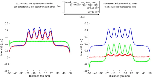
For the second case studied, we used the same medium as in the previous simulation and we added five fluorescent inclusions located 2 mm below the surface. The simulated phantom and the different intensity profiles of interest are depicted on figure 5.
1 cm 1 cm 1 cm 1 cm 1 2 3 µa=0.05 cm-1 µs’=10 cm-1 2 mm 10 cm 2 cm
100 sources 1 mm apart from each other
500 detectors 0.2 mm apart from each other 4 5
Fluorescent inclusions with 20 times the background fluorescence yield
−50 −40 −30 −20 −10 0 10 20 30 40 50 −0.2 −0.1 0 0.1 0.2 0.3 0.4 0.5 Distance (en mm) Intensité (u.a.) −50 −40 −30 −20 −10 0 10 20 30 40 50 −0.2 −0.1 0 0.1 0.2 0.3 0.4 0.5 Distance (en mm) Intensité (u.a.)
Figure 5. Intensity profiles comparison: left: —raw fluorescence F , - - -autofluorescence,—local
param-eters fit of the fluorescence M1, —global parameters fit of the fluorescence M2; right: —F , —(F − M1),
—(F − M2).
Contrary to the previous case where the parameters did not vary much and where taking their mean value allowed to get close to the background signal, in this case the parameters of the fluorescent objects vary more and have a bigger weight, leading to an overestimation of the autofluorescence when taking their mean value. This is why after subtraction we obtain a negative level of signal with the global parameters.
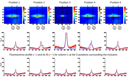
Figure 6 presents the behaviour of our model for five different positions of excitation around a fluorescent inclusion. It is possible to fit the autofluorescence signal with the excitation signal as the two profiles overlap when there is no fluorescence of interest. The differences between the two profiles that appear when there is some fluorescence signal of interest allow us to enhance this fluorescence signal by subtracting the fit to the whole fluorescence image.
To compare the different detection schemes and quantify the improvements, we use the contrast CT ,N defined as:
CT ,N =
hT i − hN i
hT i + hN i (2)
where hT i and hN i are respectively the mean intensity values in a target region of interest (with fluorescence) and in a neutral region of interest (with background fluorescence only).
Position 1 Position 2 Position 3 Position 4 Position 5
Fluorescence profile (―) and its fit (―) for column 1 at the 5 positions surrounding the inclusion
Fluorescence profile (―) and its fit (―) for column 2 at the 5 positions where there is only autofluorescence 1 2 1 2 1 2 1 2 1 2
1
2
Figure 6. Example of results obtained for 5 positions of the line surrounding a fluorescent inclusion.
3. RESULTS AND DISCUSSION
3.1 Contrast enhancement
We will first present the results obtained for the contrast in the case of a phantom with a single fluorescent inclusion at different increasing depths. Two different levels of background fluorescence were considered: a realistic one, and a stronger one to test the limits of the method.
On the left of figure 7, we compare the contrasts observed at the ten depths considered with the WF-FRI and both fitting methods for the realistic level of background fluorescence.
1 2 3 4 5 6 7 8 9 10 0 0.2 0.4 0.6 0.8 1 Inclusion depth (mm) Contrast (a.u.) 1 2 3 4 5 6 7 8 9 10 0 0.2 0.4 0.6 0.8 1 Inclusion depth (mm) Contrast (a.u.)
Figure 7. Comparison between the contrasts obtained with WF-FRI (—), the local parameters fitting
method (—) and the global parameters fitting method (—) for a realistic background fluorescence level
(left) and a stronger background fluorescence level (right) used to test the limits of the method.
there is a single fluorescent inclusion, the global parameters method offers better performance as mentioned before: the gain obtained with the local parameters varies between 1.2 at 1 mm and 3.1 at 10 mm while it varies between 1.4 and 4.4 with the global parameters.
On the right of figure 7, we present the results in the same case as before but with a stronger background fluorescence signal.
Even in this case with a stronger background signal, our fitting method enhances the contrast compared to the WF-FRI with both the local and global parameters. However, the gain obtained is smaller than the one obtained in the case with less background signal.
3.2 Resolution enhancement
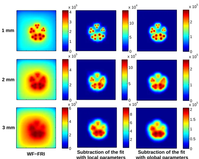
0 1 2 3 4 x 10⁵ 0 5 10 x 104 0 1 2 x 10⁵ 0 2 4 x 10⁵ 0 5 10 x 104 0 1 2 x 10⁵ 0 2 4 6 x 10⁵ 2 4 6 8 x 10⁴ 0 0.5 1 1.5 2 x 10⁵WF−FRI
1 mm
2 mm
3 mm
Subtraction of the fit
with local parameters
Subtraction of the fit
with global parameters
Figure 8. Images of the resolution target at three different depths obtained with WF-FRI (left column), the local parametes fitting method (central column) and the global parameters fitting method (right column). The second set of results was obtained with the fluorescent resolution target described in the previous part. The concentration of background fluorescence was set to have a realistic fluorescence to background ratio, and the target was immerged at three depths between 1 mm and 3 mm. The images obtained are presented on figure 8.
At 1 mm, it is possible to resolve the target with WF-FRI (left column) but there is already some crosstalk between the different groups of inclusions leading to an overestimation of the signal produced by the largest inclusions.
The local parameters fitting method (central column) offers the best performance. It enhances the reso-lution as it increases the peak to valley ratio between the fluorescent inclusions and the background, and the background fluorescence surrounding the inclusions is totally suppressed. The global parameters fitting method (right column) also suppresses the background fluorescence surrounding the inclusions, but the peak to valley ratio between the fluorescent inclusions and the background is slightly lower than with the local parameters fitting method.
At 2 mm, it becomes difficult to properly resolve the target with WF-FRI. Signals coming from the three largest groups of inclusions start to overlap and form one large fluorescent signal, making it impossible to distinguish the single inclusions in some groups.
The local parameters fitting method still offers the best performance as the resolution between the groups of inclusions is still good, but it becomes harder to see the inclusions in the group of inclusions with the smallest diameter. The global parameters fitting method gives results comparable to the ones obtained with the local parameters fitting method, but, as seen at 1 mm, the peak to valley ratio between the fluorescent inclusions and the background is slightly lower.
At 3 mm, the whole target only emits one large fluorescent signal with WF-FRI and the groups of inclusions are completely unresolved. With both fitting methods, the target is unresolved and we can only see one large signal due to the three largest groups of inclusions and two smallest signals due to the two smallest groups of inclusions.
3.3 Absorption correction
We first tested the absorption correction properties of our method in simulation with NIRFAST.
The first case studied (figure 9) is similar to the one presented on figure 4, but we added an absorbing heterogeneity juste above the fluorescent inclusion to deteriorate the detection with WF-FRI.
µa’=1 cm-1
µa=0.05 cm-1
µs’=10 cm-1
10 cm 2 cm
Fluorescent inclusion with 20 times the background fluorescence yield 2 mm
100 sources 1 mm apart from each other 500 detectors 0.2 mm apart from each other
−50 −40 −30 −20 −10 0 10 20 30 40 50 −0.5 0 0.5 1 1.5 2 Distance (mm) Intensity (a.u.) −50 −40 −30 −20 −10 0 10 20 30 40 50 −0.5 0 0.5 1 1.5 2 Distance (mm) Intensity (a.u.)
Figure 9. Intensity profiles comparison: left: —raw fluorescence F , - - -autofluorescence,—local
param-eters fit of the fluorescence M1, —global parameters fit of the fluorescence M2; right: —F , —(F − M1),
—(F − M2).
As previously mentioned, the profile obtained when using the local parameters is closer to the raw fluorescence profile while the profile obtained when using the global parameters is sensitive only to the absorption variation. After subtracting the profiles, the autofluorescence is correctly reduced with both fitting methods. We also can
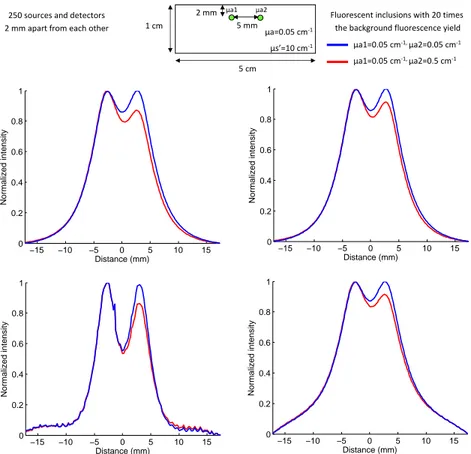
see that the drop in fluorescence observed in WF-FRI due to the absorbing heterogeneity is corrected. However, the fluorescence level is still lower than the one obtained for the simulation without the absorbing heterogeneity. The second case studied is a more complex one with two fluorescent inclusions at the same depths separated by 5 mm in the horizontal axis as depicted on figure 10.
µa=0.05 cm-1
µs’=10 cm-1
5 cm 1 cm
Fluorescent inclusions with 20 times the background fluorescence yield 2 mm
250 sources and detectors
2 mm apart from each other 5 mm
µa1=0.05 cm-1, µa2=0.05 cm-1 µa1=0.05 cm-1, µa2=0.5 cm-1 µa1 µa2 −15 −10 −5 0 5 10 15 0 0.2 0.4 0.6 0.8 1 Distance (mm) Normalized intensity −15 −10 −5 0 5 10 15 0 0.2 0.4 0.6 0.8 1 Distance (mm) Normalized intensity −15 −10 −5 0 5 10 15 0 0.2 0.4 0.6 0.8 1 Distance (mm) Normalized intensity −15 −10 −5 0 5 10 15 0 0.2 0.4 0.6 0.8 1 Distance (mm) Normalized intensity
Figure 10. Normalized intensity profiles with the same absorption coefficients (—) and different absorption
coefficients (—): top left: WF-FRI; top right: ratio method; bottom left: local parameters fitting method;
bottom right: global parameters fitting method.
Two simulations were performed: one where both fluorescent inclusions have the same absorption coefficient as the background, and another one where one of the inclusions has an absorption coefficient ten times higher. We can notice as mentioned in the paragraph concerning the resolutiuon enhancement that the best resolution is obtained with the local parameters fitting method, the two fluorescent peaks being better separated than with the WF-FRI. As for the previous case where there was an absorption heterogeneity above the fluorescent inclusion, there is a compensation of the absorption thanks to our fitting method and also with the ratio technique. With both of these techniques, the compensation is comparable, the signal from the inclusion with the higher absorption is increased compared to the signal obtained with the WF-FRI.
This has also been verified experimentally. We studied a phantom in the same configuration with two fluorescent capillaries at the same depth, the difference with the simulation is that the distance between the capillaries is 1 cm.
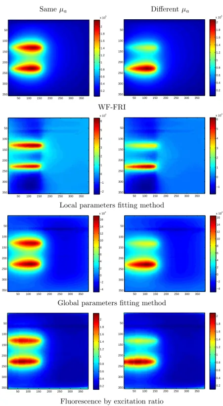
As for the simulation, two experiments were performed: one where both fluorescent inclusions have the same absorption coefficient as the background, and another one where one of the inclusions has an absorption coefficient ten times higher. The images obtained with the WF-FRI, both fitting methods, and the fluorescence to excitation ratio method are shown on figure 11.
Same µa Different µa 50 100 150 200 250 300 350 50 100 150 200 250 300 350 0.2 0.4 0.6 0.8 1 1.2 1.4 1.6 1.8 2 x 10⁵ 50 100 150 200 250 300 350 50 100 150 200 250 300 350 0.2 0.4 0.6 0.8 1 1.2 1.4 1.6 1.8 2 x 10⁵ WF-FRI 50 100 150 200 250 300 350 50 100 150 200 250 300 350 −2 −1 0 1 2 3 4 5 6 x 10⁴ 50 100 150 200 250 300 350 50 100 150 200 250 300 350 −1 0 1 2 3 4 5 6 x 10⁴
Local parameters fitting method
50 100 150 200 250 300 350 50 100 150 200 250 300 350 −4 −2 0 2 4 6 8 10 12 14 16 x 104 50 100 150 200 250 300 350 50 100 150 200 250 300 350 −4 −2 0 2 4 6 8 10 12 14 16 x 104
Global parameters fitting method
50 100 150 200 250 300 350 50 100 150 200 250 300 350 0.2 0.4 0.6 0.8 1 1.2 1.4 1.6 1.8 2 50 100 150 200 250 300 350 50 100 150 200 250 300 350 0.2 0.4 0.6 0.8 1 1.2 1.4 1.6 1.8 2
Fluorescence by excitation ratio
Figure 11. Images obtained with the different methods for two configurations: left: both capillaries have the same absorption coefficient; right: the top capillary has an absorption coefficient ten times higher.
As expected, the higher absorption of the top capillary leads to a decrease of its signal intensity it is twice as low as the one of the capillary having the same absorption as the background. The fact that the decrease of the intensity observed is higher experimentally than in simulation can be explained by the difference in distance between the capillaries: in simulation, the signals add more as the capillaries are closer, which diminish the
effects of absorption.
To have a quantitative idea of the absorption correction of the different techniques, we have plotted on figures 12 and 13 respectively the intensity profiles taken perpendicularly to the capillaries for the different methods, and the normalized intensity profiles. The results obtained experimentally are comparable to the ones obtained in simulation. −400 −30 −20 −10 0 10 20 30 40 0.5 1 1.5 2 2.5x 10 5 Distance (mm) Intensity (a.u.) −400 −30 −20 −10 0 10 20 30 40 0.5 1 1.5 2 Distance (mm) Intensity (a.u.) −40 −30 −20 −10 0 10 20 30 40 −4 −2 0 2 4 6 8x 10 4 Distance (mm) Intensity (a.u.) −40 −30 −20 −10 0 10 20 30 40 −5 0 5 10 15 20x 10 4 Distance (mm) Intensity (a.u.)
Figure 12. Intensity profiles with the same absorption coefficients (—) and different absorption coefficients
(—): top left: WF-FRI; top right: ratio method; bottom left: local parameters fitting method; bottom
right: global parameters fitting method.
−15 −10 −5 0 5 10 0 0.2 0.4 0.6 0.8 1 Distance (mm) Normalized intensity −10 −5 0 5 10 0 0.2 0.4 0.6 0.8 1 Distance (mm) Normalized intensity −10 −5 0 5 0 0.2 0.4 0.6 0.8 1 Distance (mm) Normalized intensity −10 −5 0 5 10 0 0.2 0.4 0.6 0.8 1 Distance (mm) Normalized intensity
Figure 13. Normalized intensity profiles with the same absorption coefficients (—) and different absorption
coefficients (—): top left: WF-FRI; top right: ratio method; bottom left: local parameters fitting method;
First, we can notice that the local parameters fitting method enhances the resolution compared to other methods. It also appears that no method totally corrects the effects of absorption. The difference with the simulation is that the only method that increases the signal of the higher absorption capillary is the local parameters fitting method: the signal is at 63 % of its original level, contrary to the other methods where it is at 50 %.
4. CONCLUSION
We presented in this paper a novel approach for molecular imaging based on the use of a laser line illumination rather than the more classical WF-FRI. By using a laser line to illuminate the object to study and acquiring fluorescence and excitation images for each position of the line, we can use the relationship existing between the excitation and autofluorescence intensity profiles to enhance the contrast and resolution of the signals.
While a strong background fluorescence can reduce the performance of the method, we can still expect a noticeable improvement compared to the WF-FRI. We also showed that this technique can be an alternative to the ratio method used by some groups to account for the absorption heterogeneities and correct the absorption effects. While we saw that in some cases the technique can totally correct these detrimental effects, there is still some work to be able to use this correction in all the cases of interest.
REFERENCES
[1] Frangioni, J. V., “In vivo near-infrared fluorescence imaging,” Current opinion in chemical biology 7, 626– 634 (Oct. 2003). PMID: 14580568.
[2] Ntziachristos, V., Bremer, C., and Weissleder, R., “Fluorescence imaging with near-infrared light: new technological advances that enable in vivo molecular imaging,” European radiology 13, 195–208 (Jan. 2003). PMID: 12541130.
[3] Sevick-Muraca, E. M., Houston, J. P., and Gurfinkel, M., “Fluorescence-enhanced, near infrared diagnostic imaging with contrast agents,” Current opinion in chemical biology 6, 642–650 (Oct. 2002). PMID: 12413549. [4] Hilderbrand, S. A. and Weissleder, R., “Near-infrared fluorescence: application to in vivo molecular
imag-ing,” Current opinion in chemical biology 14, 71–79 (Feb. 2010). PMID: 19879798.
[5] Demos, S. G., Gandour-Edwards, R., Ramsamooj, R., and White, R. d., “Near-infrared autofluorescence imaging for detection of cancer,” Journal of biomedical optics 9, 587–592 (June 2004). PMID: 15189097. [6] Paras, C., Keller, M., White, L., Phay, J., and Mahadevan-Jansen, A., “Near-infrared autofluorescence for
the detection of parathyroid glands,” Journal of Biomedical Optics 16(6), 067012 (2011).
[7] Shao, X., Zheng, W., and Huang, Z., “In vivo diagnosis of colonic precancer and cancer using near-infrared autofluorescence spectroscopy and biochemical modeling,” Journal of biomedical optics 16, 067005 (June 2011). PMID: 21721826.
[8] Han, X., Lui, H., McLean, D. I., and Zeng, H., “Near-infrared autofluorescence imaging of cutaneous melanins and human skin in vivo,” Journal of Biomedical Optics 14(2), 024017 (2009).
[9] Navarro, F. P., Berger, M., Goutayer, M., Guillermet, S., Josserand, V., Rizo, P., Vinet, F., and Texier, I., “A novel indocyanine green nanoparticle probe for non invasive fluorescence imaging in vivo,” 71900L– 71900L–10, SPIE (2009).
[10] Soubret, A. and Ntziachristos, V., “Fluorescence molecular tomography in the presence of background fluorescence,” Physics in medicine and biology 51, 3983–4001 (Aug. 2006). PMID: 16885619.
[11] Dehghani, H., Eames, M. E., Yalavarthy, P. K., Davis, S. C., Srinivasan, S., Carpenter, C. M., Pogue, B. W., and Paulsen, K. D., “Near infrared optical tomography using NIRFAST: algorithm for numerical model and image reconstruction,” Communications in numerical methods in engineering 25, 711–732 (Aug. 2008). PMID: 20182646.
[12] Jermyn, M., Ghadyani, H., Mastanduno, M. A., Turner, W., Davis, S. C., Dehghani, H., and Pogue, B. W., “Fast segmentation and high-quality three-dimensional volume mesh creation from medical images for diffuse optical tomography,” Journal of Biomedical Optics 18(8), 086007–086007 (2013).