Simulation of liquid-liquid interfaces in porous media

HAL Id: hal-01476939

https://hal-amu.archives-ouvertes.fr/hal-01476939

HAL is a multi-disciplinary open access archive for the deposit and dissemination of sci-entific research documents, whether they are pub-lished or not. The documents may come from teaching and research institutions in France or abroad, or from public or private research centers.

L’archive ouverte pluridisciplinaire HAL, est destinée au dépôt et à la diffusion de documents scientifiques de niveau recherche, publiés ou non, émanant des établissements d’enseignement et de recherche français ou étrangers, des laboratoires publics ou privés.

Simulation of liquid-liquid interfaces in porous media

Edder García, Pascal Boulet, Renaud Denoyel, Jérôme Anquetil, Gilles Borda,

Bogdan Kuchta

To cite this version:

Edder García, Pascal Boulet, Renaud Denoyel, Jérôme Anquetil, Gilles Borda, et al.. Simulation of liquid-liquid interfaces in porous media. Colloids and Surfaces A: Physicochemical and Engineering Aspects, Elsevier, 2016, 496, pp.28 - 38. �10.1016/j.colsurfa.2015.10.047�. �hal-01476939�

Simulation of Liquid-Liquid Interfaces in Porous Media

Edder J. GARCÍA1, PascalBOULET1, RenaudDENOYEL1, Jérôme Anquetil2, Gilles Borda3, BogdanKUCHTA1_*

1_{Aix-Marseille Université, CNRS, MADIREL, UMR 7246, 1339 Marseille France} 2_{TAMI-INDUSTRIES, 26110 Nyons, France}

3_{Commissariat Energie Atomique et Energies Alternatives, SGCS, Marcoules, France}

Highlights

 Incidence of porous membrane structure on the interface extent between two liquids has been studied

 The numerical model was generated by using the Lubachevsky-Stilliger algorithm.  The simulated annealing method was applied to minimize the energy of the liquid-liquid

interface

 A systematic study of the effect of the contact angle on the liquid-liquid interface has been performed.

 The contact angle and porosity are the most important properties controlling the extent of liquid-liquid interfaces.

Abstract

The properties of the interface of two immiscible fluids play an important role in several processes such as membrane supported liquid extraction, enhance oil recovery, aquifer remediation, etc. In this paper the spatial distribution of two immiscible liquids in non-dispersive contact via a porous media is studied by using numerical simulations. The simulations are carried at pore-scale by minimizing the total interfacial energy using the simulated annealing method. This technique allows us to compute the spatial distribution of fluids in the pores without assuming the geometry of the solid or the interface. The studied solids are made of randomly packed spheres either monodispersed or bi-dispersed. The effect of pore size distribution, tortuosity, porosity and contact angle on the liquid-liquid interface extent and geometry is analyzed. The simulations demonstrate that liquid-liquid interface follows a simple linear correlation with the contact angle. At low contact angle the wetting phase extents into the non-wetting phase forming pendular liquid bridges. The continuity of the phases is evaluated. The liquid-liquid interface is mostly continuous for all the contact angles.

KEYWORDS: simulated annealing, membrane, liquid extraction, pertraction, transport in porous media, partial wetting, contactors.

1. Introduction

Transport properties in porous media are subject of many studies in the context of various technological processes such as enhanced oil recovery, aquifer remediation, membrane separation, carbon sequestration, etc. Among the problems of interest are diffusion and its dependence on the multiphase equilibria of fluids penetrating porous structures. In particular, the liquid-liquid interfacial area is an important parameter for the mass transfer between the phases [1–5]. It is also important to describe the flow of liquids in the porous material.[6,7]

The interfacial area of two immiscible fluids inside a porous media can be measured by two main methods: 1) the interfacial tracer technique [8–11,11–15] and 2) high-resolution microtomography [16–18]. On the other hand, numerical simulations and theoretical models are useful to gain a better understanding of the shape and extent of the interface and its relationship with parameters as porosity, grain size and contact angle. There are several theoretical and empirical models in the literature to quantify the interfacial areas in porous media [18–22]. All these studies were carried out on systems where a phase is dispersed into the other, i.e. when coalescence is negligible. In this paper we are interested in interfaces between two liquids in contact inside a porous material separating the two immiscible phases. This non-dispersive contact can be found in several technological processes such as membrane supported liquid-liquid extractions [23–27], the so-called pertraction, aquifer remediation [28], and the immiscible displacement of oil [29–31]. In the pertraction process the porous material plays the role of immobilizing the interface across which the mass transfer takes place. A complete kinetic model for these systems should take into account the rate of transfer at the interface. The interface is mainly characterized by its location, shape, and extent which are controlled by capillary forces. Therefore, one can deduce that the properties of the solid affect the properties of the liquid-liquid interface. For that reason an important question is the following: to what extent the properties of the porous material and its wettability change the interfacial area? To the best of our knowledge, there are not hitherto studies describing the relationship between the interface of two liquids in non-dispersive contact and the properties of the solid.

In systems governed only by interfacial forces the distribution of phases at equilibrium is given by the minimum in the total Gibbs interfacial excess free energy (Gmin). Due to the complex relationship between Gmin and the pore geometry it can be determined analytically only for a few simple pore geometries. Therefore, numerical methods are used in the case of complex pores. The

simulated annealing method has been proposed as a reliable method to find the distribution of phases in three-dimensional porous materials [32–36]. On one hand, it can be applied to all kind of porous networks without assuming the geometry of the interface or pores. Hence, a more realistic representation of the pores can be used. On the other hand, the main disadvantages of this method are its high demand of required memory and computational time. The goal of this paper is to study how textural properties of the solid and its wettability impact the liquid-liquid interface inside a porous matrix. In particular the porosity, grain size, size dispersion, pore size distribution (PSD), and tortuosity are taken into account. The spatial distribution of the phases is calculated by minimizing the total interfacial energy using the simulated annealing technique.

2. Porous media with fixed physical-chemistry properties

The properties of porous materials are defined by their tortuosity, porosity and grain size distribution, among others. The following section describes the algorithm used to generate a model of the solid and the methods used to characterize such solids.

2.1 Porous media generation

In order to simulate the interface of two immiscible fluids in a porous solid media a detailed model of the solid is needed. The role of this model is to provide an idealization of the real solid (porous membrane, soil, or tissue) preserving its characteristics. Ideally the model should capture all properties of the real random solid. Unfortunately most of porous solids are too complex for a complete and accurate description. In addition, a general procedure to carry out reconstructions of disordered structures is possible only for some random media [37]. In this paper, as a first step, the porous material is represented as a dense packing of monodispersed or bidispersed spheres. This is an idealization of a real porous solid, but it provides a simple model that allows us to study the relationship between some relevant properties, such as the PSD, tortuosity, porosity, and the interfacial area. Another option is to use extended experimental reconstructions of natural media [33].

The algorithm to generate the random packing of spheres is based on the Lubachevsky-Stillinger protocol [38,39]. In this algorithm, the porosity and the grain size distribution are set to a desired

target. First, all spheres centers are randomly located in the simulation box. Then, the spheres are allowed to grow using a pre-specified rate. The eventual collision between spheres are solved using a repulsive hard-core potential. The growing of spheres is stopped when the system reaches the pre-specified porosity and size grain distribution. In this paper two particle size distribution are used as solids: monodisperse and bidisperse systems. For the bidisperse packing, the radius of the smallest spheres is half the radius of the largest ones. An example of simulation box of monodisperse and bidisperse spheres is shown in Figure 1A and B, respectively.

The structures are transformed into 3-D binary matrix by dividing the unit cell into smaller cages called voxels (or bins). For all the calculations carried out in this paper the cubic simulation box is divided into 150 parts in each direction of space. Thus, 1503 voxels (or bins) are formed. The following convention is used: voxels that belong to the solid phase are marked as 1, while those that are part of the porous space are marked as 0. To guarantee a sufficiently high resolution the smallest sphere diameter is always greater than 10% the length of the simulation box. Thus the minimum sphere diameter is equal to 15 voxels. The maximal sphere diameter is equal 35 voxels. As a consequence, the volumes of a sphere is always below 1.5% of the total box volume.

Randomly packed grains can have a wide variety of pores with different geometries. In order to have a correct representation of such pores and to calculate the average properties of the solid discussed below, such as its tortuosity, PSD and the liquid-liquid interface, M packings of grains with the same porosity and grain size distribution are generated. The number M is set to be representative of all possible configurations for the specific porosity and grain size distribution.

2.2 PSD calculations

The PSD is calculated using the distance transform of the binary matrix. A distance transform or distance map of a binary map is a matrix containing the distances between the nearest voxel belonging to a different phase [40]. The calculation is performed only for the phase of interest, i.e. for the porous phase. In order to reduce the computational cost, a spherical cutoff radius is applied. Thus, only voxels inside the spherical cutoff are taken into account. The cutoff radius used here is equal to half the length of the cubic simulation box. Periodic boundary conditions are used in the three dimension of space.

The cumulative pore volume (CPV) is calculated by inserting in each voxel spheres of radius r. The insertions start from the largest sphere to the smallest ones. The distance transform is used to

localize voxels that allows the algorithm to insert a sphere of radius r without overlapping with the solid phase. Once a free place is found the space is occupied and the fraction of the porous space filled by the spheres is calculated. The pore size distribution is the negative value of the derivative of the pore volume with respect to the radius r (-dV(r)/dr) [41,42]. Due to the finite size of the voxels the pore volume is not continuously filled, hence this produces small jumps in the CPV which are amplified by the derivative. To avoid this effect the CPV curves are interpolated by using the spline method.

Since the simulation box have a finite size, it is not representative of all pores that would be present in a real porous solid with the same porosity and grain size distribution. To overcome this problem, the CPV and PSD are calculated for a large number of different simulation boxes with the same porosity and grain size distribution. Then, the average of the properties of all the packings is calculated. Successive grain packing are added until a converged PSD is obtained. The reduced porous radius (r*) used here is defined by: r* = r/L, where r is the porous radius and L is the length of the cubic simulation box. The method has been validated by using solids with a well-known PSD, e.g. cylindrical pores.

2.3 Tortuosity calculations

The tortuosity is defined as the ratio of the diffusivity in a free medium to the diffusivity in a porous material. It characterizes the sinuosity and interconnection of a given porous media. In this work the tortuosity (τ) was calculated by using the random walk method [43,44]. This method can be applied straightforwardly in the case of binary three-dimensional solids. In this method a “walker” is introduced in the pore space (voxels marked as 0) and a counter called time (t) is initialized (t = 0). Then one of its six nearest neighbors is chosen randomly. The walker jumps to the next position only if the chosen voxels belongs to the porous space, otherwise the jump is not carried out and a new neighbor is chosen. The counter t is incremented by 1 at every trial. For every t the squared distance is calculated from the starting point. This calculation is repeated for a pre-established number of trials (Maxstep). Here Maxstep is set at 50.000 trials. Once Maxstep is reached a new walker is introduced at a random location. The mean square displacement at each t for several walkers is calculated by:

〈𝑟2_{〉 =} 1

𝑘𝑡𝑟𝑦∑ 𝑟𝑖2

𝑘𝑡𝑟𝑦

𝑖=1

(1)

where ktry is the number of walkers. The tortuosity is calculated at each t is given by: 𝜏 = 〈𝑟

2_{〉(𝑓𝑟𝑒𝑒 𝑠𝑝𝑎𝑐𝑒)}

〈𝑟2_{〉(𝑝𝑜𝑟𝑜𝑢𝑠 𝑚𝑒𝑑𝑖𝑎)}

(2)

To improve the statistic new walkers are continuously added. The simulation finishes when the relative error calculated by equation (3) falls below 0.01%.

𝑒𝑟 =|𝜏𝑜𝑙𝑑 − 𝜏𝑛𝑒𝑤| 𝜏𝑛𝑒𝑤 𝑥100

(3)

As in the case of the PSD, the mean tortuosity for a given porosity is calculated for a large number of randomly distributed spheres packing (M).

3. Methodology to determine the interfacial area

Consider a porous solid that is brought into contact at one side with a wetting liquid (liquid 1, L1) and a non-wetting liquid (liquid 2, L2) at the other side. Pressures pL1 and pL2 are applied to the wetting phase and non-wetting phase respectively. The porous space is completely filled by the wetting fluid due to capillary forces. The non-wetting phase stays out of pore space until pL2 reaches the threshold pressure, pc. For cylindrical pores pc is calculated by the Young-Laplace

equation:

𝑝_𝐿2− 𝑝_𝐿1 = 𝑝_𝑐 = 2𝛾𝑐𝑜𝑠𝜃 𝑟

(4)

where γ is the liquid-liquid surface tension, θ is the contact angle, and r is the radius of the cylindrical pore. If the system is isothermal, reversible, with incompressible liquids, and with constant mass, the external work done on the interface is equal to the total interfacial free energy (G) and the volume displaced (ΔV) is given by:

−𝑝𝑐∆𝑉 = ∆𝐺 (5)

Finally at equilibrium ΔG = 0. Thus, an interface is created between the liquids in the porous solid. The bulk of the liquids are in non-dispersive contact, i.e. they do not disperse into each other. The interface is immobilized by the pressures pL2 and pL1, and the capillary forces. The capillary forces are determined by the surface tension, the contact angle, and the local geometry of the

porous solid. Thus, the distribution of phases and therefore the shape of the meniscus are functions of these parameters.

For a system governed by the total interfacial free energy, the equilibrium phase distribution inside a porous media is determined by the minimal interfacial energy. This minimum depends on the structure of the solid and several properties of the solid and liquids such as the contact angle and the surface tension. Due to the complex relationship between the properties of the interface (i.e. shape, extent, and location) and the properties of the solid, the minimum, and therefore the distribution of the phases at equilibrium, can only be determined by numerical methods [32,45,46]. A common method used to determine the minimal interfacial energy is the simulated annealing technique [32–36]. It is usually applied to solve a variety of general problems relating to finding a state of minimum ‘‘energy’’ among a set of many local minima. Standard annealing methodology has been defined by using a control parameter T and the Boltzmann probability distribution [33,45]. If the system is carefully annealed then it reaches the minimum energy state. For a system where the interfacial energy is dominant, the physically relevant parameter is the total interfacial free energy. This means that the effect of all other forces such as gravity can be neglected. Thus, the target function to be minimized is:

𝐺 = ∑ 𝐴_𝑖𝛾_𝑖

𝑖

(6)

where Ai and γi are the interfacial area and the surface free energy of the interface i. For a system with three pure phases three interfaces are formed. Thus, considering a system made of liquid 1 (L1), liquid 2 (L2), and the solid (S) the interfaces are L1L2, L1S, and L2S, and G is given by:

𝐺 = 𝐴𝐿1𝐿2𝛾𝐿1𝐿2+ 𝐴𝐿1𝑆𝛾𝐿1𝑆+ 𝐴𝐿2𝑆𝛾𝐿2𝑆 (7)

The relationship between the free surface energies and the contact angle (θ) is given by Young’s equation:

𝛾_𝐿1𝑆 = 𝛾_𝐿2𝑆− 𝛾_𝐿1𝐿2𝑐𝑜𝑠𝜃 (8)

Substituting equation (8) into (7) and rearranging gives:

Note that the last term in equation (9) is the total surface area of the solid (As), AS = AL1S + AL2S. Therefore, it is a constant. Differentiating the total interfacial energy yields:

𝛥𝐺 = 𝛾_𝐿1𝐿2(𝛥𝐴_𝐿1𝐿2− 𝛥𝐴_𝐿1𝑆𝑐𝑜𝑠𝜃) (10)

To apply the annealing method the simulation box is divided into N voxels. As stated previously, voxels marked as 0 can be occupied by liquid 1 or 2 (pore media), while bins marked as 1 are part of the solid and cannot be occupied by any liquid. At the beginning all the pore space is filled randomly by liquid 1 or liquid 2 until a given volume ratio L1/L2 is reached. The ratio L1/L2 defines the wetting phase saturation (Sw). To study the effect of the contact angle Sw was fixed at 0.5. The choice of this value is justified in section 4.4.

The objective here is to find the optimal location of bins of liquids 1 and 2 that gives the global minimum in G. To start a simulation two bins of liquid 1 and liquid 2 located at the interfaces L1L2, L1S, or L2S are randomly selected and exchanged. The change in the total interfacial free energy is calculated using equation (10). If ΔG ≤ 0 the new configuration is accepted. On the other hand, if G>0 the probability to accept the new configurations is calculated by:

𝑃 = 𝐸𝑥𝑝 (− ∆𝐺 𝐺_𝑟𝑒𝑓)

(11)

where Gref is an arbitrary reference energy. It is analogous to the product of the temperature (T) with the Boltzmann constant (k) in the Metropolis Algorithm [47]. The “uphill” configurations allow the system to avoid being trapped in a local minimum. The random exchange preserves the volume ratio L1/L2. The initial Gref is chosen to give an acceptance ratio greater than 0.8 [46,48]. Successive new configurations are proposed until the system reaches equilibrium. The average G of accepted configurations over a large number of trials, called blocks, is used as equilibrium criteria. If the difference in <G> for two consecutive blocks is less than 0.1% the system is considered at equilibrium. The size of the blocks must be large enough to be representative of the system. The size of the block used here is >5x106_{. This guarantees that all locations in the pore}

media can be reached by both phases. In order to accelerate the convergence toward the equilibrium state only interfacial voxels are exchanged. The final results are not affected by this method since the blocks are large enough to allow that all the pore space is accessible to both phases.

A “cooling schedule” is chosen to reduce Gref so as to avoid trapping in local minima. Here, Gref is slowly reduced at a rate of 0.01%. The process is repeated for a large number of Gref. When the system approaches the global minimum the acceptance ratio converges to zero. The simulation finishes when the acceptance ratio for a block is lower that a given tolerance value. The tolerance value used here is 1x10-6_{. Several initial conditions of the system have been tested, showing no}

effect of the initial configuration on the final results.

To avoid border effects periodic boundary conditions (PBC) are used in the direction of axis x and y, while in the z direction the solid is always in contact with liquid 1 in +z and liquid 2 in –z. By taking these boundary conditions the system is analogous to an infinite layer of solid in contact with an infinite reservoirs of liquid 1 and liquid 2. These reservoirs are used only to simulate the contact of the solid with the bulk of the liquids. There is not exchange of mass between the reservoir and the simulation box. Thus, the system is closed. These PBC guarantee that the system evolves to a non-dispersive contact. As a convention the wetting fluid is always liquid 1 whereas liquid 2 is the non-wetting fluid.

By assuming that each bin face has an area equal to 1, the total interfacial area is calculated by counting the number of voxels in each interface.

It is worth mentioning that in previous works[32–36] ΔG is calculated by taking: ΔG = G2-G1, where G is given by Equation (7) and the superscripts 1 and 2 denote the state 1, before the change, and the state 2, after the change. By using this method all the interfacial energies must be known. Equation (10) depends only on the liquid-liquid interfacial energy, the contact angle and the change in the L1-L2 and L1-S interfacial area. This is advantageous because γL1L2 and the contact angle can be measured more easily than γL1S and γL2S.

Since the surface free energies are always positive, one can deduce from equation (10) that in order to minimize G the system tends to increase AL1S while AL1L2 is reduced. The contact angle determines the relative importance of AL1S with respect to AL1L2 on the total interfacial energy. Thus for θ = 0° both surfaces are equally weighted while for θ = 90° only AL1L2 is taken into account.

It is important to note that γL1L2 is a constant factor in Equation 10. Therefore the choice of γL1L2

does not affect the position of the minimum in G. This minimum is governed by the contact angle and the geometry of the interface. The value of γL1L2 used in this work is 11 mJ/m2.

4. Results

4.1 Characterization of porous media: PSD and tortuosity

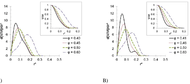
The PSD for randomly packed monodisperse and bidisperse spheres are shown in Figure 2 with respect to the pore radius.

Figure 2 shows that the average pore radius depends on the porosity. The solids with the lowest porosity have the smallest pore radius. In addition, it is clear that higher porosity leads to broader PSD while a low porosity produces a narrow peak. Similar results have been reported for packed monodisperse spheres by using theoretical models and experiments [49,50]. For φ = 0.40 a slight preference toward the formation of smaller pores is observed in the case of bidispersed spheres. This is caused by the smallest particles which tend to occupy more efficiently space forming smaller channels. For this low porosity a second peak appears for larger pore-sizes. Under this condition like, BCC-like and simple cubic-like (SC) clusters are formed. BCC-like and FCC-like structures give rise to smaller pores than SC-FCC-like. BCC and FCC are preferably formed, nevertheless some SC unit can be generated. For higher porosities the PSD are quite similar for monodispersed and bidispersed spheres.

Tortuosity is one of the important structural characteristics because it directly affects diffusion. At the same time, tortuosity depends critically on porosity which is a direct structural feature. Figure 3 shows the tortuosity for several grain configurations. In addition to randomly packed grains, face-centered cubic (FCC) and body-centered cubic (BCC) cubes and sphere cells were used as model in the calculation of the tortuosity. In order to generate low porosities the grains in FCC and BCC configurations are allowed to overlap. Figure 3 shows the tortuosity as function of the porosity. The following analytical model found in the literature [51–53] is used in Figure 3 to calculate the tortuosity :

𝜏 = 1 − 0.49𝑙𝑛(𝜑) (12)

We can see from Figure 3 that the tortuosity is strongly affected by the porosity. In addition, it is slightly dependent on the shape of the grains forming the porous network. The tortuosity for randomly packed spheres is in good agreement with equation 12. Figure 3 shows that randomly packed spheres have a higher tortuosity than FCC and BCC spheres but it is definitely lower than

FCC and BCC cubes. The observed divergence of the tortuosity at low porosity is the effect of the strong pore blocking when the wall building units are big.

A rapidity increase in tortuosity is observed when the particles start to overlap. The increase is significantly higher for FCC spheres. The coordination number of each sphere in FCC lattice is 12 while for BCC is 8. Therefore, FCC spheres can occupy more efficiently the space than BCC spheres. Thus, when the spheres overlap BCC lattices generate paths with fewer obstacles for the diffusing species. This means that diffusion of the random walkers is more hindered in the FCC lattice. Equation12 fail to describe this behavior since it was deduced for the case of random packed spheres.

4.2 Interface properties from free energy minimization

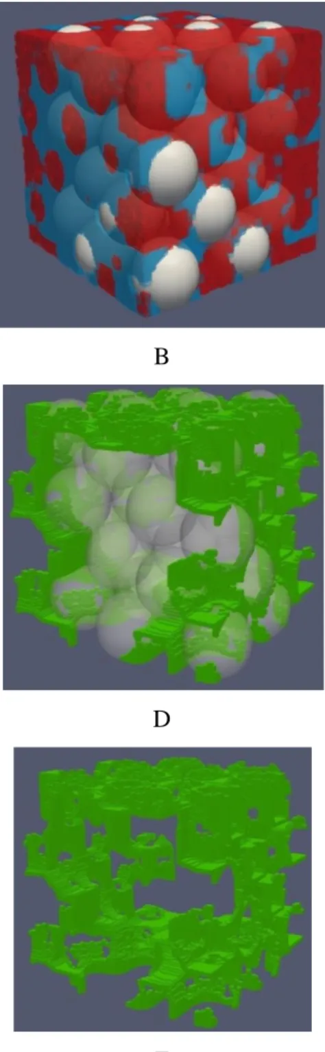
The distribution of phases and liquid-liquid interface for randomly packed monodisperse spheres with φ = 0.40 are shown in Figure 4. Also, a two-dimensional cut in the plane x-z of the spatial distribution of phases is shown in Figure 5. When the angle is equal to 90° the phases tend to separate so as to reduce the contact area between the liquid phases. In other words, the non-wetting phase is forced to stay in one side of the unit cell while the wetting phase is in the other side, where their respective reservoirs remain (Figure 4A). They form an almost flat interface (Figure 4F). The deviation from the strictly flat interface is due to the tortuosity of the porous solid. The interface follows the space available in the pores to bring into contact the phases. From the two-dimensional images (Figure 5A) it is clear that for this angle of 90° the interface is placed in the narrower pores. On the other hand, when the contact angle is zero it can be seen that the wetting zone is more dispersed to form large areas where the liquids are in contact (Figure 4B). The non-wetting fluid is located at the center of the larger pores (Figure 5B). The wetting phase increases the contact with the solid and at the same time increases the interface with the non-wetting phase. From the two-dimensional images it can be seen that thin layers of the wetting fluid enter into the non-wetting fluid in order to increase the contact surface with the solid. It is the formation of such layers or “fingers” that increases the liquid-liquid interface (Figure 5B). The fingers have the shape of pendular liquid bridges. It can be seen from Figure 5B that a single sphere can form multiple pendular liquid bridges. These structures have been experimentally observed in two phase systems [54–56].

All the narrow pores are occupied by the wetting phase as they offer the largest contact with the solid, then generating the lowest contact with the non-wetting phase. Hence the lowest interfacial energy is reached by filling such small pores with the wetting liquid. This is a well-known effect of capillary forces. In general, it can be seen that the liquid-liquid interfacial area increases as the contact angle decreases. In the following section a quantitative analysis of such variation is carried out.

Let us define the directionless liquid-liquid interfacial area A* as follows: A* = AL1L2/As, where

AL1L2 is the interfacial area of the liquids and As is the cross-sectional area of the simulation box.

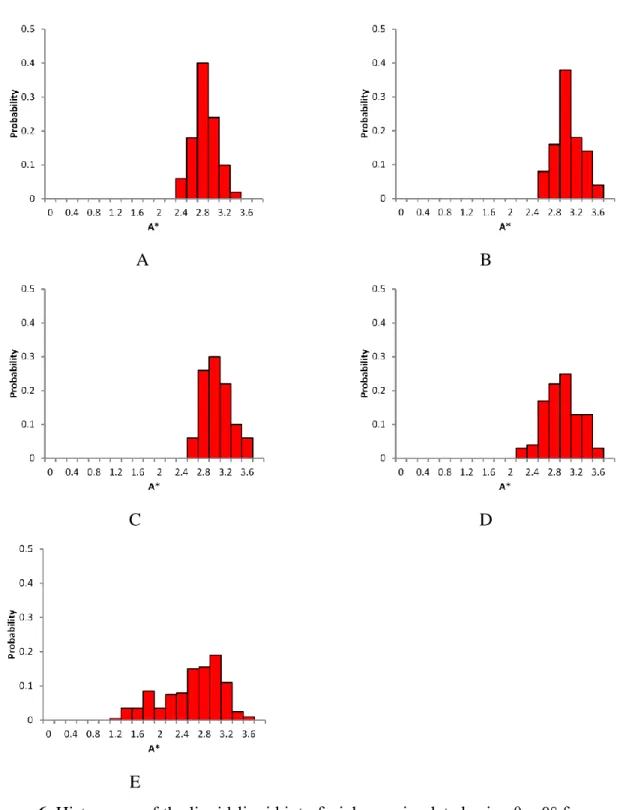
As stated before, in order to have a realistic representation of all pores for a given porosity and grain size distribution an ensemble of 50 packing structures is used when φ is lower than 0.8 and 200 for those with φ = 0.80. The histograms of the liquid-liquid interfacial area using θ = 0° for such sets of structures is shown in Figure 6.

It can be noticed that the distribution of A* gets narrower as the porosity decreases. This is because packing structures with low porosity have a narrow PSD. Therefore, most of the structures has similar pore size which leads to a narrow distribution of the liquid-liquid interfacial area. Figure 7 shows (average) A* as a function of the contact angle for monodisperse and bidisperse spheres.

It can be seen that A* is a close to a linear function of θ for all the porosities. A similar linear correlation is found for both cases: bidisperse and mononisperse spheres. When the contact angle is 90° the reduced area (A*) is close to the porosity. On the other hand, when liquid 1 completely wet the solid (contact angle = 0°) the liquid-liquid interface is approximately 2.8 times the cross sectional area of the solid.

4.3 Relationship between the liquid-liquid interface and the solid properties

Figure shows a plot of the interfacial area as a function of the porosity for several contact angles. It is observed that both monodisperse and bidisperse packings behave similarly. For small angles the plots show a maximum. The position of the maximum in interfacial area is governed by the contact angle. For small angles the peak is placed at low porosity while for larger angles it is placed

at higher porosities. If the contact angle is equal to 90° A* is linear function of the porosity. Bidispersed spheres have a slightly higher interfacial area than monodispersed grains. These observations can be explained as follows.

For small contact angles the wetting phase form pendular liquid bridges. Hence, the maximal L1/L2 interfacial area is given by the porosity that leads to the formation of a larger number of pendular liquid bridges with large size and curvature. The length of the fingers is mainly controlled by the free space between the spheres while the curvature is controlled by the contact angle and the gap between the spheres.[19,22] Thus, structures with low porosity, which have small pores, tend to form shorter fingers. The length of a pendular liquid bridge is limited by the balance between the free energy in the wetting phase-solid interface and the liquid-liquid interface. The former tends to decrease the energy while the later increases it. These fingers exist only for pore sizes that permit to decrease the energy. Thus, it is unlikely to form pendular liquid bridges with curvature radius significantly larger that the radius of the solid’s grain. This balance explains the maximum in the Figure .

The formation of multiple liquid bridges on a single sphere favors A*. This effect increases the interfacial area in bidisperse packed spheres since these packings have a larger number of spheres per volume. Therefore, the number of fingers per volume is increased.

We can conclude that since the PSD and the tortuosity are fixed by the porosity for randomly packed spheres, the interfacial area in non-dispersive systems is mainly controlled by the contact angle and the porosity.

4.4 Continuity of the liquid phases

Liquid phases in pore media can form two kinds of structures: bulk liquids and unconnected clusters. The continuity of the phases in the pores is an important property regarding mass transport and conductivity between the phases. This is because only the sections of the interface connected with the bulk are useful to transport matter across it. Thus, the formation of unconnected clusters must be quantified.

In this work the “forest-fire” algorithm is used to determine the number and size of clusters from the spatial distributions of phases obtained from the simulated annealing algorithm. In this method a voxel of the non-wetting or wetting phase is randomly chosen to start the “fire”, the voxel is

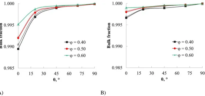
marked up as “burned”. Then, the “fire” is allowed to spread to all its 26 neighbors that belong to the same phase and that are not already marked up as “burned”. The new “burned” voxels are used to propagate the “fire” to its neighbors. The process is repeated until all the voxels in the cluster are reached. Then a new starting point is chosen from the voxels in the same phase which are not marked as “burned”. The calculation finishes when all the voxels in the phase are reached. PBC are used in x and y directions of space, while in z the liquid reservoirs are considered. Clusters in contact with its respective reservoir are considered as part of the bulk liquid phases while the other sections are unconnected clusters. The average fraction of the bulk liquids is calculated over the whole set of packing structures with same porosity. Figure shows the fraction of the bulk liquids as a function of the contact angle for monodisperse and bidisperse spheres.

Figure shows that continuous phases represent up to 98% of the phase for both monodisperse and bidisperse spheres. This means that the pendular liquid bridges formed in the wetting phase at low contact angle are connected. The formation of cluster decreases as the contact angle is increased. From these results we deduce that the meniscus of the bulk phases brings the main contribution to the liquid-liquid interfacial area. This result is quite different to that reported previously for the case of dispersive systems. For these systems the formation of liquid films (clusters of the wetting phase) is observed at low saturation.[21,33] The film or cluster configuration represent a small fraction of the phase in the case on non-dispersive contact. However, the formation of isolated clusters of the non-wetting phase is more important at low contact angle. This is because the formation of larger number of pendular liquid bridges at low θ can lead to segmentation of the non-wetting liquid. This mechanism is known as snap-off, and is favored by small pores.

4.5 Effect of the wetting phase saturation

The wetting phase saturation (Sw) is the fraction of the pore space occupied by the wetting liquid,

test the validity of the results for different saturation ratios.

Figure shows the liquid-liquid interfacial area for several saturations for packed monodisperse spheres with porosity equal to 0.40, the contact angle was fixed at 0°.

Figure shows that the interfacial area is constant in the range of saturation 0.1-0.5. It simply shows that, in the configuration adopted here, a variation of saturation is simply accompanied by the displacement of the interface in the pore matrix. For larger Sw A* decrease slightly. This result

is markedly different for that reported previously for the case of liquids in dispersive contact [19,22,33]. For these systems a maximum value of the interfacial area is reached when Sw is in the

range 0.2-0.3. The fall in A* for higher values of Sw is explained by a reduction of the space

5. Model interpretation

Wettability and porosity clearly controls the interfacial area between the liquids. We have shown that the interfacial area is a linear function of the contact angle. The increase in interfacial area with the contact angle has been reported in dispersive systems by using experimental measurements [57,58]. The interface brings into contact the liquids with the smallest possible liquid-liquid interfacial area. This is because by increasing this area the interfacial free energy is increased. On the other hand, the wetting phase – solid interface reduces the free energy, the amount of the reduction being proportional to the cosine of θ. Thus, by reducing the contact angle the interface is deformed to reach a larger fraction of the surface of the solid with the smallest L1/L2 interfacial area. Pendular liquid bridges are the structures formed by the wetting phase. This saddle-shaped interface permits the wetting phase to reach a larger surface of the solid with a minimal liquid-liquid interface. This guarantees that the phase distribution at equilibrium corresponds to the state of minimal interfacial energy.

In the case of non-dispersive contact the interfacial area can be several times as large as the cross sectional area of the solid for low angles. If for a given process the rate-limiting step is the transport, reaction, or adsorption of species at the interface the process can be speed up by reducing θ. Thus, by changing the nature of the fluids or the solid the interfacial area can be increased leading to an enhancement of the overall rate. The nature of the solid can be changed by surface modification. A lower angle is achieved when the polarity difference between the liquids is increased and the affinity toward the wetting liquid increases. On the other hand, according to equation 4 by reducing the contact angle the threshold pressure is increased. This is second beneficial effect since this means that the interface is more stable, thus a higher pressure differential can be applied. The main disadvantage of reducing the contact angle is the formation of isolated clusters in the non-wetting phase. This effect can lead to a loss of this phase into the wetting phase.

The structures studied in this work are simple randomly packed grains, however the method used here can be applied to any three-dimensional reconstructed network. Real porous material (membranes, soils, tissues, etc.) are more complex since they can be polydisperse, polymorph, have surface roughness, etc. These reconstructed models should capture better the geometry and size of the pores. Reconstructed three-dimensional models of real solids will generate more

realistic interfacial structures. Therefore, simulations on these systems will result in a better estimation of the liquid-liquid interface. A second simplification introduced in the simulations is the homogenous wettability of the solid. Real porous media can present heterogeneity in the chemical composition and surface roughness which can locally change the contact angle.

The simulations take into account only final equilibrium conditions of the system, while the imbibition-drainage displacements are not considered. These processes can lead to the dynamic change of the liquid-liquid interface.

6. Conclusions

In this work the effect of structural properties of porous solids on the interface between two liquids in non-dispersive contact has been studied. The presented results are for simple randomly packed spheres. These packed spheres were generated by using the Lubachevsky-Stilliger algorithm. In order to represent all the pores for a given porosity a large number of packing structures were taken into account. The simulated annealing method was applied to study the extent and geometry of the liquid-liquid interface. This method allows us to simulate the liquid-liquid interface without assuming the geometry of the pores. The simulation uses as input only the contact angle and the liquid-liquid interfacial tension which are more easily measured than the liquid-solid interfacial tension. It is important to mention that another modelling option is to use extended experimental reconstructions of natural media [33, 56]. However, it is much more computationally demanded and there are more parameters to control.

A systematic study of the effect of the contact angle on the liquid-liquid interfacial area has been carried out. The simulations have shown a linear correlation between the contact angle and interfacial area for the case of packed monodisperse and bidisperse spheres. This correlation can be used as a simple way to estimate the interfacial area, which is an important parameter in the mass transfer between the liquid phases and to scale-up non-dispersive systems. One example of this kind of system is a membrane contactor operated under partially wetted mode used in liquid-liquid extraction.

The contact angle is the main parameter controlling the geometry of the interface. Thus, for θ = 90° the interface is almost flat and parallel to the liquid reservoirs, while for θ = 0° it is curved. The wetting phase forms pendular liquid bridges while the non-wetting phase is located at the

centre of the larger pores. Thus, a larger and more tortuous interface can improve the probability of diffusing species to pass from one liquid to the other.

The PSD and tortuosity are fixed by the porosity for randomly packed spheres, thus the interfacial area is governed by the contact angle and the porosity. Nevertheless, there is a stronger dependence on the wettability than on porosity. The dispersivity of the grains size adds additional liquid-liquid interfacial area. However, its effect is small compared with the contact angle. Thus, we conclude that the contact angle and porosity are the most important properties controlling both the shape and the extent of liquid-liquid interfaces in porous media.

The structures of the liquid phases are mostly continuous. Therefore, the liquid-liquid interface is an uninterrupted pathway from one liquid to the other. The continuity of the liquid phases is an advantageous property regarding mass transfer. However, the non-wetting phase is slightly fragmented at low contact angle and low porosity, which can produce a loss (or dispersion) of the non-wetting phase into the wetting one.

ACNOWLEGEMENTS

This work has been supported by ANR-12-RMNR-03 MATEX grant of French National Research Agency (ANR)

7. References

[1] R.L. Detwiler, H. Rajaram, R.J. Glass, Interphase mass transfer in variable aperture fractures: Controlling parameters and proposed constitutive relationships, Water Resour. Res. 45 (2009) W08436. doi:10.1029/2008WR007009.

[2] M.L. Johns, L.F. Gladden, Magnetic Resonance Imaging Study of the Dissolution Kinetics of Octanol in Porous Media, J. Colloid Interface Sci. 210 (1999) 261–270.

doi:10.1006/jcis.1998.5950.

[3] R.J. Held, M.A. Celia, Pore-scale modeling and upscaling of nonaqueous phase liquid mass transfer, Water Resour. Res. 37 (2001) 539–549. doi:10.1029/2000WR900274.

[4] G.P. Grant, J.I. Gerhard, Simulating the dissolution of a complex dense nonaqueous phase liquid source zone: 1. Model to predict interfacial area, Water Resour. Res. 43 (2007) W12410. doi:10.1029/2007WR006038.

[5] H. Valdés, J. Romero, J. Sanchez, S. Bocquet, G.M. Rios, F. Valenzuela, Characterization of chemical kinetics in membrane-based liquid–liquid extraction of molybdenum(VI) from aqueous solutions, Chem. Eng. J. 151 (2009) 333–341. doi:10.1016/j.cej.2009.04.012. [6] W.G. Gray, S.M. Hassanizadeh, Unsaturated Flow Theory Including Interfacial

Phenomena, Water Resour. Res. 27 (1991) 1855–1863. doi:10.1029/91WR01260. [7] S.M. Hassanizadeh, W.G. Gray, Mechanics and thermodynamics of multiphase flow in

porous media including interphase boundaries, Adv. Water Resour. 13 (1990) 169–186. doi:10.1016/0309-1708(90)90040-B.

[8] M.L. Brusseau, J. Popovičová, J.A.K. Silva, Characterizing Gas−Water Interfacial and Bulk-Water Partitioning for Gas-Phase Transport of Organic Contaminants in Unsaturated Porous Media, Environ. Sci. Technol. 31 (1997) 1645–1649. doi:10.1021/es960475j. [9] K.P. Saripalli, P.S.C. Rao, M.D. Annable, Determination of specific NAPL–water

interfacial areas of residual NAPLs in porous media using the interfacial tracers technique, J. Contam. Hydrol. 30 (1998) 375–391. doi:10.1016/S0169-7722(97)00052-1.

[10] M.S. Costanza-Robinson, M.L. Brusseau, Air-water interfacial areas in unsaturated soils: Evaluation of interfacial domains, Water Resour. Res. 38 (2002) 1195.

[11] S. Peng, M.L. Brusseau, Impact of soil texture on air-water interfacial areas in unsaturated sandy porous media, Water Resour. Res. 41 (2005) W03021. doi:10.1029/2004WR003233. [12] H. Kim, P.S.C. Rao, M.D. Annable, Determination of effective air-water interfacial area in

partially saturated porous media using surfactant adsorption, Water Resour. Res. 33 (1997) 2705–2711. doi:10.1029/97WR02227.

[13] M.V. Karkare, T. Fort, Determination of the Air−Water Interfacial Area in Wet

“Unsaturated” Porous Media, Langmuir. 12 (1996) 2041–2044. doi:10.1021/la950821v. [14] K.P. Saripalli, H. Kim, P.S.C. Rao, M.D. Annable, Measurement of specific fluid-fluid

interfacial areas of immiscible fluids in porous media, Environ. Sci. Technol. 31 (1997) 932–936.

[15] L. Chen, T.C.G. Kibbey, Measurement of air-water interfacial area for multiple hysteretic drainage curves in an unsaturated fine sand, Langmuir ACS J. Surf. Colloids. 22 (2006) 6874–6880. doi:10.1021/la053521e.

[16] D. Wildenschild, C.M.P. Vaz, M.L. Rivers, D. Rikard, B.S.B. Christensen, Using X-ray computed tomography in hydrology: systems, resolutions, and limitations, J. Hydrol. 267 (2002) 285–297. doi:10.1016/S0022-1694(02)00157-9.

[17] G. Schnaar, M.L. Brusseau, Pore-Scale Characterization of Organic Immiscible-Liquid Morphology in Natural Porous Media Using Synchrotron X-ray Microtomography, Environ. Sci. Technol. 39 (2005) 8403–8410. doi:10.1021/es0508370.

[18] M.L. Brusseau, M. Narter, G. Schnaar, J. Marble, Measurement and Estimation of Organic-Liquid/Water Interfacial Areas for Several Natural Porous Media, Environ. Sci. Technol. 43 (2009) 3619–3625.

[19] H. Gvirtzman, P.V. Roberts, Pore scale spatial analysis of two immiscible fluids in porous media, Water Resour. Res. 27 (1991) 1165–1176. doi:10.1029/91WR00303.

[20] M. Oostrom, M.D. White, M.L. Brusseau, Theoretical estimation of free and entrapped nonwetting–wetting fluid interfacial areas in porous media, Adv. Water Resour. 24 (2001) 887–898. doi:10.1016/S0309-1708(01)00017-3.

[21] S.L. Bryant, A. Johnson, Bulk and film contributions to fluid/fluid interfacial area in granular media, Chem. Eng. Commun. 191 (2004) 1660–1670.

[22] E. Dalla, M. Hilpert, C.T. Miller, Computation of the interfacial area for two-fluid porous medium systems, J. Contam. Hydrol. 56 (2002) 25–48. doi:10.1016/S0169-7722(01)00202-9.

[23] A. Kiani, R.R. Bhave, K.K. Sirkar, Solvent extraction with immobilized interfaces in a microporous hydrophobic membrane, J. Membr. Sci. 20 (1984) 125–145.

doi:10.1016/S0376-7388(00)81328-9.

[24] N.S. Rathore, J.V. Sonawane, A. Kumar, A.K. Venugopalan, R.K. Singh, D.D. Bajpai, et al., Hollow fiber supported liquid membrane: a novel technique for separation and recovery of plutonium from aqueous acidic wastes, J. Membr. Sci. 189 (2001) 119–128.

doi:10.1016/S0376-7388(01)00406-9.

[25] P.K. Mohapatra, V.K. Manchanda, Liquid membrane based separations of actinides and fission products, Indian J. Chem. Sect. -Inorg. Bio-Inorg. Phys. Theor. Anal. Chem. 42 (2003) 2925–2938.

[26] A. Criscuoli, E.M.V. Hoek, V.V. Tarabara, Membrane Contactors, in: Encycl. Membr. Sci. Technol., John Wiley & Sons, Inc., 2013.

http://onlinelibrary.wiley.com/doi/10.1002/9781118522318.emst107/abstract (accessed August 25, 2014).

[27] P.K. Parhi, Supported Liquid Membrane Principle and Its Practices: A Short Review, J. Chem. 2013 (2012) e618236. doi:10.1155/2013/618236.

[28] K. Soga, J.W.E. Page, T.H. Illangasekare, A review of NAPL source zone remediation efficiency and the mass flux approach, J. Hazard. Mater. 110 (2004) 13–27.

doi:10.1016/j.jhazmat.2004.02.034.

[29] Y. Bai, J. Zhou, Q. Li, Stability analysis of the moving interface in piston- and non-piston-like displacements, Acta Mech. Sin. 24 (2008) 381–385. doi:10.1007/s10409-008-0161-2. [30] A.C. Payatakes, K.M. Ng, R.W. Flumerfelt, Oil ganglion dynamics during immiscible

displacement: Model formulation, AIChE J. 26 (1980) 430–443. doi:10.1002/aic.690260315.

[31] Y. Sugai, T. Babadagli, K. Sasaki, Consideration of an effect of interfacial area between oil and CO2 on oil swelling, J. Pet. Explor. Prod. Technol. 4 (2014) 105–112.

[32] R. Knight, A. Chapman, M. Knoll, Numerical modeling of microscopic fluid distribution in porous media, J. Appl. Phys. 68 (1990) 994. doi:10.1063/1.346666.

[33] B. Berkowitz, D.P. Hansen, A numerical study of the distribution of water in partially saturated porous rock, Transp. Porous Media. 45 (2001) 301–317.

[34] A.N. Galani, M.E. Kainourgiakis, N.I. Papadimitriou, A.T. Papaioannou, A.K. Stubos, Investigation of transport phenomena in porous structures containing three fluid phases, Colloids Surf. Physicochem. Eng. Asp. 300 (2007) 169–179.

doi:10.1016/j.colsurfa.2007.01.044.

[35] M.E. Kainourgiakis, E.S. Kikkinides, G.C. Charalambopoulou, A.K. Stubos, Simulated Annealing as a Method for the Determination of the Spatial Distribution of a Condensable Adsorbate in Mesoporous Materials, Langmuir. 19 (2003) 3333–3337.

doi:10.1021/la026766p.

[36] M.E. Kainourgiakis, E.S. Kikkinides, A. Galani, G.C. Charalambopoulou, A.K. Stubos, Digitally Reconstructed Porous Media: Transport and Sorption Properties, Transp. Porous Media. 58 (2005) 43–62. doi:10.1007/s11242-004-5469-1.

[37] M.D. Rintoul, S. Torquato, Reconstruction of the structure of dispersions, J. Colloid Interface Sci. 186 (1997) 467–476.

[38] B.D. Lubachevsky, F.H. Stillinger, Geometric properties of random disk packings, J. Stat. Phys. 60 (1990) 561–583. doi:10.1007/BF01025983.

[39] A.R. Kansal, S. Torquato, F.H. Stillinger, Computer generation of dense polydisperse sphere packings, J. Chem. Phys. 117 (2002) 8212. doi:10.1063/1.1511510.

[40] S. Jayaraman, S. Essakkirajan, T. Veerakumar, Digital Image Processing, Tata McGraw-Hill Education, 2011.

[41] P. Pfeifer, G.P. Johnston, R. Deshpande, D.M. Smith, A.J. Hurd, Structure analysis of porous solids from preadsorbed films, Langmuir. 7 (1991) 2833–2843.

doi:10.1021/la00059a069.

[42] L.D. Gelb, K.E. Gubbins, Pore Size Distributions in Porous Glasses:  A Computer Simulation Study, Langmuir. 15 (1999) 305–308. doi:10.1021/la9808418.

[43] Y. Watanabe, Y. Nakashima, RW3D. m: three-dimensional random walk program for the calculation of the diffusivities in porous media, Comput. Geosci. 28 (2002) 583–586.

[44] Y. Nakashima, T. Yamaguchi, DMAP. m: A Mathematica® program for three-dimensional mapping of tortuosity and porosity of porous media, Bull.-Geol. Surv. Jpn. 55 (2004) 93– 103.

[45] S. Kirkpatrick, C.D. Gelatt, M.P. Vecchi, Optimization by Simulated Annealing, Science. 220 (1983) 671–680. doi:10.1126/science.220.4598.671.

[46] S. Kirkpatrick, Optimization by simulated annealing: Quantitative studies, J. Stat. Phys. 34 (1984) 975–986. doi:10.1007/BF01009452.

[47] N. Metropolis, A.W. Rosenbluth, M.N. Rosenbluth, A.H. Teller, E. Teller, Equation of State Calculations by Fast Computing Machines, J. Chem. Phys. 21 (1953) 1087–1092. doi:10.1063/1.1699114.

[48] C.L.Y. Yeong, S. Torquato, Reconstructing random media, Phys. Rev. E. 57 (1998) 495– 506. doi:10.1103/PhysRevE.57.495.

[49] M. Alonso, E. Sainz, F.A. Lopez, K. Shinohara, Void-size probability distribution in random packings of equal-sized spheres, Chem. Eng. Sci. 50 (1995) 1983–1988. [50] V. Baranau, D. Hlushkou, S. Khirevich, U. Tallarek, Pore-size entropy of random

hard-sphere packings, Soft Matter. 9 (2013) 3361. doi:10.1039/c3sm27374a.

[51] Z. Sun, X. Tang, G. Cheng, Numerical simulation for tortuosity of porous media,

Microporous Mesoporous Mater. 173 (2013) 37–42. doi:10.1016/j.micromeso.2013.01.035. [52] M. Barrande, R. Bouchet, R. Denoyel, Tc, Anal. Chem. 79 (2007) 9115–9121.

doi:10.1021/ac071377r.

[53] H.L. Weissberg, Effective Diffusion Coefficient in Porous Media, J. Appl. Phys. 34 (1963) 2636. doi:10.1063/1.1729783.

[54] H. Gvirtzman, M. Magaritz, E. Klein, A. Nadler, A Scanning Electron Microscopy study of water in soil, Transp. Porous Media. 2 (1987) 83–93. doi:10.1007/BF00208538.

[55] R.T. Armstrong, M.L. Porter, D. Wildenschild, Linking pore-scale interfacial curvature to column-scale capillary pressure, Adv. Water Resour. 46 (2012) 55–62.

doi:10.1016/j.advwatres.2012.05.009.

[56] M. Han, S. Youssef, E. Rosenberg, M. Fleury, P. Levitz, Deviation from Archie’s law in partially saturated porous media: Wetting film versus disconnectedness of the conducting phase, Phys. Rev. E. 79 (2009) 031127. doi:10.1103/PhysRevE.79.031127.

[57] V. Jain, S. Bryant, M. Sharma, Influence of Wettability and Saturation on Liquid−Liquid Interfacial Area in Porous Media, Environ. Sci. Technol. 37 (2003) 584–591.

doi:10.1021/es020550s.

[58] C.J. Landry, Z.T. Karpyn, M. Piri, Pore-scale analysis of trapped immiscible fluid structures and fluid interfacial areas in oil-wet and water-wet bead packs, Geofluids. 11 (2011) 209–227. doi:10.1111/j.1468-8123.2011.00333.x.

A B

Figure 1. Examples of unit cells used as model of the solid: A) monodisperse spheres B)

A) B)

Figure 2. Pore size distribution for: A) monodisperse spheres B) bidisperse spheres. r* is the

reduced pore radius and  is the porosity. The reduced radius of the spheres is 0.20 for the monodisperse packing and 0.20 and 0.10 for the bidispersed packing.

A B

C D

E F

Figure 4. Interfaces in the case of monodisperse packed spheres (φ = 0.40) : Left column θ =

90°, right column θ = 0° . From top to bottom: spatial distribution of phases (blue = wetting liquid, red = non-wetting liquid), and liquid-liquid interface (in green).

A B

Figure 5. Case of monodisperse packed spheres (φ = 0.40) . Two dimensional cuts in the x-z

plane for A) θ = 90°and B) θ = 0°. Black = solid, gray = wetting liquid, and white: non-wetting liquid.

A B

C D

E

Figure 6. Histograms of the liquid-liquid interfacial area simulated using θ = 0° for several

(A) (B)

Figure 7. Liquid-liquid interfacial area as function of the contact angle for: A) monodisperse

Figure 8. Liquid-liquid interfacial area as a function of the porosity. Filled symbols:

A) B)

Figure 9. Fraction forming the bulk of the liquid as function of the contact angle for packed

monodispese and bidisperse spheres: A) non-wetting phase and B) wetting phase. Filled symbols: Monodisperse spheres; Open symbols bidisperse spheres.

Figure 10. Liquid-liquid interfacial area as function of the saturation for packed monodisperse