Design Optimization of Oxygenated Fluid Pump
by
Bruno Aiala Piazzarolo
Submitted to the
Department of Mechanical Engineering
in Partial Fulfillment of the Requirements for the Degree of Bachelor of Science in Mechanical Engineering
at the
Massachusetts Institute of Technology
June 2012
ARCHIVES
MASSACHUSETTS INSTITUTE OF TECHNOLOGYJUN
2
8 2012
L
BRARIES
© 2012 Massachusetts Institute of Technology. All rights reserved.
Signature of Author:
C-,
Department of Mechanical EngineeringMay 22, 2012
I-.---- ~
Certified by:
Alexander H. Slocum, PhD Neil and Jane Pappalardo Professo f Mechanical Engineering visor
John H. Lienhard V Samuel C. Collins P essor of Mechanical Engineering
Undergraduate Officer Accepted by:
Design Optimization of Oxygenated Fluid Pump
by
Bruno Aiala Piazzarolo
Submitted to the Deartment of Mechanical Engineering on May 22' in Partial Fulfillment of the
Requirements for the Degree of
Bachelor of Science in Mechanical Engineering
ABSTRACT
In medical emergencies, an oxygen-starved brain quickly suffers irreparable damage. In many cases, patients who stop breathing can be resuscitated but suffer from brain damage. Dr. John Kheir from Boston Children's Hospital created a compressible fluid that can re-oxygenate blood quickly in patients with asphyxia and cardiac arrest. Because the fluid is compressible, the set infusion rate on an ordinary pump does not necessarily indicate what is delivered. In addition, the fluid is provided at a 90% gas by volume concentration and is extremely viscous.
The goal of this project is to create a pump to deliver a specified volumetric flow rate of the oxygenated fluid created by the doctor. The pump design uses a bellows with force feedback calibration to pump 1 liter of fluid over 5 minutes and mix the concentrated 90% form with saline without degradation to form a 70% concentrated form with the viscosity similar to that of blood. My part in the project was to create the control system that would drive the pump using a force feedback and to optimize the design of the pump
The oxygenated fluid pump built can successfully store and dispense one liter of fluid, mix the concentrated form of the oxygenated fluid with saline, maintain sterility, and preserve the fluid's properties, all in a cost appropriate manner. It is a modular design that can easily be modified to improve its performance. Further testing is required to tune the control system and ensure that the flow rate is accurate to ±10%. The pump is mostly being used as a research tool in order to run tests that will help characterize the fluid and later can be used for small and large animal testing.
Thesis Supervisor: Alexander H. Slocum
AcKNOWLEDGEMENTS
I would first and foremost like to thank Professor Alex Slocum and teaching assistants/mentors Nevan Hanumara and Nikolai Begg for their expert advice, support and guidance in this project. I would also like to thank our clinician Dr. John N. Kheir, M.D for providing us with an exciting project that has tremendous potential to save lives.
I would also like to thank partners Alex Mason and Kristen Pena. We formed a team of extremely dedicated scholars determined to find a solution to the problem presented by our clinician. Without their support and wisdom this project would not have been successful.
Last but not least I would like to thank everyone who helped in the project in one way or another, mainly Lesley Yu (National Instruments representative for MIT) who provided great technical skills and support. She provided help with Labview to create the backbone of the control system used in this project. Thanks to Blow Molded Specialties, the Center for Bits and Atoms, 3-D Printsmith, and the MIT Hobby Shop for providing support with special parts and manufacturing needed for this project.
CONTENTS
A bstract ... 3
A cknow ledgem ents ... 5
C ontents ... 7 Figures ... 9 Tables ... 11 Chapter 1 ... 12 1.1 PURPOSE... ... 12 1.2 M OTIVATION ... ... ... ... .... .12 1.3 PUM P OVERVIEW ... ... o ... ... ... 13 1.4 PRIOR ART ... ... ... ... ... . . 15
1.4.1 Belmont Rapid Infuser ... 15
1.4.2 EnhancedACL Repair Gun ... 15
Chapter 2 ... ... 16 2.1 DESIGN REQUIREMENTS ... ... ... ... ... 17 2.1.1 Cost ... 17 2.1.2 Flow Rate ... 17 2.1.3 M ixing ... 18 2.1.4 Capacity ... 19 2.1.5 M edical-Specific Requirements ... 19 C hapter 3 ... 20
3.1 SYSTEM FLUID MODEL ... 20
3.1.1 Pressure ... 20
3.1.2 Resistances ... 22
3.2 PUM P DESIGN ... ... ... ... ... 25
3.2.1 Structure ... 26
3.2.2 Tubing and Connections ... 27
3.2.3 M otor and Load Cell Selection ... 28
3.2.4 Bellows ... 28
3.2.6 Volum e C alculation ... 31
3.2.7 Sliding M echanism ... 35
3.2.8 P eristaltic P um p ... 36
3.2.9 Static H elical M ixer ... 37
C hapter 4 ... ... 39 4.1 LOGIC ... 239 4.2 LAB iEW o n...42 4.2.1 Initialize . ... ... 42 4.2.2 Bellows Top ... .... ... ... . ... 3...5 4.2.3 M anual Jog ... 44 4.2.4 C alibration ... ... 46 4.2.5 M otor Control... 47 4.2.6 End...I Y .F . ... 49 Chapter 5 ... ... 50
5.1 FLOW RATE IE.I.T..UT ... ... ... 50
5.1.1 Peristaltic Pump ... 50 5.1.2 Bellow s Pump ... 51 5.2 PRIME TIME... 53 Chapter 6 .D O ... 54 6.1 QUALITY OF MIXING...54 6.2 VOLUME PERCENTAGE ... ... ... 54
6.3 PARTICLE SIZE DISTRIBUTION... . . ... -...- 57
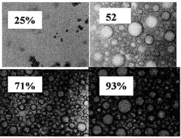
63.1 Microscopy (image for stratification) ... 59
6.4 OXYGEN TENSION... ... .. 61
6.5 R .EomETRY ... 62
6.6 DEGRADATION... ...-... 64
Chapter 7 ... ... 65
7.1 SUMMARY... .... --- ... ... o~o-o...6
References... . ... o... o.67 Appendix A ... ... 68
Appendix B... .. o...69
FIGURES
Figure 1.1: Overall System Diagram ... 14
Figure 2.1: Layout Of Fluid Path... 18
Figure 3.1: Layout Of Pump...21
Figure 3.2: Shear Stress Sweep ... 23
Figure 3.3: Structure of Oxygenate Fluid Pump ... 26
Figure 3.4: Plumbing Components and Connections ... 27
Figure 3.5: Bellows with Purge Valve and Cap ... 29
Figure 3.6: Final Cap Design... 30
Figure 3.7: O-ring Geometry... 30
Figure 3.8: 3-D Cap Model and Part ... ... 31
Figure 3.9: Inner Cylinder Volume ... 32
Figure 3.10: Triangle Cross Section of Bellows Ridges...33
Figure 3.11: Shell Method Example... 34
Figure 3.12: Ridges Compression Model... 34
Figure 3.13: Sliding Mechanism... 35
Figure 4.1: Logic Diagram - Purge Phase... 38
Figure 4.2: Logic Diagram - Calibration Phase... 39
Figure 4.3: Logic Diagram - Motor Control Phase ... 40
Figure 5.1: Peristaltic Pump Flow Rate ... 50
Figure 5.2: Bellows Pump Flow Rate...51
Figure 5.3: Detailed Bellows Pump Flow Rate ... 51
Figure 6.1: Mettler Toledo Scale ... 55
Figure 6.2: Particle Sizer (AccuSizer 780A)...57
Figure 6.3: Particle Size Distribution Chart ... 57
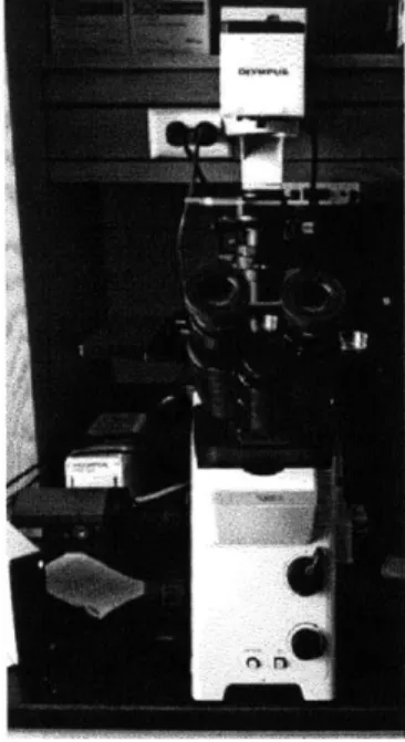
Figure 6.4: Olympus Microscope ... 59
Figure 6.5: Microscopy Images of Oxygenated Fluid ... 60
Figure 6.6: Blood Gas Machine ... 60
Figure A.1: Motor Speed vs. Force curve ... 67
Figure B.1: Budget... ...68
Figure C.1: LabView - Open Motor Channel ... 60
Figure C.2: LabView - Open Limit Switch & Load Cell Channel...70
Figure C.3: LabView - Close Channels ... 71
Figure C.4: LabView - Initialize Phase... 72
Figure C.5: LabView - Bellows Top Phase... 73
Figure C.6: LabView - Manual Jog Phase... 74
Figure C.7: LabView - Calibration Phase (1 of 2)... 75
Figure C.8: LabView - Calibration Phase (2 of 2)... 76
Figure C.9: LabView - Motor Control Phase (1 of 3)... 77
Figure C.10: LabView - Motor Control Phase (2 of 3)... 78
Figure C11: LabView - Motor Control Phase (3 of 3)...79
Figure C.12: LabView - Math Sub-VI...80
Figure C.13: LabView - Error Sub-VI (1 of 2)... 81
TABLES
Table 2.1: Functional Requirements...16
Table 3.1: Fluid Analysis ... 22
Table 3.2: Resistance Calculations...24
Table 3.3: Revised Fluid Analysis ... 25
Table 3.4: List of Plumbing Components and Connections ... 28
Table 6.1: Theoretical Mixing Proportions...55
Table 6.2: Experimentally Observed Mixing Proportions ... 56
Table 6.3: Mean Particle Diameters ... ... 58
CHAPTER
1
INTRODUCTION
1.1 PURPOSE
The purpose of this project is to explore in detail the design and optimization of a pump to deliver a specified volumetric flow rate of an oxygenated fluid. Dr. John Kheir works at children's hospital and has developed a fluid that can re-oxygenate blood in non-breathing patients. The fluid is compressible and presents many problems when being pumped using conventional medical devices such as peristaltic or syringe pumps. The main problem with these pumps is that since the fluid is compressible, the set infusion rate does not necessarily indicate how much fluid is dispensed.
This thesis will investigate how a pump was developed, including the analysis performed to correctly choose and size different components such as motors and sensors. It will detail how the pump was designed to be modular, low cost, and have the potential to save life.
1.2 MOTIVATION
In medical emergencies, an oxygen-starved brain quickly suffers irreparable damage. In many cases, patients who stop breathing can be resuscitated but suffer from brain damage. The
objective is to build a device to infuse a specialized suspension which oxygenates the bloodstream, allowing for more time to resuscitate a patient before they suffer brain and/or organ damage. The oxygenated fluid and delivery system could improve medical outcomes for patients with cardiac arrest, which currently has a neurologically intact survival rate of sub-five percent.
Oxygen is required to maintain cell homeostasis in the human body. Serious organ injury and death can occur in critically ill patients experiencing asphyxia, lung injury, and cardiac arrest because they cannot consume the amount of oxygen needed to survive. This oxygenated fluid raises oxyhemoglobin saturation upon injection, and can improve the survival rates of critically ill patients [1]. Because current medical infusion pumps make the assumption that the amount that the plunger depresses is directly proportional to the volume injected, the injected volume does not to be measured. However, when a fluid is compressible, the amount dispensed by the plunger being depressed is not proportional to the volume injected. Therefore, the amount of oxygen a patient receives from the oxygenated fluid is not known. The device outlined in this thesis will account for this discrepancy.
1.3 PUMP OVERVIEW
The pump design can be broken up into three modules: the oxygenated fluid dispenser, the saline dispenser, and the mixer. The oxygenated fluid dispenser consists of the bellows, a linear actuator to compress the bellows, and a feedback control system. The saline dispenser consists of a peristaltic pump. A plate attached to linear actuator will compress the bellows. Between the plate and the bellows top is a load cell that will provide the data for the feedback control. Both the oxygenated fluid dispenser and the saline dispenser have tubing that guides the respective
fluids to a wye junction where they meet and are then mixed by a static helical mixer. The system diagram is show bellow in Figure (1.1).
Figure (1.1) - This figure shows the overall system diagram.
The flow also passes through a bubble trap before the fluid can be injected into a patient. More detail about each of the major components, how they were selected and their functions is outlined in Chapter 3.
1.4 PRIOR ART
Research was done to find previous pumps that were used for other unconventional fluids. From exploring these different options, a few ideas were incorporated into the design for the oxygenated fluid pump described in this paper.
1.4.1 Belmont Rapid Infuser
The Belmont Rapid Infuser is a high efficiency electric warmer coupled with a high-speed peristaltic pump [2]. It is capable of measuring flow rate, the temperature at the inflow and outflow of the heater, patient temperature, and line pressure. It can also detect and trap air bubbles before infusion into the patient. This device however uses a peristaltic pump, which is not sufficient for the oxygen suspension because the pump causes cavitation in the fluid. It is also not capable of compensating for fluid compression when calculating flow rate. Though the full system cannot be used, the bubble trap was extracted for use in our design because it should be capable of handling high flow rates.
1.4.2 Enhanced ACL Repair Gun
The enhanced ACL repair gun is the product of a previous 2.75 project that allows for proper mixing and heating of a fluid [3]. The gun has a heating unit on one end of gun and an adjustable auger that mixes fluid when deployed; this product faced the mixing challenge that also needs to be addressed in the dilution of the oxygenated fluid. The auger inspired the use of passive mixing techniques involving helical structures for this device.
CHAPTER
2
FUNCTIONAL REQUIREMENTS
2.1 DESIGN REQUIREMENTS
The primary goal of this design was to deliver IL of the oxygenated fluid at a specified volumetric flow rate. From this and in discussion with Dr. Kheir the following functional requirements and accompanying parameters were identified:
Table (2.1) - The functional requirements of the Oxygenated Fluid Pump.
Flow rate accurate to 10%
(must dliverfluid between 10 and 200mL/min into 14 gauge catheter)
Can handle at least IL fluid
Mix with saline,
Will not degrade fluid
Maintains sterility, Portable (nice to have) Maintainable or disposable
Cost appropriate Traps bubbles'
Flow sensors; valves controller
("the-set infusion rate on thepump does not indicate what is delivered")
Reservoir system Static or kinetic mixers Limits on pressure
(upper limit: 10psi)
Limit contact withiluid -. Minimize size, mass
Cheap plastic parts,
The functional requirements in Table 2.1 were the minimum requirements that had to be met to complete the task Dr. Kheir gave to us and to ensure we had a reliable pump. They are outlined in this chapter with more detail, including how some of the decisions for the design parameters were made.
2.1.1
Cost
Medical devices are extremely expensive. Standard syringe pumps and peristaltic pumps cost anywhere from $500-$4000. The goal for the oxygenated fluid pump described in this project was to keep it around this same price range. A table of all the components purchased and the total cost can be found in Appendix (B).
2.1.2 Flow Rate
The flow rate for our pump is relatively high, set by Dr. Kheir. He determined that it would take about IL of the oxygenated fluid for a human to survive around 5 minutes. Therefore, the flow rate was established to be 1L in 5 minutes or 200mL/min or around 3.3mL/s with an accuracy of ±10%. This is how much fluid needed to be pumped into the patient at a 70% concentration. There are separate flow rates however for the peristaltic pump and the bellows pump. Since the fluid started at a concentration of 90% and needed to be mixed to 70%, it was determined that a mixing of about 250mL Saline and 750mL of the 90% concentrated oxygenated fluid was necessary. Therefore, the flow rate for the peristaltic pump was set at 250mL in 5 minutes or 50mL/min or about 0.83mL/s. The flow rate for the bellows pump was determined to be 750mL in 5 minutes or 150mL/min or 2.5mL/s.
2.1.3
Mixing
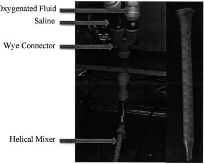
As mentioned before the oxygenated fluid needs to be mixed from a 90% concentration to a 70% concentration. A static mixer was chosen instead of a kinetic mixer because a kinetic mixer could potentially damage the bubbles. Also, it wasn't too difficult to mix the oxygenated fluid with saline and a static helical mixer was determined to be enough. To mix the fluid with saline there were two different paths that met at a wye junction and then into the helical mixer.
Oxygenated Fluid Saline
Wye Connector
Helical Mixer
Figure (2.1) - Layout of fluid path into the helical mixer and close up view of mixer.
The helical mixer used was from an epoxy gun. From running some basic tests it was determined that this mixer did an adequate job at mixing the fluid. More information of mixing and determining the quality of the fluid after mixing can be found in section 6.1
2.1.4 Capacity
Dr. John Kheir determined that an appropriate amount of fluid to be pumped into a human in order to ensure proper oxygenation was 1L. Syringes that hold IL of fluid are hardly found in the medical field and the frictional forces found in a syringe are hard to deal with. Taking into account that this had to be a large compressible container, a bellows was found to be appropriate. Bellows have predictable forces that can be easily modeled as a spring and are found in a variety of sizes. More information on bellows and volume can be found in section 3.2.4.
2.1.5
Medical-Specific Requirements
Not degrading the fluid, maintaining sterility, trapping bubbles and the accuracy of the flow rate are all medical-specific requirements. It is extremely important that during the pumping process, no more than 10 psi is exerted on the fluid in order to ensure the fluid is not damaged. This requirement was also given to us by Dr. John Kheir. It is important to maintain sterility throughout the pumping process. Therefore, the pump was design so that the major components are replaceable. For example, the mixer is cheap and replaceable, the bellows pump functions as a cartridge in which you can just replace the bellows with another one once empty, and the saline pump only requires the saline bag to be changed. Trapping the bubbles is an extremely important part of the design because if there are large bubbles flowing into the patient it can cause an embolism. Last but not least the accuracy of the flow rate is extremely important requirement because the exact amount of fluid being pumped into a patient needs to be known. The whole pump is designed to fulfill this functional requirement first and foremost.
CHAPTER
3
MODELING
3.1 SYSTEM FLUID MODEL
Sizing of different components in designing the Oxygenated Fluid Pump required correctly modeling the fluid as it moved through the pump. Because of the fluid viscosity, it is important to size the components correctly to achieve the desired flow rate. The modeling done in this section helped size the bellows and select the motor and load cell.
3.1.1
Pressure
Basic pressure analysis was done using the Hagen-Poiseuille equation:
_8piLQ
AP = 4 (3.1)
rr4
where:
AP is the pressure drop L is the length of the pipe
Q
is the volumetric flow rate r is the radius of the pipe p is the viscosity of the fluidThis equation is for finding the pressure drop in a pipe where the length is much longer than the diameter of tie pipe, which is true in this case. However, this equation also assumes that the flow is laminar, viscous and incompressible. The fluid being pumped in this case will meet all of these
assumptions except that it is compressible. This analysis is still valid however because its purpose is to make a first order approximation that will allow for the correct sizing of components.
Standard tubing was used, along with luer locks (medical grade connectors) to make the initial layout of our device shown in Figure (3.1).
Bellows B Saline Bag A Saline Pump Mixer C
Figure (3.1) - This figure shows the basic layout of the pump in order to fulfill the functional
requirements.
Sections A, B and C represent the different sections of tubing that fluid flows through. Using this
general layout and the Poiseuille equation (3.1), other dimensions were approximated (such as
radii and lengths of tubing) and analysis was done to approximate the resistance from each
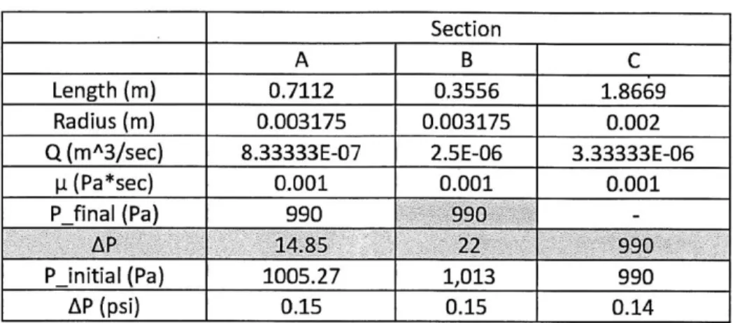
Table (3.1) - This table shows the analysis done using Poiseuille's equation.
Section
A B C
Length (m) 0.7112 0.3556 1.8669
Radius (m) 0.003175 0.003175 0.002
Q (m^3/sec) 8.33333E-07 2.5E-06 3.33333E-06
pi (Pa*sec) 0.001 0.001 0.001
P final (Pa) 990 990
-AP 14.85 22 990
P_initial (Pa) 1005.27 1,013 990
AP (psi) 0.15 0.15 0.14
The pressures calculated are gauge pressures. The flow rates in each section come from the functional requirements of the pump. Because fluid needs to be mixed from 90% gas by volume to 70% gas by volume and the desired flow rate is IL in 5 minutes, it was possible to calculate the desired flow rates for sections A,B and C. By mixing 150mL/min (in section B) of the oxygenated fluid at a 90% gas by volume concentration with 50mL/min (in section A) of saline, the final concentration would be at 70% gas by volume at a flow rate of 200mL/min (in section C). These flow rates were then converted to SI units and were used in the calculations in Table (3.1). From this analysis we were able to get a basic idea of the pressure drops in each section, however, this initial analysis was determined with the viscosity of water, which is much lower than the oxygenated fluid viscosity. Therefore, the resistances for each section were calculated in order to proceed with the analysis.
3.1.2 Resistances
By calculating the resistances from each section of tubing it was possible to refine the model above to more accurately reflect the pressure drops and eventually how much force is needed to
achieve the desired flow rate. Resistances were calculated by simplifying the Hagen-Poiseuille equation. If
AP = RQ (3.2)
then the resistance is,
8 pL R = i-;
s7r
Before calculating the resistances, it was important to select the correct viscosities for each section. In section A, the viscosity of the fluid saline was used (which was approximated to be the about the same as water) but for sections B and C, it was necessary to find the viscosity of the fluid at a concentration of both 90% and 70%. The viscosity of the fluid at different concentrations was found by using a rheometer and the data provided by doctor John Kheir is shown in Figure (3.2).
d
Shear Stress Sweep101
0
0
Cn
0.1 1 10
Stress (a, Pa)
+90 vol %
+80 vol % + 65 vol %
-Blood
100 1000
Figure (3.2) - Viscosity of oxygenated fluid at different concentrations found using a rheometer.
Using the chart in Figure (3.2), the viscosity of the oxygenated fluid at a 90% concentration was approximated to be around 10 Pa*s and at 70% concentration it was approximated to be around 0.1 Pa*s. Imputing these new viscosities into the model and using equation (3.3), the following resistances were calculated shown in Table (3.2)
Table (3.2) - Resistances calculated for each section using equation (3.3) and the viscosities estimated from figure (3.2).
Section. A B C
Ressance 17,822,021 89,110,103,498
29,712,636,326
With the resistances calculated above, it is possible to calculate how much force will be needed to achieve the flow rate necessary if the area of the top of the bellows is known. The bellows selected hold slightly more than IL of fluid. It has a diameter at the top of 115mm, a height of 150mm, and an inner cylinder of diameter 90mm (for more information on bellows selection and calculation refer to section 3.2.4). Using the equation,
F = PxA (3.4)
The force needed to compress the bellows and achieve the flow rate desired was about 700 lbs or around 3300 N. A motor that could achieve this force and still have the resolution and control needed for this application was not readily available. Therefore, the model was changed in order to decrease the resistances in each section. By examining Poiseuille's equation, it was determined that the best way to decrease the resistance would be to increase the radius of the tubes in each section. Since, the viscosities and flow rates are fixed, the only other parameters that could be changed are length and radii of each section. However, decreasing the length of each section is not as affective as changing the radii because the radius is a quadratic term. By
changing the radii and decreasing the lengths of different tubing sections it was possible to decrease the force needed to achieve the desired flow rate to around 60 lbs or about 250 Newtons. The new parameters and calculations are shown in Table (3.3).
Table (3.3) - Revised analysis performed using Poiseuille's equation. Section
A B C
Length (m) 0.6604 0.1397 0.8669
Radius (m) 0.003175 0.0047625 0.003175
Q (m^3/sec) 8.33333E-07 2.5E-06 3.33333E-06
i (Pa*sec) 0.001 10 0.1
P final (Pa) 7,V241 7,F241
AP 13.79 17,288 7,241
P initial (Pa) 7255.04 24,529 7,241
AP (psi) 1.05 3.56 1.05
Force (N) N/A 255 N/A
Force (Ibs) N/A 57 N/A
Resistance 16,549,019 6,915,069,760 2,172,372,011
By comparing tables (3.1) and (3.3) it is shown that changing the radii and lengths of tubing significantly reduced the resistance in sections B and C. With a force of 60 pounds, the design process can now proceed and the appropriate motor and load cell can be selected.
3.2 PUMP DESIGN
The pump design described in this section was carefully constructed to meet all of the functional requirements mentioned in Chapter 2. The basic structure of the pump was designed based on the fluid modeling in section 3.1. This section will use that fluid model to describe some of the decisions made in selecting the components. It will also go into detail and analysis of different components of the pump design and the reasons behind the choices made.
3.2.1
Structure
The frame and structure of the pump was built using 80-20 structural elements. The 80-20 was selected because it would allow for a very modular design that can be easily assembled. Since the bellows had a diameter of about 120mm or about 4.7 inches, the frame was designed to be 8 inches wide so that there was about 2 inches on either side of the bellows. It was important to have a reasonable gap on either side of the bellows to facilitate loading. The top of the structure has an 8 by 8 plate " thick in which the electronics and motor are mounted to. The motor is mounted in such a way that the lead screw is attached to a plate that is guided by the rails on the 20 and push down on top of the bellows. The bellows sit on a plate, which is fixed to the 80-20 rails slightly above the center of the structure. There is also another structure off to the side of the main structure in which the peristaltic pump sits on. The basic structure of the pump is shown
in figure (3.3). 1
3.2.2
Tubing and Connections
Most of the tube sizing was determined in the fluid model in section 3.1. The lengths used in the model were adjusted so that all of the components were connected. The tubes were connected using different push to connect junctions. The tube connected to the bellows pump meets the tube connected to the peristaltic pump at a wye junction. The tubes then go on to connect to the static helical mixer and to the bubble trap. All the components are shown in Figure (3.4) and listed on table (3.4).
Figure (3.4) - All the plumbing components and connectors
The plumbing components are labeled in Figure (3.4) above with numbers 1-8 and are listed in Table (3.4) below:
Table (3.4) - Outlines all the plumbing components and their dimensions shown in Figure(3.4).
2 Ball Valve M2" NPTF to 2" MIP
3 Pipe Thread to Quick Connect M"MIP to M" 'Tube
4 Tubing 'A" Tube
Wye Quick Connect '" Tube
6 Quick Connect Reducer '2" Tube to 3/8" Tube
7 Helical Mixer N/A
8 Bubble Trap N/A
3.2.3
Motor & Load Cell Selection
Both the motor and the load cell were selected based on the force calculation determined from
the fluid model. The force needed to achieve the desired flow rate of 200mL/min as specified by
doctor John Kheir is about 60lbs. The motor selected for this application was a stepper motor that can operate at a maximum force of 100 lbs and has a step size of 0.001". The force vs. linear
velocity curve for the motor can be found on appendix
0.
The load cell selected was an OmegaLCFD-100 that can sense forces up to 100 lbs also. It is attached to an amplifier, which outputs a
signal large enough to be read by the LabView DAQ board.
3.2.4 Bellows
Bellows are a good choice for this application because of the different functional requirements it
easily measured and modeled as a spring. Commonly, syringes are used for medical pumps however syringes are rarely found with a IL capacity and the friction force generated by the seal in the syringe is complex to model. The bellows is also a good choice because of the volume compression method that is being used. As mentioned before, the bellows has a diameter of about 120 mm, a height of about 140 mm, and an inner cylinder of diameter 100 mm.
Some slight modifications had to be added to the bellows. On the top of the bellows, a small luer lock is attached and acts as a purge valve. Once the bellows is full of fluid, the top can open so that the excess air can be purged out of the bellows. Also, the bottom of the bellows is open and threaded, therefore, a 3-D printed cap was made in order to close the bellows and create a container. The cap was specifically designed to create a seal between the bellows and the cap. Adding a cap also made it easier to load up the bellows with the oxygenated fluid. Figure (3.5) below shows the bellows with the cap and purge valve.
3.2.5 Bellows Cap
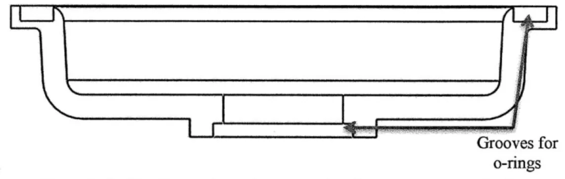
A cap was designed for the bellows in order to make it a closed container. It was designed so that it would thread into the bottom of the bellows and create a perfect seal. To create the proper seals, o-rings were incorporated into the design. Figure (3.6) shows the cap design,
Grooves for o-rings Figure (3.6) - This figure shows the cap design with grooves for the O-rings.
In designing the grooves for the o-rings it was important to dimension the part correctly so that
the ring has space to deform. Figure (3.7) more closely shows what is happening.
O-ring
Diameter = D
0.9D
1.1ID
Figure (3.7) - This is the geometry necessary to create a seal.
In figure (3.7), it is show that the height of the groove has to be 90% of the o-ring diameter and
compressed, it will deform and push against the side of the groove, creating a perfect seal. This technique was used in two places to create a seal between the bellows and the cap, and to create a
seal between the cap and the straight-thread to NPT connector.
The finals design of the bellows cap is shown bellow in Figure (3.8). The image on the left is the CAD model from solidworks designed by Alex Mason to thread into the bottom of the bellows. The image on the right is the actual bellows cap after it was 3-D printed. The initial cap was created using a 3D printer provided by MIT's Center for Bits and Atoms, and 3D Printsmith LLC printed a second version. Large-scale production would use injection molding.
Figure (3.8) - 3D CAD model of the cap on the left along with the actual 3D printed part on the right.
3.2.6
Volume Calculation
Calculating the exact volume of the bellows was a really important step in calculating how that volume changes as it is being compressed. The total volume of the bellows was determined to be 1.28 liters. This volume is more than the specified IL because when the bellows is fully compressed, there is still some fluid inside it. This is because the bellows can compress a maximum of about 83mm. This means that when the bellows is fully compressed, it is still
volume of about 1005mL, which is right around what is needed to dispense due to our functional requirement. In reality, the bellows needs to displace only around 750mL of fluid because the functional requirement states that 1L of the fluid needs to be dispensed but that is at the 70% concentration. Since the bellows is holding the 90% concentrated fluid, it still has to be mixed with saline, which is where the other 250mL comes in.
After measuring how much fluid the bellows can hold, the volume displaced as the bellows is being compressed was calculated. This calculation took several steps. The first step was calculating the volume displaced as the inner cylinder of the bellows got smaller. Figure (3.9) demonstrated this section.
Figure (3.9) - The shaded blue portion indicates the inner cylinder of the bellows.
Calculating the volume of the shaded portion in Figure (11) was done by using Equation (3.5) below:
V, =x r2L (3.5)
where r is the radius and L is the displacement of the bellows. The radius of the center cylinder section was measured to be 50mm. The length of the bellows was measured to be about 130mm giving the center section a volume of approximately 1.02 liters. To model the volume displaced as the bellows is being compressed, L was turned into a variable. The next step was to calculate
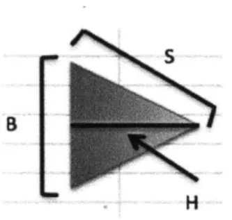
the volume of the un-shaded portion of Figure (3.9). This part was much more complicated. The ridges were modeled as triangles as shown in Figure (3.10):
H
Figure (3.10) - Triangle used to model the cross section of the ridges of the bellows.
In Figure (3.10), B is the base of the triangle, H is the height and S is the side. As the bellows is being compressed, the base of the triangle changes. Since the side (S) is a constant dimension of the bellow, then the height of the triangle also changes as the bellows is being compressed. To simplify calculations, only half of the triangle was used and then was multiplied by two. Using this cross sectional area, the shell method show in equation (3.6) was used to calculate the volume of the ridges.
ridges = 2xfr{ f {x)dx (3.6)
f(x) is the equation determined by the line with a slope of S. The limits of integration were determined by the radius of the bellows from the center until the outside of the bellows or as the radius goes from r to r + H. f(x) was determined by equation (3.7) below:
f(x)=- x+Y (3.7)
2H)
where Y is the y-intercept. For example, Figure (3.11) bellow shows an example of the graph created when B is 5.9mm, H is 12.5mm and Y is 28.32mm. Y was determined by using the linear
equation y = mx + b and the x-intercept of 60 because that is the maximum radius and that is achieved when B/2 is zero.
-20
S
Figure (3.11) -An example of the cross-sectional area that was used to find the volume of the ridges on the bellows.
H was found by using the equation of a circle with S being the radius and the center of the circle
set at x = 60 and y = 0. This is shown in Figure (3.12) below:
Most Compressed Position B B I S H N i / / / Most Expanded Position
Figure (3.12) - Demonstrates how H changes as B is getting smaller, representing the bellows being compressed.
By repeating this method as B decreases to zero and as H approaches S, then multiplying to account for all the ridges, the volume displaced by the ridges turned out to be around 240mL.
Adding this to the volume displaced by the center cylinder the total volume displaced was calculated to by about 1.26L, which is extremely close to the measured volume of 1.28L. This approximation can get closer by measuring the dimensions of the bellows with more precision however because the flow rate needs to be accurate to ±10%, this approximation is sufficient.
3.2.7
Sliding Mechanism
The sliding mechanism is the most important mechanical component of the pump. It is what aligns the lead screw of the motor and allows the bellows to be compressed in a vertical motion with the force being straight down on top of the bellows. The sliding mechanism consists of a few components shown in Figure (3.13).
Figure (3.13) - Sliding mechanism and its corresponding components.
The geometry of the sliding mechanism was the most important part of its design. The distance from the top of the upper sliding bracket to the bottom of the lower sliding bracket has to be at least 1.6 times the distance from the left rail to the linear screw. This needs to be true because it
characteristic length and L in this case is the length of the sliding brackets. D was measured to be around 94 mm and L was determined to be about 150 mm in order to fulfill St. Venant's principle. If up and down makes up the y-axis, left and right make up the x-axis and in and out of the page the z-axis, then the sliding brackets prevent motion in the positive and negative x and z directions as well as rotation around the z and x axes or 4 degrees of freedom. The outrigger on the other side prevents rotation around the y- axis. The only degree of freedom left is travel in the y direction, which is the intended direction of travel. This mechanism relies on the guiding rails on either side to be as parallel as possible or else jamming would occur. The sliding mechanism designed here works well and was an easy, reliable way to compress the bellows.
3.2.8
Peristaltic
Pump
Saline is pumped by a Fisher Scientific Variable-flow peristaltic pump, which is controlled manually. The peristaltic pump is capable of producing flow rates from 30mL/min to 100mL/min, which covers the required range. The pump is a simple device that is familiar to doctors and nurses. We decided to use a peristaltic pump because of its ease of use and its minimal contact with the fluid. One problem encountered however was that the peristaltic pump used was not reliable. With a saline bag standing upright, the flow would vary greatly on the same setting because of the difference in pressure as the level of saline drops. Therefore, the saline bag was laid on its side and the pump functioned more reliably. Ideally, a better peristaltic pump would be purchased.
The final module of the design is the mixer, which combines the oxygenated fluid with saline. This reduces the concentration from 90% to 70% gas by volume, which in turn reduces the viscosity of the fluid and makes it suitable for infusion. The concentrated oxygenated fluid and saline meet at a wye-junction to minimize damage to the fluid. They then combine and pass through a single plumbing path into a static, helical mixer, similar to an epoxy mixer.
CHAPTER
4
PUMP LOGIC
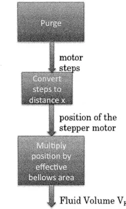
The novelty of the oxygenated fluid pump is in the control system. It is broken down into three main phases: a purge phase, a calibration phase and a motor control phase. The logic of the pump is displayed in the diagrams below:
motor
stei s
position of the stepper motor
Fluid Volume VFO
Figure (4.1) - Pump logic diagram: Purge Phase
The purge phase is utilized to purge the bellows of all unwanted air. It is assumed that while loading the bellows with fluid, some air will be trapped. This first step will get rid of the air and calculate a new volume which is set as the initial volume of fluid in the bellows. The next step is calibration, which is displayed below:
Figure (4.2) - Pump logic diagram: Calibration Phase
The calibration phase is necessary because the fluid properties are not consistent every time. Also, the bellows may not be filled the same every time or some of the fluid may have degraded faster than others. The calibration will first ensure that the fluid properties are within reasonable range then determine the compressibility constant for that particular batch before starting to pump. Right now, the calibration phase is being used to help characterize the fluid. The motor control phase is completely dependent on this calibration. Ideally, once the fluid is characterized there will be a model used for an ideal fluid in which case the calibration won't be necessary anymore. If anything it will be used to categorize the fluid as ideal or non-ideal. If the fluid is non-ideal then another batch will have to be used.
The calibration phase works by taking the initial fluid volume and calculating 90% of that
volume. Then the number of steps the motor needs to travel is calculated. The motor goes to this
set position and records the force on the load cell at every step and makes a graph. This graph is basically the spring force the fluid exerts as it is being compressed.
Send initial Desired motor speed + error
New motor speed
Uncompressed volume VF(N+1)
Proportional
motor speed error
Figure (4.3) - Pump logic diagram: Motor Control Phase
The motor control phase is the most important phase in the control system and the most complicated. As the motor is moving down, the force is being measured. This force is then used and compared to a force that matches it closest in the calibration graph. Then, a corresponding volume is calculated using this reading, which is then used to calculate a flow rate. This flow rate is compared to the desired flow rate (set by the user) and an error is calculated. This calculated error is then converted into an error in velocity. The error in velocity is finally added to the
current velocity of the motor, which will speed up or slow down depending if the error is positive or negative. The load cell then reads another force and the process is repeated. This phase is better outlined in the Labview section 4.2.5, where the controls are explained in detail.
4.2 LABVIIEW
The code was written in Labview using a phidgets controller and a DAQ board. A phidgets library was downloaded from the phidgets website. The software progresses through a number of stages; in order, they are "Initialize", "Bellows Top", "Manual Jog", "Calibration", and "Motor Control", and "End".
- "Initialize" checks connections and makes sure the stepper motor is ready to be operated.
e In "Bellows Top", the stepper motor moves downward until a non-zero force is detected.
This indicates the top of the bellows.
* "Manual Jog" allows the user to manually control the position so that all the air from the bellows is purged before calibration.
e The "Calibration" stage performs a test compression of the fluid and determines its
compressibility curve, as this may vary from batch to batch.
e The "Motor Control" stage dispenses fluid with a force feedback system. e "End" cleans up the program and closes the operation of the stepper motor.
The next few sections will outline each of the six steps outlined above in more detail. The six stages above are inside a case structure. A case structure has one or more sub-diagrams that execute once the structure executes. This case structure is inside a while loop, which repeats the sub-diagram inside it until another value indicates it to stop. In this case, a stop button will stop
the loop. Outside the while loop are channels that only need to be open once. For example, it opens up the channel to communicate with the motor through a phidgets controller. It also opens up the limit switches and the load cell reading. Once these channels are open, they can be utilized at any point in the rest of the code. The only other component outside of the while loop is the close function, which closes communication to the components that were opened. The rest of this chapter will go on to explain each of the six cases inside the case structure.
4.2.1 Initialize
The purpose of this stage is to raise the bellows plate to it highest position to allow for easy loading of the bellows. The first block sets the velocity limit of the motor to any set constant value. The second block set the target position. The way this works is that a shift registry is used. The first thing that needs to be known is that this case is going to be repeated inside the while loop until it is told to move on to the next case. The shift registry remembers the last set input of a block and carries it back around the while loop. Using this knowledge, one step is added to the motor position every time the loop runs. For example, when the case executes for the first time, the default target position is one, then the shift registry remembers that value. The second time the case is executed, the shift registry remembers the value of one and adds one to it to make it a value of two. This value is then set as the new target position. This way, the motor will continue to increase step by step until it is told to stop.
There is only one caveat; the code should not run faster than the speed of the motor. The velocity limit has to be the limiting factor in how fast the motor moves. The reason for this is that if the code is running faster then the motor speed, when the command to stop is executed, the motor will not be at the set target position and will continue to move until that position is reached. If the
motor velocity is the limiting factor though, as soon as the stop command is executed, the motor will stop moving.
A limit switch in this case activates the stop command. As long as the limit switch reads a negative value, the motor will continue moving the bellows plate up. Once the limit switch is pressed, the motor will reverse its direction and move until the limit switch is un-pressed. This is done by using a true/false case structure. A comparison block is used to compare the value of the limit switch to a "true" Boolean value. Once the value of the limit switch is true, or when it is pressed, the code will execute the sub-diagram inside the true/false case structure. When the case is false, nothing happens. When it is true, a new target position is set which will move the motor plate down until it the limit switch is no longer active. The true case structure also tells the code to move to the next case, which is the Bellows Top case. Last but not least, there is a wait function inside the true/false case structure that waits until the motor gets to the un-pressed limit
switch position.
4.2.2 Bellows Top
The purpose of this stage is to find the top of the bellows. Much in the same way the initialize state works, a value of one is added to the target position using a shift registry until it is told to stop. The only difference is that the motor is moving the bellows plate down instead of up. The stop command in this case is also different. Instead of a limit switch activating the comparison block it is the limit switch value. The comparison block is once again connected to a true/false case structure. If the load cell reads a value greater than a specified value greater than zero, it executes the sub-diagram inside the true case of the true/false case structure. Once again, the false case is just empty, allowing the motor to continue moving down. When the comparison
block reads a true value however, the true case is activated. The true case simply tells the motor to stop and moves the code to the Manual Jog case. Therefore, the Bellows Top case moves the motor until the load cell reads a value greater than zero, in which case it stops and the top of the bellows is found.
4.2.3 Manual Jog
The goal of the Manual Jog case is to allow the user to manually control the position of bellows top. In this state, the purge valve will be opened, then the user can manually slide a control and compress the bellows until all of the air is purged from the bellows. At which case the purge valve is closed and calibration can occur. The first step in this case is to set the current position to zero. This needs to be done because once the bellows is purged, this position sets the initial fluid volume that will be used in other calculations down the road, including the error calculation. This position is set to zero by using yet another true/false case structure. This case structure is set to a default false value. A true/false switch, also set to a default false value, activates it. Once the case is executed once, the position is set to zero and the value on the true/false switch changes to true. The true case of the case structure is just empty, allowing the code to continue.
The next step in the code is an event structure. An event structure has one or more sub-diagrams or event cases, one of which executes once the structure executes. The default event just gets the motor position. It does not actually move the motor, it just tells the user where it is from the zero position. The second event in the event structure is just a block with the target position, which is controlled by a slider. When the slider moves, it tells the motor to go to that position. When the manual jog is complete, a button tells it to go to the next case, which is the Calibration case.
When the button is not pressed, the Manual Jog state just keeps running. Once the button is pressed, the calibration state is initiated.
4.2.4 Calibration
The calibration state is one of the most important states. The goal of the calibration state is to compress the bellows and get a calibration curve or a compressibility curve for the fluid. It does this by first finding the position of the bellows. Then it takes the manual jog position, calculates how many steps need to be taken in order to compress the bellows to 90% of its volume after the
manual purge. It does this math using a sub-VI or sub virtual interface described in detail in Appendix (C).
The number calculated is then entered as the number of iteration for a for loop. A for loop executes its sub-diagram n times where n is value entered by the user, in this case, the number of steps needed to compress the bellows to 90% of its volume. 90% was chosen because
compressing the bellow to 90% of its original volume generates a force large enough to set a limit on the force. During execution of the motor control, the force should never go above the force needed to compress the bellows to 90% of its volume.
Once the number of iterations is set, a shift registry takes the iteration that it is in, then adds that number to its position after the manual jog. Therefore, if the motor is in position 50 after the manual jog and the for loop is in its first iteration, then the motor is set to a target position of 51. During the second iteration the target position is set to 52 and so on. These positions are also being recorded into an array, along with a force reading at every step. Last but not least, inside
the for loop, the program is set to record force values only if they are larger then its previous value, making it monotonic.
Once the for loop is complete, the values are inserted into a sub-vi that calculates a %volume. This percent volume is basically what volume the compressible fluid will expand to at atmospheric pressure. This calculation is also explained in Appendix (). After the %volume is calculated, a graph of %Volume vs. Force, which is referred back to in the motor control stage is created. Last but not least, the motor is set back to its starting position, after the manual purge. Another button tells the code to proceed into the motor control state.
4.2.5 Motor Control
The motor control phase use a force feedback system in order to control the motor. The first step it does is set a target position to the bottom of the stroke of the bellows. A position that will guarantee the bellows becomes fully compressed. The motor control state functions around a sub-vi, which calculates the motor speed error. This sub-vi has six inputs.
One of the inputs is found when the load cell reads a force. This force is rounded to the nearest integer. The force vs. % volume graph from the calibration state is also rounded to the nearest integer. The code then compares the force read to the array from the calibration state and finds a value that matches the force exactly. Once this force is found, the index is recorded and the corresponding %volume is displayed. This value is then inserted into the sub-vi that calculates the error. If the force is not matched exactly, a shift registry makes sure that the previously matched force is inserted instead.
Another input is the amount of steps a motor moves in one loop. This is found by getting the current position at the beginning of every loop, and using a shift registry to subtract the previous position recorded. This change in position is also used to calculate another input. The current velocity of the motor is read and the number of steps moved in each loop is divided by this current velocity in order to calculate a time step for each loop. The last three inputs are the desired flow rate, the uncompressed volume calculated at a previous step (initial value is 0, later values are determined by using a shift registry) and the manual jog position.
These inputs are used in the following order to calculate an error in motor speed. The manual purge is used along with the number of steps traveled in each loop are used to calculate a volume of fluid displaced. That number is then divided by the %Volume input in order to find the volume at atmospheric pressure. This volume is then subtracted by the previously calculated uncompressed volume (in the first iteration it is zero). This volume is then divided by the time input in order to find a flow rate. This flow rate is then compared to the desired flow rate input
and an error is calculated. This error is the divided by an effective area of the bellows in order to get an error in velocity.
A small constant multiplies this error in order to create a proportional control. If the error is negative, it will slow the motor down, if it is positive then it will speed the motor up. An extra
measure of safety is also added. The previous velocity measured is multiplied by 120%. If the new velocity calculated after the error was added to it is greater than 120% of the old velocity, a new velocity is not set. This will ensure that the pump does not increase its speed too quickly.
The motor control is only stopped when a limit switch is pressed. It works in the same manner as the previous limit switch in the initiate case, by using a true/false case structure. Once the
true/false case structure achieves a true value, the motor position is set back up to un-compress the bellows and the code moves on to the final end state.
4.2.6 End
The end state is just a blank sub-diagram that waits for the motor to move back up until the bellows is uncompressed. Once the motor reaches its target position, the code will just continue running a black diagram until the stop button is pressed, in which case communication to the motor, limit switches and load cell are closed and the code stops running.
CHAPTER
5
EXPERIMENTATION
5.1 FLOW RATE
The flow rate for both the peristaltic pump and the bellows pump needed to be determined experimentally. It is essential that the pump functions properly and delivers the flow rate with a
10% maximum error. Some experiments are described below, showing the reliability of the flow rates of each of the pumps.
5.1.1
Peristaltic
Pump
For the first test, the flow rate of the peristaltic pump will be measured. This test will ensure that the pump is reliable and will pump out a consistent amount of saline every time. Three minutes was chosen as the test time because the pump will be pumping for a total of 5 minutes at a time (5 minutes is the time we will deliver 1 L of mixed fluid) and figured that if it pumps steady for 3 minutes then it will be fine with 5. The main concern is that the pump needs to be consistent in order to deliver well-mixed fluid. The flow rate has to be the same -whether the bag is full or half full.
0 20 40 60 80 100 120 140 160 180
Time (s)
Figure (5.1) - This figure shows the flow rates measured for the peristaltic pump on 5 different
trials
These test resulted in an average flow rate of 84.9 ± 10 mUmin, which is not accurate enough for our system. The flow is linearly increasing; however, there is too much deviation between each trial considering the input setting/speed of the pump was the same. It turns out that as the volume in the saline bag changed, the flow rate changed. As stated in the functional requirements, the flow rate needs to be accurate to ± 10% and has to be consistent whether the bag is full or not. A different experimental setup was then attempted in which the saline bag was horizontal with an aluminum plate on top of it. An average flow rate of 85.5 mUmin was found with a standard deviation of 2.4 mUmin. This test ensured that the pump is reliable and will
pump out a consistent amount of saline in every use if the saline bag is kept horizontal.
5.1.2
Bellows Pump
The flow rate of the bellows pump will be tested by measuring the volume of fluid dispensed
over 20 second time intervals for a total of 3 minutes. This test will reveal how reliable the pump
Peristaltic Pump Flow Rate (2/17/12)
350 300 250 200 2 150 100 50 =mow Trial 1 T1rial 2 OmmmTrial 3 mn Trial 4 mi Trial 5 E TriM002
is in terms of consistently delivering a specific volume of fluid. All these initial tests will be done with water. The input setting on the pump will be constant for this round of data collection.
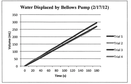
Figure (5.2) - This figure shows the flow rates measured for the bellows pump on 4 different trials These test resulted in an average flow rate of about 96mL/min. The flow rate for the bellows
pump is much steadier than the peristaltic pump. Taking a closer look at the flow rates for each trial in Figure (5.3) below:
Water Flow Rate Through Bellows Pump (2/17/12) 140 - 120 E 100 E 80 - Trial 1 9 60 -nTrial 2 040 OwTrial 3 "- 20 in Trial 4 20 40 60 80 100 120 140 160 180 Time (s)
Figure (5.3) - This figure shows the flow rates at different times during pumping
Water Displaced by Bellows Pump (2/17/12).
350 300 250 --200 - inTrial 1 E .2 150 - a Trial 2 100 - amTrial 3 50 - al Trial 4 50 0 20 40 60 80 100 120 140 160 180 Time (s)
Once again, plotting the flow rate at different points gives more detail on how the pump is behaving. The flow rate varies by no more than about 15mL/min, which is promising. The bellows pump is much more reliable than the peristaltic pump. Further testing needs to be done with both the peristaltic pump and the bellows pump to determine if the pumps will behave the same with a viscous, compressible fluid.
5.2 PRIME TIME
Prime time is how long it takes for the flow to go throughout the system before it actually starts dispensing fluid. The prime time was measured for the peristaltic pump but nothing conclusive was found because the peristaltic pump was unreliable. An important step before moving along would be to repeat these tests, making sure to record the prime time also.
CHAPTER
6
FLUID QUALITY
6.1 QUALITY OF FLUID'
Evaluating the quality of the delivered fluid is paramount for this device. Concerns include:
volume percentage, particle size distribution, oxygen tension, rheometry and degradation. Since
the 90 percent gas by volume, oxygenated fluid is compressible and non-newtonian, it may be
helpful to assess the fluid at a range of concentrations-from 10 percent to 90 percent gas by
volume in 20 percent intervals. This would allow for easy identification of at what concentration
any problems arise.
6.2 VOLUME PERCENTAGE
It is important to confirm that the mixed fluid dispensed by the pump is 70% gas by volume, as it
is one of the functional requirements requested by the client. In order to do this, a defined volume
of fluid within a syringe can be weighed to calculate the volume of the fluid phase, assuming that
the fluid is mostly water so its density is known ( pw,., = 1g / mL ); the mass of an empty syringe
with a cap is 74.56 grams and must be accounted for in calculating the mass of fluid alone. The