Assessing the near surface sensitivity of SCIAMACHY atmospheric CO<sub>2</sub> retrieved using (FSI) WFM-DOAS

(1)

HAL Id: hal-00296284

https://hal.archives-ouvertes.fr/hal-00296284

Submitted on 9 Jul 2007

HAL is a multi-disciplinary open access

archive for the deposit and dissemination of

sci-entific research documents, whether they are

pub-lished or not. The documents may come from

teaching and research institutions in France or

abroad, or from public or private research centers.

L’archive ouverte pluridisciplinaire HAL, est

destinée au dépôt et à la diffusion de documents

scientifiques de niveau recherche, publiés ou non,

émanant des établissements d’enseignement et de

recherche français ou étrangers, des laboratoires

publics ou privés.

atmospheric CO2 retrieved using (FSI) WFM-DOAS

M. P. Barkley, P. S. Monks, A. J. Hewitt, T. Machida, A. Desai, N.

Vinnichenko, T. Nakazawa, M. Yu Arshinov, N. Fedoseev, T. Watai

To cite this version:

M. P. Barkley, P. S. Monks, A. J. Hewitt, T. Machida, A. Desai, et al.. Assessing the near

sur-face sensitivity of SCIAMACHY atmospheric CO2 retrieved using (FSI) WFM-DOAS. Atmospheric

Chemistry and Physics, European Geosciences Union, 2007, 7 (13), pp.3597-3619. �hal-00296284�

(2)

www.atmos-chem-phys.net/7/3597/2007/ © Author(s) 2007. This work is licensed under a Creative Commons License.

Chemistry

and Physics

Assessing the near surface sensitivity of SCIAMACHY atmospheric

CO

2

retrieved using (FSI) WFM-DOAS

M. P. Barkley1,*, P. S. Monks2, A. J. Hewitt1, T. Machida3, A. Desai4, N. Vinnichenko5,†, T. Nakazawa6, M. Yu Arshinov7, N. Fedoseev8, and T. Watai9

1_{EOS, Department of Physics and Astronomy, University of Leicester, UK}

2_{Department of Chemistry, University of Leicester, UK}

3_{National Institute for Environmental Studies, Tsukuba, Japan}

4_{National Centre for Atmospheric Research, Boulder, CO, USA}

5_{Central Aerological Observatory, Dolgoprudny, Russia}

6_{Tohoku University, Sendai, Japan}

7_{Institute of Atmospheric Optics, Tomsk, Russia}

8_{Permafrost Institute, Yakutsk, Russia}

9_{Global Environmental Forum, Tsukuba, Japan}

*_{now at: Institute for Atmospheric and Environmental Science, School of GeoSciences, University of Edinburgh, UK}

†_{deceased 2006}

Received: 30 January 2007 – Published in Atmos. Chem. Phys. Discuss.: 21 February 2007 Revised: 25 April 2007 – Accepted: 29 June 2007 – Published: 9 July 2007

Abstract. Satellite observations of atmospheric CO2offer

the potential to identify regional carbon surface sources and sinks and to investigate carbon cycle processes. The extent to which satellite measurements are useful however, depends on the near surface sensitivity of the chosen sensor. In this pa-per, the capability of the SCIAMACHY instrument on board

ENVISAT, to observe lower tropospheric and surface CO2

variability is examined. To achieve this, atmospheric CO2

retrieved from SCIAMACHY near infrared (NIR) spectral measurements, using the Full Spectral Initiation (FSI) WFM-DOAS algorithm, is compared to in-situ aircraft observations

over Siberia and additionally to tower and surface CO2data

over Mongolia, Europe and North America.

Preliminary validation of daily averaged

SCIA-MACHY/FSI CO2against ground based Fourier Transform

Spectrometer (FTS) column measurements made at Park Falls, reveal a negative bias of about −2.0% for collocated

measurements within ±1.0◦ of the site. However, at

this spatial threshold SCIAMACHY can only capture the variability of the FTS observations at monthly timescales. To observe day to day variability of the FTS observations,

the collocation limits must be increased. Furthermore,

comparisons to in-situ CO2 observations demonstrate that

SCIAMACHY is capable of observing a seasonal signal

Correspondence to: P. S. Monks

(psm7@le.ac.uk)

that is representative of lower tropospheric variability on (at least) monthly timescales. Out of seventeen time series com-parisons, eleven have correlation coefficients of 0.7 or more,

and have similar seasonal cycle amplitudes. Additional

evidence of the near surface sensitivity of SCIAMACHY, is provided through the significant correlation of FSI derived

CO2with MODIS vegetation indices at over twenty selected

locations in the United States. The SCIAMACHY/MODIS comparison reveals that at many of the sites, the amount of

CO2variability is coincident with the amount of vegetation

activity. The presented analysis suggests that SCIAMACHY

has the potential to detect CO2variability within the

lower-most troposphere arising from the activity of the terrestrial biosphere.

1 Introduction

Although water vapour is by far the dominant greenhouse gas, contributing to 60% of the greenhouse effect, its short residence time (∼10 days) means that it is considered as a natural feedback, rather than forcing agent (Kiehl and Tren-berth, 1997). Of the anthropogenic greenhouse gases, carbon

dioxide (CO2) generates the largest forcing and is considered

the principal species with methane (CH4) the next most

(3)

balance is governed by water vapour and clouds, over long time scales (i.e. decades and longer) it is predominately

reg-ulated by CO2. Over the last 200 years there has been a

dra-matic ∼30% rise in atmospheric CO2owing primarily to the

burning of fossil fuels and deforestation. This significant in-crease is likely to have a serious impact on the carbon cycle and climate, as present concentrations are now greater than at any other time in the last half a million years (Siegenthaler et al., 2005).

Two important carbon cycle sinks which absorb CO2from

the atmosphere, and keep levels lower than otherwise, are the terrestrial biosphere and the ocean. The terrestrial

bio-sphere draws down CO2through the creation and

accumula-tion of plant biomass, whereas CO2that diffuses across the

atmosphere-ocean interface is mixed to deep waters by the solubility, biological and carbonates pumps. However, there is much uncertainty about where, and how, this uptake oc-curs. As global carbon emissions show no sign of slowing, the variability and efficiency of the terrestrial and oceanic sinks will play an important role in shaping the Earth’s fu-ture climate. Present estimates of the global carbon cycle fluxes, provided by inverse modelling (e.g. R¨odenbeck et al., 2003; Patra et al., 2006), are restricted by the sparse distribu-tion and limited number of available measurements (Gurney et al., 2002). The greater spatial and temporal coverage of-fered by satellite observations, if of sufficient (∼1%) preci-sion, coupled with inverse models can help identify surface sources and sinks and reduce flux uncertainties (O’Brien and Rayner, 2002; Houweling et al., 2004; Miller et al., 2007). Satellite observations therefore offer an unique ability to in-vestigate the dynamics of the carbon cycle. However, one of

the most important aspects of satellite CO2measurements is

the question of near-surface sensitivity i.e. can the instrument

observe CO2variability within the lower troposphere, where

the signatures of surface fluxes occur?

Thermal infrared sounders, such as AIRS, have limited

sensitivity to surface CO2 as the light that the sensor

de-tects originates from the mid-upper troposphere (Engelen and McNally, 2005; Tiwari et al., 2006). In contrast, NIR instruments such as SCIAMACHY (the only current opera-tional NIR sensor) or the future OCO and GOSAT missions, are sensitive to the lower troposphere since they detect light that is reflected from the Earth’s surface i.e. which has tra-versed the atmospheric path completely. Previous work by Buchwitz et al. (2005a,b, 2006), Houweling et al. (2005) and

Barkley et al. (2006a,b,c) have shown that CO2

measure-ments from SCIAMACHY are possible with a precision that is approaching the 1% threshold requirement for inverse flux modelling (O’Brien and Rayner, 2002) and with an estimated accuracy of a couple of percent.

In this paper, SCIAMACHY CO2, retrieved using the

(FSI) WFM-DOAS algorithm (Barkley et al., 2006a,b,c), is initially validated against ground based Fourier Transform Spectrometer (FTS) column measurements and then

com-pared to in situ aircraft, tower and surface CO2observations

to assess if SCIAMACHY is able to detect changes in

sur-face CO2concentrations. Although SCIAMACHY measures

the CO2column integral, in situ observations of atmospheric

CO2mixing ratios made at the surface or from aircraft can

provide a useful comparison data set. However, care must be taken when performing any analysis. In situ observations occur at a specific location, time and altitude whereas

typi-cally the SCIAMACHY CO2corresponds to a column VMR

which is often given as a monthly gridded product (to im-prove the precision). Thus, a comparison of the magnitudes, phasing and the general behaviour of the seasonal cycle are often the only features that can be examined with any

mean-ing. Thus, validation of SCIAMACHY CO2 using surface

data will, for the most part, be performed using monthly average time series although comparisons to spatially and temporally collocated aircraft measurements over Siberia are demonstrated.

Furthermore, in the second part of this paper, the North American region is selected for a case study. The spatial distributions over this scene for 2003 and 2004 are exam-ined whilst additionally vegetation proxy data, taken from

the MODIS instrument, is compared to SCIAMACHY CO2

at over twenty locations within the U.S. to assess if there is any observable correlation between terrestrial vegetation

ac-tivity and atmospheric CO2concentrations. Any significant

correlation between SCIAMACHY derived CO2 and

vege-tation at specific locations will be further evidence of near surface sensitivity.

This paper is structured as follows. Section 2 contains a brief description of SCIAMACHY whilst Sect. 3 gives an overview of the FSI retrieval algorithm. Validation of

SCIA-MACHY/FSI CO2against ground based FTS measurements

is discussed in Sect. 4 with the detailed comparisons to air-craft, tower and surface measurements performed in Sect. 5. The case study over North America is documented in Sect. 6 with overall conclusions given in Sect. 7.

2 The SCIAMACHY instrument

The SCanning Imaging Absoprtion spectroMeter for Atmo-spheric CHartographY (SCIAMACHY) instrument is a pas-sive UV-VIS-NIR hyper-spectral spectrometer designed to investigate atmospheric composition and processes (Bovens-mann et al., 1999; Gottwald et al., 2006). It was launched onboard the ENVISAT satellite, in March 2002, into a near polar sun-synchronous orbit, from which it can observe the Earth from three viewing geometries: nadir, limb and lu-nar/solar occultation. The instrument measures sunlight that is reflected from the surface or scattered by the atmosphere, covering the spectral range 240–2380 nm (non-continuously) using eight separate grating spectrometers (or channels), with moderate spectral resolution 0.2–1.4 nm. For the ma-jority of its orbit SCIAMACHY make measurements in an alternating limb and nadir sequence. The total columns of

(4)

CO2are derived from nadir observations in the NIR, using a

small micro-window within channel six, centered on the CO2

band at 1.57 µm. For channel 6, the nominal size of each

pixel within the 960×30 km2 (across×along track) swath

is 60×30 km2 which corresponds to an integration time of

0.25 s. Full longitudinal (global) coverage is achieved at the Equator within 6 days.

3 Full Spectral Initiation (FSI) WFM-DOAS

The Full Spectral Initiation (FSI) WFM-DOAS retrieval al-gorithm, discussed in detail in Barkley et al. (2006a,b,c), has

been developed specifically to retrieve CO2 from space

us-ing SCIAMACHY NIR spectral measurements. It is a de-velopment of the WFM-DOAS algorithm first introduced by Buchwitz et al. (2000) whereby the trace gas vertical column density (VCD) can be retrieved through a linear least squares fit of the logarithm of a model reference spectrum I_irefand its

derivatives, plus a quadratic polynomial Pi(am) (i.e. m=2),

to the logarithm of the measured sun normalized intensity

I_imeas: ln I_imeas(Vt) − " ln I_iref( ¯V) +X j ∂ln I_iref ∂ ¯Vj · ( ˆVj− ¯Vj) + Pi(am) # 2

≡ kRESik2 → min w.r.t ˆVj & am (1)

where the subscript i refers to each detector pixel of

cen-tre wavelength λi. The polynomial Pi(am) (which has

co-efficients a0, a1 and a2) is included to account for the

spectral continuum and broadband scattering. The true,

model and retrieved vertical columns are represented by

Vt=(V_COt

2, V t

H2O, V t

Temp), ¯V=( ¯VCO2, ¯VH2O, ¯VTemp) and ˆVj,

respectively (where j refers to the variables CO2, H2O and

temperature). Each derivative represents the change in radi-ance at the top of the atmosphere as a function of a relative scaling of the corresponding trace gas or temperature

pro-file. It should be noted that VTemp is not a vertical column

but rather a scaling factor applied to the vertical temperature

profile. The fit parameters are the trace gas columns ˆVCO2

and ˆVH2O, the temperature scaling factor ˆVTempand the

poly-nomial coefficients am. The error, associated with each of

the fit parameters, is given by Eq. (2) where (Cx)jj refers to

the j th diagonal element from the least squares fit covariance

matrix, RESi is the fit residual, m is the number of spectral

points within the fitting window and n is the number of fit parameters. σ_Vˆ j = s (Cx)jj×PiRES2i (m − n) (2)

The main focus of the FSI algorithm is the inclusion of a priori data within the retrieval in order to minimize the error

associated with the retrieved CO2 column. The FSI

algo-rithm differs from current implementations of WFM-DOAS (e.g. Buchwitz et al., 2005b, 2006) in that rather than us-ing a look-up table approach, it generates a reference spec-trum for each individual SCIAMACHY observation. Each model spectrum is created using the radiative transfer model SCIATRAN (Rozanov et al., 2002), which includes the lat-est version of the HITRAN molecular spectroscopic database (Rothman et al., 2005), from several sources of a priori data including:

– A CO2vertical profile is selected from a specially

pre-pared climatology (Remedios et al., 2006)

– Temperature, pressure and water vapour profiles,

derived from operational 6 hourly ECMWF data (1.125◦×1.125◦grid)

– An approximate value for the surface albedo is inferred

using the mean radiance (within the fitting window) and the solar zenith angle of the SCIAMACHY observation

– Maritime, rural and urban aerosol scenarios are

imple-mented over the oceans, land and urban areas respec-tively using the LOWTRAN aerosol model (Kneizys et al., 1996).

As the line by line calculation of radiances is computation-ally expensive, the FSI algorithm is not implemented on an iterative basis. Instead, each reference spectrum is only used as the best possible linearization point for the retrieval. The potential error from not performing any iterations is kept to a minimum, since the a priori data generate model spectra that closely approximate SCIAMACHY measurements. In order to avoid possible instrumental issues, that hinder re-trievals when using the NIR channels (e.g. Gloudemans et al., 2005), the raw SCIAMACHY spectra (v5.04) are calibrated in-house. Corrections for the orbit specific dark current and detector non-linearity (Kleipool, 2003a,b) are applied. Fur-thermore, a solar spectrum with improved calibration is also used (courtesy of ESA). All SCIAMACHY observations are cloud screened prior to retrieval processing, using the cloud detection method devised by Krijger et al. (2005), with cloud contaminated pixels flagged and disregarded. Back-scans along with observations that have solar zenith angles greater

than 75◦are also not processed. To produce a CO2vertical

column volume mixing ratio (VMR) each retrieved VCD is normalized using the input ECMWF surface pressure. To clean the data from potential biases arising from aerosols or undetected (and partial) cloud contamination only VMRs that have retrieval errors less than 5% and that are within the

range 340–400 ppmv are used. Any CO2column VMRs

(5)

Table 1. Summary of the Park Falls FTS and SCIAMACHY comparison, showing the collocation limits, the number of daily match ups Nc,

the mean bias B and its 1σ standard deviation, the mean column VMRs, MFTSand MSCIAfor the FTS and SCIAMACHY measurements

respectively and their corresponding 1σ standard deviations σFTSand σSCIA, and NFSIwhich is the number of SCIAMACHY observations

used in the calculation of MSCIA. The correlation r between the daily means is given in the last column.

Collocation Limits Nc B σB MFTS σFTS MSCIA σSCIA NFSI r

(lon × lat ) [–] [%] [%] [ppmv] [ppmv] [ppmv] [ppmv] [–] [–] 0.5◦×0.5◦ 13 −3.1 2.6 374.4 2.4 362.8 10.8 4 0.54 1.0◦×1.0◦ 20 −2.1 2.3 374.5 2.1 366.7 9.3 10 0.36 2.0◦×2.0◦ 26 −1.6 1.8 374.3 2.7 368.2 7.7 24 0.49 3.0◦×3.0◦ 29 −1.5 1.6 374.5 2.7 369.1 7.8 40 0.73 4.0◦×4.0◦ 30 −1.3 1.6 374.4 2.7 369.5 7.5 55 0.71 5.0◦×5.0◦ 34 −1.1 1.4 374.4 2.6 370.2 6.8 69 0.71 10.0◦×10.0◦ 40 −0.9 1.3 374.4 2.8 371.0 6.2 208 0.68

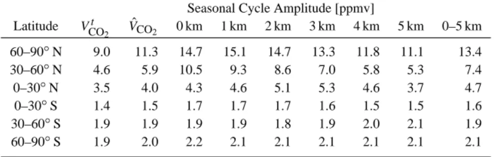
Table 2. Summary of the simulated seasonal cycle amplitudes for the retrieved and true column VMRs, ˆVCO2 and V t

CO2 respectively, in

comparison to the seasonal cycles at the surface and for different altitudes within the lower troposphere when using the CO₂climatology (Remedios et al., 2006). A mean SCIAMACHY averaging kernel has been applied to the true vertical column V_COt

2.

Seasonal Cycle Amplitude [ppmv] Latitude V_COt 2 ˆ VCO2 0 km 1 km 2 km 3 km 4 km 5 km 0–5 km 60–90◦N 9.0 11.3 14.7 15.1 14.7 13.3 11.8 11.1 13.4 30–60◦N 4.6 5.9 10.5 9.3 8.6 7.0 5.8 5.3 7.4 0–30◦N 3.5 4.0 4.3 4.6 5.1 5.3 4.6 3.7 4.7 0–30◦S 1.4 1.5 1.7 1.7 1.7 1.6 1.5 1.5 1.6 30–60◦S 1.9 1.9 1.9 1.9 1.8 1.9 2.0 2.1 1.9 60–90◦S 1.9 2.0 2.2 2.1 2.1 2.1 2.1 2.1 2.1

4 Validation of SCIAMACHY CO2 using Park Falls FTS measurements

Measurements of the CO2column integral by ground based

Fourier Transform Spectrometers (FTS) provide the most

useful means of validating NIR satellite CO2columns (e.g.

Dils et al., 2006). Previous validation of SCIAMACHY/FSI

CO2 to FTS CO2 measurements, made at Egbert (Canada)

revealed a negative bias of about −4% to the measured CO2

concentration (Barkley et al., 2006c). However, the Egbert site is in the region of the large urban centre of Toronto and thus may suffer from local contamination. A more suitable location for satellite CO2validation is the Park Falls site

lo-cated within northern Wisconsin, where existing surface and

tower CO2measurements are already made (e.g. Bakwin and

Tans, 1995). The FTS based at this site, which is part of the

Total Carbon Column Observing Network (TCCON)1, has

already been used to test the OCO retrieval algorithm using SCIAMACHY NIR measurements (B¨osch et al., 2006). The site itself, is surrounded by boreal and wetland forests and relatively flat terrain.

1_{See http://www.tccon.caltech.edu.}

In this paper, measurements of the CO2column made by

Washenfelder et al. (2006) are used to further assess the

ac-curacy of the FSI retrieved CO2. As the FTS measurement

procedure is thoroughly documented in Washenfelder et al. (2006), only a brief outline of the experimental set-up is

given here. The CO2 columns are derived from solar

ab-sorption spectra recorded by a Bruker 125HR FTS housed within a steel shipping container, adjacent to the WLEF TV tower that is situated at the site. The FTS is fully automated with an active solar tracker directing light, from the cen-tre of the solar disk, into the FTS instrument which has a 2.4 mrad field of view. Dual detectors InGasAs and Si-diode detectors then simultaneously record solar spectra over the

interval 3800–15 500 cm−1 at high resolution (0.014 cm−1)

which is sufficient to resolve individual CO2lines.

Simulta-neous retrieval of the CO2 column from two bands centred

at 6228 cm−1 and 6348 cm−1 and of the O2 column from

the band at 7882 cm−1is achieved using the non-linear least

squares spectral fitting (GFIT) algorithm developed at the Jet

Propulsion Laboratory. The CO2dry column average is then

calculated via CO2/O2×0.2095. Under clear sky

observa-tions the measurement precision is 0.1%. Calibration against integrated aircraft profiles indicate a bias of approximately −2.0% but good correlation.

(6)

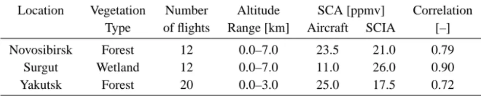
Table 3. Summary of aircraft and SCIAMACHY comparison over Siberia. All values within the table are computed using only coincidental

aircraft and SCIAMACHY observations (i.e. when both measurements occur on the same day). The amplitude of the seasonal cycles (SCA) are shown for SCIAMACHY (denoted SCIA) and for the aircraft over its complete sampling altitude range. The correlation between the aircraft and SCIAMACHY CO2is also shown in the last column.

Location Vegetation Number Altitude SCA [ppmv] Correlation

Type of flights Range [km] Aircraft SCIA [–]

Novosibirsk Forest 12 0.0–7.0 23.5 21.0 0.79

Surgut Wetland 12 0.0–7.0 11.0 26.0 0.90

Yakutsk Forest 20 0.0–3.0 25.0 17.5 0.72

To determine the accuracy of FSI retrieved CO2, daily

av-eraged SCIAMACHY observations, denoted SCIAD,

collo-cated within incremental longitude and latitude limits of the Park Falls site (see Table 1), were directly compared to the

daily mean FTS CO2VMR, denoted P FD, if available. The

bias of each SCIAMACHY CO2column with respect to the

ground based measurement is then given by:

Bias = SCIAD− P FD

P FD

!

× 100% (3)

with the mean bias B, then simply the average over all the SCIAMACHY/FTS match-ups. By applying both the SCIA-MACHY/FSI and the FTS averaging kernels (Fig. 2) to the

CO2climatology, it has been verified that differences in the

CO2columns owing to the different sensitivities of each

in-strument are small: ∼1–2 ppmv.

As Table 1 shows, the bias to the FTS measurements is very dependent on the collocation boundary limits selected around the Park Falls site. At close proximity, i.e. within

0.5◦×0.5◦, the mean bias is −3.1% however the number of

SCIAMACHY/FTS match-ups Nc is small and few

SCIA-MACHY observations, indicated by NFSI, are used to

cal-culate the daily mean. At very large collocation limits

(e.g. 10.0◦×10.0◦) this bias is reduced to only −0.9% owing

both to the greater number of match-ups and the greater

num-ber of SCIAMACHY observations used to calculate SCIAD.

Assuming the errors are random, the precision and accuracy

of SCIAMACHY/FSI CO2 should significantly improve by

the averaging process. This is reflected in the scatter of the

SCIAMACHY data, which is reduced as NFSIincreases. The

negative bias that is found for each of the collocation limits is better than, but consistent with the negative 4.0% offset also observed at Egbert (Barkley et al., 2006c).

For SCIAMACHY observations occurring within

1.0◦×1.0◦ _{of Park Falls (which is the spatial resolution}

of monthly gridded FSI data) the bias is −2.1% but the correlation between the SCIAMACHY and FTS daily means is quite low at 0.36. This implies that SCIAMACHY fails to capture the day to day variability of the FTS measurements. Only once the collocation boundaries are expanded to at

least 3.0◦×3.0◦ (and above) does the correlation become

significant. However, if the 1.0◦×1.0◦limits are again used

but with both data sets assembled into monthly averages then the bias is −2.2% but the correlation improves to 0.94 (which is not attributable to the a priori climatology, see e.g. Figs. 12 and 13). This means that to capture day to day variability around Park Falls (or any FTS site) a wider overpass criteria must be tolerated but to capture monthly

variability collocation limits of 1.0◦×1.0◦ resolution are

acceptable. Either way the bias is about −2.0%.

5 Assessing the near surface sensitivity of SCIA-MACHY

5.1 Model simulations

The SCIAMACHY/FSI averaging kernels peak in the plan-etary boundary layer indicating increased sensitivity to the lower atmosphere (Fig. 2). However, before comparisons be-tween SCIAMACHY and in situ surface data are made, it is necessary to use model simulations to ascertain what one would expect SCIAMACHY to observe as compared to the seasonal signal within the lower troposphere. To achieve this, simulated retrievals were performed using spectra generated

from CO2profiles taken from the newly prepared

climatol-ogy (Remedios et al., 2006). This climatolclimatol-ogy consists of 12

monthly profiles for each 30◦latitude band (see, e.g. Fig. 1

of Barkley et al., 2006a). Initially, a baseline reference spec-trum was created using the U.S. Standard atmosphere with

a uniform a priori CO2 profile scaled to 370 ppmv. Then,

in each retrieval simulation a “measurement” spectrum was

created by inputting into SCIATRAN the climatological CO2

profile (interpolated onto the U.S. Standard pressure scale) along with the U.S. Standard temperature and water vapour profile. The baseline spectrum was then used to perform a synthetic retrieval against each “measurement” with the re-trieved column VMR compared to (a) the true column VMR

of the input climatological CO2profile, calculated after the

application of a SCIAMACHY averaging kernel, and (b) the mixing ratio of the profile at the surface and also at selected altitudes between 0–5 km. Whilst these simulations differ from the FSI approach, which is based on not using fixed a

(7)

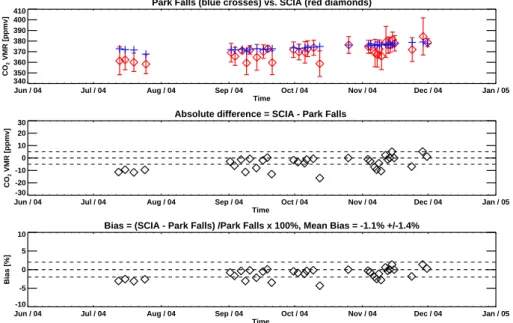
Park Falls (blue crosses) vs. SCIA (red diamonds)

Jun / 04 Jul / 04 Aug / 04 Sep / 04 Oct / 04 Nov / 04 Dec / 04 Jan / 05 Time 340 350 360 370 380 390 400 410 CO 2 VMR [ppmv]

Absolute difference = SCIA - Park Falls

Jun / 04 Jul / 04 Aug / 04 Sep / 04 Oct / 04 Nov / 04 Dec / 04 Jan / 05 Time -30 -20 -10 0 10 20 30 CO 2 VMR [ppmv]

Bias = (SCIA - Park Falls) /Park Falls x 100%, Mean Bias = -1.1% +/-1.4%

Jun / 04 Jul / 04 Aug / 04 Sep / 04 Oct / 04 Nov / 04 Dec / 04 Jan / 05 Time -10 -5 0 5 10 Bias [%]

Fig. 1. Top Panel: The daily mean FTS CO2column measurements (blue crosses) with the corresponding daily average of all SCIAMACHY

measurements (red diamonds) occurring within 5.0◦×5.0◦of the Park Falls site together with its 1σ standard deviation. Middle Panel: The absolute difference (SCIAMACHY minus FTS) between the satellite and ground based observations. The grey dashed lines indicate the ±5 ppmv differences. Bottom Panel: The percentage bias of each SCIAMACHY observation with respect to the FTS measurements. The grey dashed lines indicate the ±2% bias threshold.

priori data, they at least offer some indication of the

differ-ence between column and surface CO2mixing ratios.

The results of these simulations reveal that below 30◦N

the difference between the retrieved column VMR and those at the surface are very similar. In terms of absolute

magni-tudes, the column VMRs below 30◦N are larger than those

mixing ratios at the surface. Furthermore, the magnitude of the seasonal cycles and their phasing of their anomalies (not shown), are almost indistinguishable. Inter-hemispheric mix-ing in the upper troposphere, combined with weaker terres-trial uptake and release at the Southern Hemisphere surface, may both contribute to this finding.

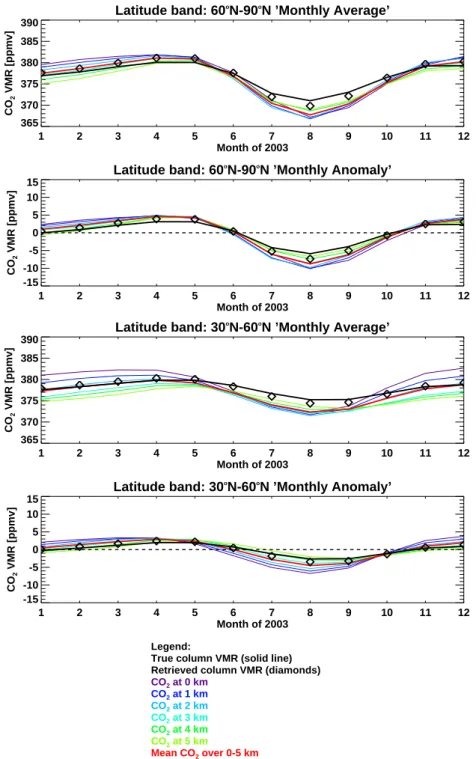
Between 60–90◦N, the phasing between the surface and

column VMRs also agrees well (Fig. 3). This is in spite of the fact the retrieved columns VMRs are lower in the spring months, relative to the mixing ratios at the surface and cor-respondingly higher in the summer months. Furthermore, within this latitude band, the seasonal cycle amplitude of the retrieved column VMRs (11.3 ppmv) is 2.3 ppmv higher than that of true column seasonal amplitude, whereas it is smaller when compared to the seasonal cycle observed at the surface, which is typically ∼14–15 ppmv. The mean amplitude over 0–5 km is however is marginally larger that that of the re-trieved column, 13.4 ppmv as compared to 11.3 ppmv. The over estimation of the true column amplitude within the sim-ulated retrievals originates from the use of a single a priori

CO2profile (Barkley et al., 2006a).

The seasonal cycles between 30–60◦N are similar to those

at higher latitudes with the exception that the phasing of the

retrieved column VMRs slightly lags behind that at the

sur-face at the spring/summer crossover of the CO2 anomaly

(i.e. when photosynthesis exceeds respiration). The delay of the crossover is coherent with the transport and vertical mixing of the seasonal signal from the surface to higher alti-tudes. Within this latitude range, the retrieved column VMR seasonal amplitude is 1.5 ppmv lower than that over 0–5 km but approximately 1 ppmv greater than the true column sig-nal.

Thus, on the basis of these simulations, if one assumes that monthly averaged surface data is adequately representative

of well mixed CO2below 5 km then, at mid to high northern

latitudes, SCIAMACHY should see a seasonal signal smaller than that at the surface but which is in turn larger than that of the true seasonal amplitude of the column integral. More-over, the phasing at high northern latitudes is expected to be consistent with that at the surface whilst at mid-latitudes a slight shift is more likely. In the Southern Hemisphere, the seasonal cycles amplitudes of the column VMRs should be of the same order of those at the surface with approximately the same phasing.

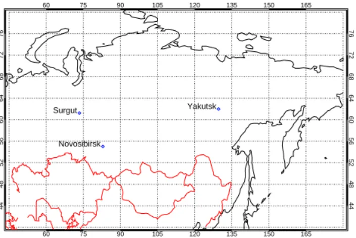
5.2 Comparison to aircraft CO2over Siberia

In this section, SCIAMACHY CO2column VMRs are

com-pared to in-situ volume mixing ratios (denoted as vmrs to distinguish them from column measurements) measured from aircraft flights, made in 2003, over three Siberian

(8)

CO2 volume mixing ratios were determined using the

air-sampling method as outlined in Machida et al. (2001). Over Novosibirsk and Surgut, chartered AN-30 and AN-24 aircraft were used respectively with samples taken by pressurizing air, fed into the cockpit through a drain pipe, into a 0.5 L Pyrex glass flask using a diaphragm pump. These systems were operated manually with the aircraft sampling at eight different altitudes between 0.0–7.0 km over both of these sites. Over Yakutsk, a smaller AN-2 aircraft was used which

only sampled the altitudes 0.0–3.0 km during 2003. The CO2

volume mixing ratios were derived from the flask samples to an accuracy of ∼0.10 ppmv, against standard gases, us-ing a non-dispersive infrared analyzer (NDIR) at either To-hoku University, Japan (for Surgut measurements) or the Na-tional Institute for Environmental Studies (NIES), Japan (for Novosibirsk and Yakutsk measurements). To capture discrete events, SCIAMACHY observations occurring on the same

day of each flight and collocated within ±10.0◦ longitude

and ±8.0◦latitude of each location, were averaged and

com-pared to the mean of the aircraft measurements (convolved with a mean SCIAMACHY averaging kernel) over all sam-pling altitudes.

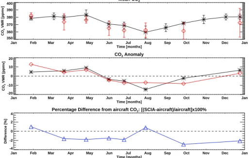
Over Yakutsk, the agreement between the aircraft CO2

vmrs and the column VMRs measured by SCIAMACHY is poor (Fig. 5). However, the aircraft observations agree with SCIAMACHY on the timing and approximate magnitude of

the minimum CO2 at the end of July. The average

differ-ence between SCIAMACHY CO2and the mean aircraft CO2

(over all altitudes) is typically less than 4% with the smallest

difference occurring in July. The CO2anomalies, that is each

measurement minus the mean of its data set, show similar behaviour with the best agreement being between the middle of May to the beginning of July when a significant amount

of CO2 uptake occurs. That said, the minimum of the

air-craft anomaly dips lower than that of SCIAMACHY though the size of the return, between July and October, is approxi-mately the same (8.7 ppmv for SCIAMACHY and 10.7 ppmv for the aircraft observations). The amplitude of the seasonal signal observed by the aircraft varies considerably with alti-tude and has a mean of 25.0 ppmv which is noticeably larger than that detected by SCIAMACHY (17.5 ppmv). The cor-relation between SCIAMACHY and the mean of the aircraft data is 0.72.

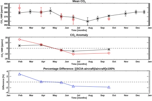
Over Novosibirsk, the overall difference between the mean

aircraft CO2and SCIAMACHY is smaller than at that found

at Yakutsk, only approximately 2% with the correlation 0.77 (Fig. 6). The aircraft data show an extremely large sea-sonal cycle amplitude in the lowest 1 km of >40 ppmv which decreases with altitude. SCIAMACHY observes a smaller seasonal amplitude of 21.0 ppmv which is thus more com-parable to the mean aircraft seasonal amplitude which is 23.5 ppmv. Examination of Fig. 6 reveals that in addition, the

CO2anomalies measured over Novosibirsk show very good

agreement between March–July. The change in the anoma-lies between October and December is also similar.

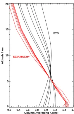
0.2 0.4 0.6 0.8 1.0 1.2 1.4 1.6 Column Averaging Kernel

0 5 10 15 20 Altitude / km SCIAMACHY FTS

Fig. 2. Example averaging kernels, for various solar zenith angles

(i.e. air masses), for SCIAMACHY (red line) and the FTS (black line) highlighting the different sensitivity of each instrument to the lower troposphere. The SCIAMACHY averaging kernels are calcu-lated numerically (see, e.g. Barkley et al., 2006c).

Over Surgut there were only six coincidental SCIA-MACHY observations (Fig. 7). Nevertheless, there is fairly good agreement between SCIAMACHY and the aircraft ob-servations. The volume mixing ratios are of the same order of magnitude and the typical difference from mean aircraft ob-servations is ∼2%. Unlike the measurements over Yakutsk or Novosibirsk, the amplitude of the seasonal cycle detected by SCIAMACHY (26.0 ppmv) is larger than the aircraft obser-vations at any altitude or over any altitude range. At the sur-face, the seasonal amplitude is 19.9 ppmv which decreases rapidly with altitude to only 8.3 ppmv at 7.0 km. Thus, even though a quite strong seasonal cycle is evident at the surface it doesn’t propagate to higher altitudes.

In summary, the FSI retrieved CO2shows fair agreement

to the aircraft observations. Whilst the precision of the raw satellite columns is less than that of the monthly gridded data,

the variation of atmospheric CO2over the selected Siberian

locations is still captured by SCIAMACHY if large colloca-tion limits are used.

5.3 Comparison to in-situ surface observations

5.3.1 Europe and Mongolia

In addition to the aircraft comparison over Siberia,

(9)

Latitude band: 60o N-90o N ’Monthly Average’ 1 2 3 4 5 6 7 8 9 10 11 12 Month of 2003 365 370 375 380 385 390 CO 2 VMR [ppmv] Latitude band: 60o N-90o N ’Monthly Anomaly’ 1 2 3 4 5 6 7 8 9 10 11 12 Month of 2003 -15 -10 -5 0 5 10 15 CO 2 VMR [ppmv] Latitude band: 30o N-60o N ’Monthly Average’ 1 2 3 4 5 6 7 8 9 10 11 12 Month of 2003 365 370 375 380 385 390 CO 2 VMR [ppmv] Latitude band: 30o N-60o N ’Monthly Anomaly’ 1 2 3 4 5 6 7 8 9 10 11 12 Month of 2003 -15 -10 -5 0 5 10 15 CO 2 VMR [ppmv] Legend:

True column VMR (solid line) Retrieved column VMR (diamonds)

CO2 at 0 km CO2 at 1 km CO2 at 2 km CO2 at 3 km CO₂ at 4 km CO₂ at 5 km Mean CO2 over 0-5 km

Fig. 3. Assessment of the near surface sensitivity of SCIAMACHY, for different latitude regions, using the 2003 CO2climatology. The plots

show the the retrieved and true column VMRs against CO2mixing ratios within the lower troposphere both in terms of absolute magnitudes

and also the anomalies.

in-situ observations taken from the World Data Centre for

Greenhouse Gases (WDCGG) network2. In this section this

comparison is confined to Western Europe and to Mongo-lia (since SCIAMACHY retrievals over these region have al-ready been processed for the TM3 model comparison

doc-2_{Downloadable from http://gaw.kishou.go.jp/wdcgg.html}

umented in Barkley et al., 2006c). Within western Europe

there were only five sampling sites which had CO2data for

2003 (shown in Fig. 8) whilst in Mongolia there was only a

single station at Ulann Uul (47◦N, 111◦E). The CO2volume

mixing ratios are measured, on a continuous or weekly basis, at these locations using NDIR analyzers. In this analysis, the monthly averages of the ground based observations have

(10)

60 75 90 105 120 135 150 165 60 75 90 105 120 135 150 165 44 48 52 56 60 64 68 72 76 44 48 52 56 60 64 68 72 76 Yakutsk Surgut Novosibirsk

Fig. 4. The locations of the aircraft flights over Siberia during 2003:

Novosibirsk (55.03◦N, 82.19◦E), Surgut (61.25◦N, 73.41◦E) and Yakutsk (62.00◦N, 129.66◦E).

been used, since the ability of SCIAMACHY to detect sea-sonal variations is being assessed. For this reason, the selec-tion criteria for collocated satellite observaselec-tions was based on

using monthly (1◦×1◦) gridded SCIAMACHY data, with the

average taken of all grid points lying within ±3.5◦latitude

and ±5.0◦ longitude of each site. These collocation limits

were chosen as a compromise between giving the most num-ber of satellite match ups against proximity to the sampling location. The only exception was for the station at Ulaan Uul, which lies within the Gobi Desert. In this case, the monthly average of the whole scene was used, since the region is only

8.0◦×18.0◦wide in the zonal and meridional directions.

Inspection of the time series of the ground based and SCIAMACHY measurements reveals that the in-situ obser-vations are always about 2–4% larger than those observed from space (see Figs. 9 and 10). By only considering the

CO2anomalies against one another this offset, for the most

part, can be effectively removed. Thus, only a comparison

between the CO2anomalies is feasible.

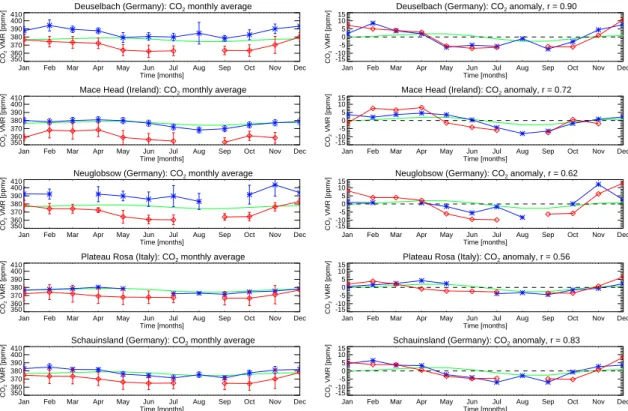
Of all the sampling sites, the Ulann Uul anomaly agrees best with the column VMRs measured by SCIAMACHY. The correlation is 0.95 with the phasing and amplitude of the seasonal cycle matching exceptionally well. More impor-tantly the seasonal cycle that SCIAMACHY observes does not simply follow the input a priori column VMRs (as in-dicated by the green lines in Figs. 9). In addition to Ulann Uul, there is also excellent agreement at Deuselbach and Schauinsland which have correlation coefficients of 0.90 and 0.83, respectively. At Deuselbach, there is especially good agreement between SCIAMACHY and the surface anoma-lies during March–July. Furthermore, over both of these sites SCIAMACHY detects a seasonal cycle amplitude which is approximately the same as that at the surface (Table 4). These locations, which are close to one another, both show a small peak in August. Unfortunately, there aren’t SCIA-MACHY retrievals available for this month, due to

instru-Table 4. Summary of the in-situ ground based comparison over

western Europe, Mongolia and the U.S. The seasonal cycle ampli-tudes (SCA) are given for both the ground based (g-b) and SCIA-MACHY (SCIA) observations. The correlation between the time series is also given. The average correlation using all locations is 0.7.

Location SCA [ppmv] Correlation

g-b SCIA [–]

Surface:

Deuselbach, Germany 15.9 17.7 0.90

Mace Head, Eire 11.1 15.3 0.72

Neuglobsow, Germany 17.6 22.7 0.62

Plateau Rosa, Italy 8.6 10.1 0.56

Schauinsland, Germany 13.4 13.7 0.83

Ulaan Uul, Mongolia 11.5 10.6 0.95

Park Falls, Wisconsin, USA 23.1 17.4 0.72

Niwot Ridge, Colorado, USA 9.6 9.4 0.91

Point Arena, California, USA 13.3 8.3 0.39

Wendover, Utah, USA 9.9 11.7 0.85

Tower:

Argyle, Maine, USA 7.7 30.1 0.19

Park Falls, Wisconsin, USA 18.0 17.4 0.93

Moody, Texas, USA 10.2 9.0 0.50

Sylvania Tower, Michigan, USA 15.9 18.4 0.76

ment decontamination, to corroborate this event. Over Mace Head, Neuglobsow and Plateau Rosa the anomalies agree less well. However, the comparison at both Mace Head and Neuglobsow is hampered as there are fewer SCIAMACHY observations (i.e. surrounding grid points) over theses sta-tion. Mace Head is on the coast, thus a higher number of re-trievals are discarded, whereas Neuglobsow sits on the east-ern edge of the Westeast-ern Europe scene. The lack of grid-ded observations to the east of Neuglobsow clearly affects the agreement between SCIAMACHY and the ground based data. Comprehensive sampling and symmetrical spatial av-eraging of the SCIAMACHY data around each surface site is therefore necessary to avoid the time series being distorted (or influenced) by for example, pollution events, that occur in only one direction relative to the chosen location. Further-more, the Plateau Rosa station is also at a very high altitude (>3 km) within the Italian Alps. The effect of the surface to-pography on the SCIAMACHY retrievals is therefore much greater. Nevertheless, the seasonal amplitude measured at this station is similar to that observed by SCIAMACHY. However, in the spring months there appears to be a notice-able phase shift, with the transition from positive to negative occurring about two and a half months earlier for the ob-served SCIAMACHY signal.

(11)

Mean CO2

Jan Feb Mar Apr May Jun Jul Aug Sep Oct Nov Dec Jan Time [months] 350 360 370 380 390 400 CO 2 VMR [ppmv] CO2 Anomaly

Jan Feb Mar Apr May Jun Jul Aug Sep Oct Nov Dec Jan Time [months] -20 -10 0 10 20 CO 2 VMR [ppmv]

Percentage Difference: [(SCIA-aircraft)/aircraft]x100%

Jan Feb Mar Apr May Jun Jul Aug Sep Oct Nov Dec Jan Time [months] -8 -4 0 4 8 Difference [%]

Fig. 5. The CO2time series over Yakutsk for SCIAMACHY (red) and aircraft (black). Top panel: The mean aircraft CO2mixing ratio

(over all altitudes) and the SCIAMACHY VMRs. The error bars represent the 1σ uncertainty. Second panel: The CO₂anomaly (using only coincidental observations). Third panel: The percentage difference between SCIAMACHY and the mean aircraft CO2mixing ratio (over all

altitudes).

Mean CO2

Percentage Difference from aircraft CO2: [(SCIA-aircraft)/aircraft]x100%

Fig. 6. As Fig. 5 but for the CO2time series over Novosibirsk.

5.3.2 North America

Further to the study outlined in Sect. 5.3.1, a comparison be-tween two consecutive years (2003–2004) of SCIAMACHY

CO2 measurements to WDCGG surface data over North

America was also conducted. Whilst there are numerous operational sampling stations in North America, only four

locations (within the USA) were deemed suitable for this as-sessment. These sites were selected on the basis of having the most number of collocated retrievals to give a more com-plete time series of SCIAMACHY observations. Owing to the much larger scene observed, as compared to Western

Eu-rope, the collocation limits were expanded to ±5.0◦latitude

(12)

Mean CO2

Percentage Difference: [(SCIA-aircraft)/aircraft]x100%

Fig. 7. As Fig. 5 but for the CO₂time series over Surgut.

Of the four sites considered, Niwot Ridge, despite its high altitude, yields the best agreement to SCIAMACHY with a correlation coefficient of 0.91 and a similar seasonal cycle amplitude of ∼9 ppmv (Table 4 and Fig. 12). The phasing between the two observed seasonal cycles is also very sim-ilar. However, at this location the a priori closely follows the surface measurements. Similarly, at Wendover the corre-lation between SCIAMACHY and the surface observations is high and seasonal amplitudes comparable but again the a priori and surface signals are much alike. At Park Falls and Point Arena the agreement is worse. In spite of this, the observations made at Park Falls are important as they demonstrate that SCIAMACHY detects a seasonal signal that is more similar to the surface observations than the a priori (this is also evident for the Park Falls tower measurements shown in Fig. 13). As the surface albedo tends to be higher at Niwot Ridge and Wendover, than at Park Falls, the signal to noise ratio of the SCIAMACHY measurements is better and the FSI retrievals more accurate at these locations. Thus, it is more likely that observed SCIAMACHY signals at Ni-wot Ridge and Wendover are realistic and not simply the case that the retrievals are following the a priori. The poor match at Point Arena is most likely to arise from its coastal location and the constraint that only SCIAMACHY observations over land are considered.

To complement these comparisons, tower data taken from the NOAA/ESRL network and the Sylvania tower, in

Michi-gan, was also evaluated against SCIAMACHY CO2. Each

tower measures the CO2volume mixing ratio at several

dif-ferent heights with a sampling interval, ranging from minutes to hourly, differing between individual sites (see e.g. Bakwin

-24 -20 -16 -12 -8 -4 0 4 8 12 -24 -20 -16 -12 -8 -4 0 4 8 12 44 46 48 50 52 54 56 58 44 46 48 50 52 54 56 58 Deuselbach

Mace Head Neuglobsow

Plateau Rosa Schauinsland

Fig. 8. The surface stations located within the European scene

pro-cessed by the FSI retrieval algorithm.

and Tans, 1995, or Desai et al., 2005). For each tower, CO2

volume mixing ratio was averaged over all the intake heights and then assembled into a monthly mean time series. The only exception was the Sylvania tower, where the maximum intake height (36 m) was used instead. The resultant time se-ries were then compared to SCIAMACHY observations us-ing the same collocation limits as for the surface measure-ments. With the exception of Park Falls, where the correla-tion is 0.92, the agreement between SCIAMACHY and the tower measurements is not noteworthy. This is irrespective of the fact that the magnitude of seasonal cycle amplitudes are very similar (bar the tower at Argyle where a SCIAMACHY outlier in December distorts the amplitude). At Park Falls

(13)

Deuselbach (Germany): CO2 monthly average

Jan Feb Mar Apr May Jun Jul Aug Sep Oct Nov Dec

Time [months] 350 360 370 380 390 400 410 CO 2 VMR [ppmv]

Deuselbach (Germany): CO2 anomaly, r = 0.90

Time [months] -15 -10 -5 0 5 10 15 CO 2 VMR [ppmv]

Mace Head (Ireland): CO2 monthly average

Mace Head (Ireland): CO2 anomaly, r = 0.72

Neuglobsow (Germany): CO2 monthly average

Neuglobsow (Germany): CO2 anomaly, r = 0.62

Plateau Rosa (Italy): CO2 monthly average

Plateau Rosa (Italy): CO2 anomaly, r = 0.56

Schauinsland (Germany): CO2 monthly average

Schauinsland (Germany): CO2 anomaly, r = 0.83

Fig. 9. Time series of ground based European in situ observations (blue) versus SCIAMACHY CO2(red). The 1σ error bars are shown on

the monthly averages.The a priori CO₂column VMR is shown in green.

Ulaan Uul (Mongolia): CO2 monthly average

Ulaan Uul (Mongolia): CO2 anomaly, r = 0.95

Fig. 10. As Fig. 9 but for Ulann Uul, Mongolia.

however, SCIAMACHY agrees with the tower data much

better than with the CO2measurements made at the surface.

For example, there is especially good agreement in the

sum-mer months of 2004 where the changes in the mean CO2

vol-ume mixing ratios are captured well by SCIAMACHY. The strong correlation is most likely a consequence of the fact that the Park Falls tower measurements can be representative of the entire (well-mixed) PBL (Bakwin and Tans, 1995). At

(14)

the Sylvania tower, which is quite close to Park Falls, the correlation is not as strong owing to a slight phase difference relative to the time series of SCIAMACHY observations and

possibly also because of the low CO2intake height. The

in-complete tower time series at Argyle coupled with the sites proximity to the eastern coast contribute to the poor correla-tion with the time series observed by SCIAMACHY.

5.4 Summary

Evaluating the FSI CO2retrievals against the ground based

observations, demonstrates that the column variability ob-served by SCIAMACHY, is similar to changes in surface

CO2 concentrations. Out of the seventeen time series

com-parisons (including those of the aircraft), eleven have corre-lation coefficients of 0.7 or greater and moreover comparable seasonal cycle amplitudes. At locations where the agreement to SCIAMACHY is poor, mitigating circumstances such as high site altitude or proximity to the coast, or scene edge, are the probable cause. Whilst the simulations in Sect. 5.1 sug-gest that SCIAMACHY should see a seasonal signal smaller than that at the surface, observations indicate otherwise. It could be possible that SCIAMACHY is simply over estimat-ing the seasonal cycle, owestimat-ing to some problem with the re-trieval itself. Additionally, at Niwot Ridge and Wendover the a priori is similar to the seasonal signal that SCIAMACHY detects, which might indicate that the retrievals are biased from the input data. However, the phasing and changes in the

CO2anomalies, for example at Deuselbach or the Park Falls

tower where smooth seasonal cycles do not occur, match that well that this cannot be the case. Furthermore, it must be

re-membered that the same a priori CO2data has been used in

the SCIAMACHY retrievals at all these locations. Thus, the good agreement at Ulann Uul, Deuselbach and Niwot Ridge, which have very different seasonal signals, cannot all be at-tributed to the a priori. Hence, it is therefore clear that SCIA-MACHY is apparently sensitive to the lower troposphere and that surface data can be used as a useful validation proxy for satellite column measurements when considering only

varia-tions in the monthly CO2means rather than absolute

magni-tudes.

6 Case study: North America

6.1 Spatial distributions

The two years of SCIAMACHY data processed by the FSI algorithm over North America allows the inter-annual

vari-ability of the retrieved CO2spatial distributions to be

exam-ined (Figs. 14 and 15). Despite using a different set of a

priori data (i.e. 2004 ECMWF fields and a 2004 CO2

cli-matology, instead of 2003 data) within the algorithm, there are quite startling coincidences between monthly scenes of each year. For example, in both years during April a thin

band of high CO2VMRs is witnessed at high latitudes over

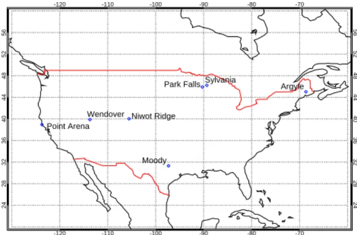
-120 -110 -100 -90 -80 -70 -120 -110 -100 -90 -80 -70 24 28 32 36 40 44 48 52 56 24 28 32 36 40 44 48 52 56 Park Falls Niwot Ridge Point Arena Wendover Argyle Sylvania Moody

Fig. 11. The sampling locations over the USA for (a) sur-face sites: Niwot Ridge (40.03◦N, 105.56◦W, surface altitude

= 3526 m), Point Arena (38.95◦N, 123.72◦W, 17 m) and

Wen-dover (39.88◦N, 113.717◦W, 1320 m) and (b) tower sites: Ar-gyle (45.03◦N, 68.68◦W, surface altitude = 157 m, maximum in-take height = 107 m), Sylvania Tower (46.24◦N, 89.34◦W, 500 m, 36 m) and Moody Tower (31.32◦N, 97.33◦W, 256 m, 457 m). At Park Falls (45.92◦N, 90.27◦W, 868 m, 396.0 m) both surface and tower CO2measurements were available.

Ellesmere Island whilst the position of a small localized

en-hancement over Wyoming (approximately 45◦N, 107◦E) in

2003, is in the same location as a much more widespread

en-hancement in 2004. During May, there are low CO2VMRs

observed over the Appalachian Mountains and southern east-ern states in both 2003 and 2004. By July of each year,

this feature develops into significant band of very low CO2

along the eastern U.S. and also up along the Canadian Shield (though to a lesser extent in 2004). In September, as

vegeta-tion photosynthesis is weakening, the CO2distributions are

much more uniform although there are localized regions of low VMRs e.g. along the Newfoundland Coast or over the Saskatchewan Province in (central) Canada. During October

and November, of both years, the retrieved CO2 fields are

again very uniform.

The regional patterns within the 2003-2004 North

Amer-ica CO2distributions raises several questions. For instance,

are these features real, i.e. do the distributions contain the

signature of surface fluxes? Can the CO2enhancements and

depletions be related to surface processes such as CO2

emis-sions or photosynthetic activity, or are they simply a residual surface albedo effect?

There are two arguments for eliminating a possible dom-inant (seasonal) surface reflectance bias. Firstly, an a priori albedo, determined from the mean radiance of each individ-ual SCIAMACHY observation, is used within the FSI algo-rithm to generate each reference spectrum. A comparison of the monthly gridded a priori surface albedo (not shown) to

the retrieved CO2VMRs reveals that whilst the CO2

(15)

Park Falls (U.S.A.): CO2 monthly average 2003 2004 2005 Time 350 360 370 380 390 400 410 CO 2 VMR [ppmv]

Park Falls (U.S.A.): CO2 anomaly, r = 0.72

2003 2004 2005 Time [months] -20 -10 0 10 20 CO 2 VMR [ppmv]

Niwot Ridge (U.S.A.): CO2 monthly average