HAL Id: hal-03134026
https://hal.archives-ouvertes.fr/hal-03134026
Submitted on 22 Feb 2021HAL is a multi-disciplinary open access archive for the deposit and dissemination of sci-entific research documents, whether they are pub-lished or not. The documents may come from teaching and research institutions in France or abroad, or from public or private research centers.
L’archive ouverte pluridisciplinaire HAL, est destinée au dépôt et à la diffusion de documents scientifiques de niveau recherche, publiés ou non, émanant des établissements d’enseignement et de recherche français ou étrangers, des laboratoires publics ou privés.
Distributed under a Creative Commons Attribution| 4.0 International License
Reconciling carbon-cycle processes from ecosystem to
global scales
Ashley Ballantyne, Zhihua Liu, William Rl Anderegg, Zicheng Yu, Paul Stoy,
Ben Poulter, Joseph Vanderwall, Jennifer Watts, Kathy Kelsey, Jason Neff
To cite this version:
Ashley Ballantyne, Zhihua Liu, William Rl Anderegg, Zicheng Yu, Paul Stoy, et al.. Reconciling carbon-cycle processes from ecosystem to global scales. Frontiers in Ecology and the Environment, Ecological Society of America, 2021, 19 (1), pp.57-65. �10.1002/fee.2296�. �hal-03134026�
Front Ecol Environ 2021; 19(1): 57–65, doi:10.1002/fee.2296
C
arbon (C) is the building block of life. Global photosyn- thesis generates approximately 100 terawatts (TW) of energy each year by converting solar radiation into stored chemical energy (Barber 2009). Photosynthesis also representsthe largest global annual C flux, of ~125 petagrams (Pg; where 1 Pg equals 1015 grams [g] and 1 Pg C is roughly equivalent to
0.47 parts per million [ppm] of CO2), with the second greatest flux consisting of the subsequent release of CO2 via respiration (~122 Pg C/year). Both of these fluxes are an order of magni-tude greater than fossil‐fuel emissions (Ballantyne et al. 2015). The atmospheric CO2 that is fixed during photosynthesis is subsequently stored and transferred as chemical energy, which in turn fuels the metabolic reactions of most autotrophs and heterotrophs. Although C is the most common element in the terrestrial biosphere, representing approximately 50 parts per hundred (%) of all organic matter, CO2 represents only a very small fraction of the atmosphere and is therefore measured in ppm (~415 ppm in 2020). Given the abundance of C in the terrestrial biosphere and the massive fluxes of C occurring between the biosphere and the atmosphere, it is no surprise that scientists have developed a myriad of innovative ways for measuring and simulating C‐cycle processes across a range of scales in time and space. For example, chloroplast CO2 fluxes are estimated over millimeters per second, whereas biome CO2 fluxes may be estimated over thousands of kilometers per year. There have been many advances in C‐cycle science over the past 60 years at leaf, plant, ecosystem, and global scales, but both challenges to and opportunities for scientific advance-ment remain. Progress is necessary, however, especially at the macrosystem scale, where human management and ecological processes are often at odds and create interesting interactions of C dynamics.
One of the greatest impediments to accurate predictions of future climate is the uncertain response of the terrestrial C cycle to impending changes in temperature, precipitation, and atmospheric CO2 concentrations (Friedlingstein et al. 2013). Even though land‐surface models have become increasingly realistic in their mechanistic representation of C‐cycle pro-cesses by including nutrient limitation (Thornton et al. 2007),
Reconciling carbon-cycle processes from
ecosystem to global scales
Ashley P Ballantyne1,2*†, Zhihua Liu3*†, William RL Anderegg4, Zicheng Yu5,6, Paul Stoy7, Ben Poulter8, Joseph Vanderwall1, Jennifer Watts9, Kathy Kelsey10, and Jason Neff11
Understanding carbon (C) dynamics from ecosystem to global scales remains a challenge. Although expansion of global carbon dioxide (CO2) observatories makes it possible to estimate C-cycle processes from ecosystem to global scales, these estimates do not necessarily agree. At the continental US scale, only 5% of C fixed through photosynthesis remains as net ecosystem exchange (NEE), but ecosystem measurements indicate that only 2% of fixed C remains in grasslands, whereas as much as 30% remains in needleleaf forests. The wet and warm Southeast has the highest gross primary productivity and the relatively wet and cool Midwest has the highest NEE, indicating important spatial mismatches. Newly available satellite and atmospheric data can be combined in innovative ways to identify potential C loss pathways to reconcile these spatial mismatches. Independent datasets compiled from terrestrial and aquatic environments can now be combined to advance C-cycle science across the land–water interface.
In a nutshell:
• From a societal perspective, there has never been a more urgent time to advance our understanding of the carbon (C) cycle, given that the atmospheric growth rate of car-bon dioxide (CO2) has reached record levels
• From a scientific perspective, however, there has never been a better time to be a global ecologist, because global C observing systems are becoming more expansive and intensive, allowing scientists to make innovative insights at ecosystem, macrosystem, and global scales
• A fundamental goal of macrosystems research is to rec-oncile important processes from ecosystem to continental scales, which is now achievable using long‐term and con-sistent measurements of C‐cycle dynamics
• Comparisons across scales also reveal many CO2 loss pathways other than respiration that may not be included in ecosystem‐process models
1Department of Ecosystem and Conservation Sciences, University of
Montana, Missoula, MT *([email protected]); 2Laboratoire
des Sciences du Climat et de l’Environnement, Gif-Sur-Yvette, France; 3CAS
Key Laboratory of Forest Ecology and Management, Institute of Applied Ecology, Chinese Academy of Sciences, Shenyang, China; 4School of
Biological Sciences, University of Utah, Salt Lake City, UT; 5Department of
Earth and Environmental Sciences, Lehigh University, Bethlehem, PA;
6Institute for Peat and Mire Research, School of Geographical Sciences,
Northeast Normal University, Changchun, China; 7Department of Biological
Systems Engineering, University of Wisconsin–Madison, Madison, WI;
8National Aeronautics and Space Administration, Goddard Space Flight Center,
Front Ecol Environ doi:10.1002/fee.2296
AP Ballantyne et al.
58 MACROSYSTEMS BIOLOGY
surface hydrology (Wang et al. 2013), and microbial processes (Wieder et al. 2013), this increased complexity does not neces-sarily reduce the range of uncertainty in projections of C uptake among models (eg see Friedlingstein et al. [2006] com-pared to Friedlingstein et al. [2013]). In parallel, there is now a globally nested CO2 observation network that allows for unprecedented measurements of changes in CO2 concentra-tions and fluxes (Schimel et al. 2015). These continuous meas-urements allow estimates to be made of net CO2 exchange from ecosystem to global scales, but not necessarily the under-lying processes that regulate this net exchange (Ciais et al. 2019). In contrast, land‐surface models simulate the underly-ing processes that result in net CO2 exchange, but these are difficult to benchmark due to a lack of process‐level data at the appropriate scale (Luo et al. 2012; Anav et al. 2013).
Although enhanced net C accumulation in the terrestrial biosphere can be inferred from the global C budget, identify-ing the ecosystems in which C is accumulatidentify-ing is still difficult. For example, at the global scale, it can be concluded with con-fidence that ~25% of CO2 emitted to the atmosphere from fossil‐fuel and land‐use emissions has been taken up by the terrestrial biosphere (Ballantyne et al. 2015; Le Quéré et al. 2016), but biomass datasets are too sparse in extent or too short in duration to document which ecosystems continue to accumulate C. More detailed ocean and land measurements now make it possible to identify specific processes affecting the net CO2 atmospheric exchange between the marine biosphere (Landschützer et al. 2015) and terrestrial biosphere (Anderegg
et al. 2015), in some instances at regional scales (Ciais et al.
2019). However, partitioning net C fluxes into their compo-nent gross fluxes of photosynthesis and respiration remains a challenge (Wehr et al. 2016).
Another vexing problem in global C‐cycle research is that top‐down global estimates of net terrestrial C uptake do not agree with bottom‐up ecosystem estimates when integrated globally. For instance, top‐down estimates of global net terres-trial C uptake in 2010 are an order of magnitude less (2.2 ± 2.1 Pg C/year; Ballantyne et al. 2015) than eddy covariance esti-mates up‐scaled globally (22 ± 5 Pg C/year; Jung et al. 2011). Although some of the discrepancy between top‐down and bot-tom‐up estimates of net terrestrial C uptake may be due to issues associated with eddy covariance methods (Keenan et al. 2019) – particularly regarding measurement of nighttime respi-ration, which often violates eddy covariance requirements of turbulent flux and biases in the sampling network – a portion can also be explained by non‐respiratory CO2 loss pathways (~7 Pg C/year; Randerson et al. 2002). This suggests that there are many C transformation and transport pathways that ultimately lead to a loss of CO2 from ecosystems back to the atmosphere. Approximately 90% of inland lakes and streams are net sources of CO2 to the atmosphere (Cole et al. 1994), and at a global scale approximately 2 Pg C/year is returned to the atmosphere via CO2 loss from rivers and lakes (Raymond et al. 2013). Although this estimate of CO2 loss from aquatic ecosystems is comparable to the magnitude of net C uptake by terrestrial ecosystems, it is
less than 2% of total inferred CO2 respiration from the terres-trial biosphere back to the atmosphere (Ballantyne et al. 2017). As such, characterizing the C balance at the macrosystem scale for direct comparison with different biomes in Earth system models remains difficult (Peylin et al. 2013).
Although from a societal perspective there has never been a more urgent time to study the C cycle and its sensitivity to climate change (Obama 2017), from a scientific perspective there has never been a more exciting time to study C‐cycle processes. The global C observation network supports inno-vative analyses and syntheses across scales from ecosystems to the entire planet. Currently, there are over 800 eddy covari-ance sites operating around the world that contribute meas-urements of net CO2 exchange, as well as estimates of primary productivity and total respiration across a wide array of eco-systems (Chu et al. 2017). However, in the US, fewer than half of the ecosystem functional types are represented in the com-bined core sites of the AmeriFlux Network and the National Ecological Observatory Network (NEON) (Villarreal et al. 2018), and many ecosystems remain underrepresented, espe-cially in climate‐sensitive Arctic tundra and tropical rainfor-ests. Other C flux databases have continued to expand, such as a recently updated database on soil respiration that has been used to identify the climate sensitivity of soil respiration over time (Bond‐Lamberty and Thomson 2010), which is critical for evaluating how C supply, soil temperature, and moisture interact to regulate soil respiration (Hursh et al. 2017).
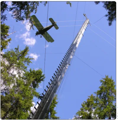
Global measurement networks and satellite observations of atmospheric CO2 now allow for the characterization of biome‐ scale C fluxes at greater temporal and spatial resolutions (Figure 1). The global greenhouse observation network has grown sporadically, with approximately 90 in situ sites now in operation worldwide (GLOBALVIEW‐CO2 1999). Several of these sites also provide atmospheric profile measurements that are essential for estimating latitudinal differences in CO2 exchange (Stephens et al. 2007), in addition to seasonal differ-ences in regional uptake (Gatti et al. 2014). Regional atmos-pheric CO2 monitoring networks often engage in intensive atmospheric campaigns to better define regional C fluxes in urban continental settings (Corbin et al. 2010) or to determine recent changes in the C balance of ecosystems in climate sensi-tive regions, such as the Arctic (Commane et al. 2017). When combined with three‐dimensional atmospheric transport modeling and estimates of surface fossil‐fuel emissions, these so‐called “atmospheric inversions” deliver critical information about the net exchange of CO2 at biome scales (Peylin et al. 2013). The array of Earth observing satellites has also grown tremendously, providing better spatiotemporal coverage of vegetation indices that are useful for assessing patterns and trends of global productivity since ~1982 (Pinzon and Tucker 2010), as well as valuable information on changes in vegetation cover (Song et al. 2018) and ecosystem stress (Anderegg
et al. 2018). Recent advances in satellite observations facilitate
quantification of concentration estimates integrated over the entire total atmospheric column for CO2 (ie XCO2) and
CH4 (ie XCH4). Although potentially less precise than those relying on surface measurements using infrared gas analyzers, these estimates provide more continuous global coverage, improving characterization of regional flux anomalies and attribution to specific C‐cycle processes (Liu et al. 2017).
Innovative ways to combine ecosystem measurements with satellite observations have made it possible to quantify how different ecosystems are responding to concomitant changes in atmospheric composition, including CO2 concentration, sur-face temperatures, and regional precipitation. Moreover, these top‐down and bottom‐up observations are helping researchers to disentangle net C exchange into its component processes of photosynthesis and respiration across various scales, which provides important diagnostics for models that are designed to simulate the concurrent ecological processes and not just net CO2 exchange. For instance, combined satellite and meteoro-logical observations have been used in a machine‐learning framework to up‐scale eddy covariance measurements to pro-vide spatially and temporally continuous estimates of global primary productivity (Jung et al. 2011). Likewise, global atmospheric CO2 measurements have been used to constrain net CO2 exchange in combination with satellite data to con-strain primary productivity to infer the uncoupling of photo-synthesis and respiration on decadal timescales (Ballantyne et
al. 2017). The challenge for the scientific community is
figur-ing out ways in which emergent patterns of net CO2 exchange can be used (Cox et al. 2013) to identify underlying mechanis-tic processes that can be diagnosed in models (Anderegg et al. 2015). Ultimately, this will lead to scientific advances and societal benefits through improved Earth system models with less uncertainty in future climate predictions.
Theoretical representation of C‐cycle processes
Although the global C observing system has been greatly expanded and advanced over the past six decades, the the-oretical and conceptual framework for understanding C‐cycle dynamics has not necessarily kept pace (Figure 2). There has been extensive discussion over the past several decades concerning how the biosphere–atmosphere C exchange can best be defined. The challenges in defining C exchange lie across several axes, including time, space, and C form. Additional issues arise from the different processes occurring in and the transfer of C between aquatic and terrestrial ecosystems. Although we focus solely on terrestrial processes occurring from the ecosystem to biome scale here, we acknowledge the importance of the aquatic interface (Butman
et al. 2018). The evolution of C‐cycle measurements and
key issues regarding terminology was described by Chapin
et al. (2006), who defined net ecosystem C balance (NECB)
simply as the change in C per unit time, but then broke this measure down into its component fluxes:
In this formulation, net ecosystem exchange (NEE) is a measure of the net ecosystem CO2 exchange as the difference between gross primary productivity (GPP) and total eco-system respiration (TER), and at the ecoeco-system scale is typically measured using eddy covariance techniques (Wofsy
et al. 1993). Although the CO2 flux associated with NEE is usually the dominant form of net C exchange in many ecosystems, it cannot be assumed that transformations of C do not occur as a result of ecosystem processes. For instance, fluxes of carbon monoxide (FCO), volatile organic compounds (FVOC), methane (FCH4), dissolved inorganic C (FDIC), dissolved organic C (FDOC), and particulate C (FPC) all represent C loss pathways that may affect the net C balance over time. Although NEE is sometimes used syn-onymously with NECB, it is an approximation that can, under certain circumstances, leave out quantitatively impor-tant non‐respiratory processes that contribute to ecosystem C balance.
A second key issue in C balance terminology emerges at larger spatial or temporal scales when other factors can become major contributors to C balance. Notably, large distur-bances like wildfire, landslides, and insect infestations can cause large or punctuated redistributions of C. In human man-aged ecosystems, activities such as logging, harvest, and other forms of C transfer can result in C taken up at the ecosystem scale being lost at the biome scale, and this transfer can actually cause NECB to shift from a net C sink to a net C source. The net biome productivity (NBP) concept was first introduced by Schulze et al. (2000) to account for C transfer and subsequent (Equation 1).
NECB = NEE − FCO− FVOC− FCH4− FDIC− FDOC− FPC
Figure 1. Image of airborne observations combined with eddy flux obser-vations of carbon (C) fluxes to measure ecosystem–atmosphere exchanges of carbon dioxide (CO2).
A V ar la gin/im ag ge o.egu .eu
Front Ecol Environ doi:10.1002/fee.2296
AP Ballantyne et al.
60 MACROSYSTEMS BIOLOGY
loss at regional scales. In Chapin et al. (2006), NECB represents NBP integrated over fixed space and time domains, with the assumption that additional processes analogous to those shown in Equation (1) may need to be added to account for C fluxes driven by periodic events. At the global scale, we can assume that CO2 mass is conserved in the atmosphere and thus, given fossil‐fuel emissions to the atmosphere and esti-mates of net CO2 uptake by the oceans, net CO2 uptake by the terrestrial biosphere can be inferred (Le Quéré et al. 2016). More importantly, the atmosphere and oceans provide con-straints on global C exchange because these are relatively well‐ mixed homogenous reservoirs as compared to ecosystem C pools and fluxes that tend to be much more spatially and tem-porally heterogeneous. Resolving C‐cycle processes from eco-system to global scales may therefore require an update to C‐cycle nomenclature (see WebPanel 1).
Spatial scale differences in C balance
The “C exchange efficiency” (CEE = NEE/GPP) may provide a useful framework (see WebFigure 1) for comparing relative fluxes across ecosystem to global scales. At the global scale, only ~2% of C fixed annually through GPP remains in the biosphere as a result of NEE (2.5/125 Pg C/year), suggesting that CEE of the terrestrial biosphere is remarkably low. At the scale of the continental US, approximately 5% of C fixed annu-ally through photosynthesis remains in the terrestrial biosphere (Figure 3). However, estimates of CEE derived from eddy
covariance methods reveal very large differences among terrestrial ecosystems. Ecosystems with lower levels of GPP tend to fall on the CEE line at the continental scale, whereas more pro-ductive ecosystems tend to deviate from the CEE line. For example, grasslands have very low CEE (~2%), a level consistent with the global CEE, whereas evergreen needleleaf forests and deciduous broadleaf forests appear to have quite high CEE values (~31% and ~24%, respec-tively). Therefore, our ecosystem‐scale measure-ments suggest that these forests are strong C sinks, whereas our global‐scale measurements suggest that much of this apparent forest C uptake is lost, indicating that these forests may be acting more like “C sieves”. Moreover, crop-lands vary considerably, with less productive croplands falling on the continental CEE line and more productive croplands deviating con-siderably, with an overall CEE of 23%. It should be noted, however, that according to mass bal-ance, the integral of NEE across all ecosystems (aquatic and terrestrial) should be equal to global NEE; in other words, CEE estimates from the different ecosystems shown in Figure 3 should all fall on the continental CEE line (Chapin et
al. 2006). Therefore, measurements of net CO2 exchange at the ecosystem scale are biased, or CO2 loss pathways at the continental scale are offsetting the apparent net uptake of CO2 by certain ecosystems.
Measurement biases of ecosystem C fluxes stem from the location of eddy flux sites or systematic biases in NEE measure-ments. In the US, this network bias should be reduced with the addition of more observation sites, such as NEON sites; however, there remain notable gaps in the intermountain west, north‐ central plains, and parts of the Southeast. Also noteworthy is that eddy flux sites are often situated in rapidly regenerating ecosys-tems and as such may not capture the full trajectory of ecosystem C dynamics (Luyssaert et al. 2008). Furthermore, the eddy flux approach only measures the net ecosystem CO2 exchange (ie NEE) directly, whereas photosynthetic fluxes and total ecosys-tem respiration fluxes are estimated, resulting in the potential for systematic biases to occur in these measurements. Eddy covari-ance methods are inherently challenging in ecosystems with dense canopies (Thomas et al. 2013), which can lead to nocturnal C storage within the canopy (Fu et al. 2018) and decoupling of the canopy and the atmosphere that may vary seasonally (Jocher
et al. 2017). This may help explain the strong divergence between
both deciduous broadleaf and evergreen needleleaf forests and the CEE line at the continental scale (Figure 3). If daytime respi-ration is reduced with respect to nighttime respirespi-ration, large overestimates of both photosynthetic gains and respiration losses at the ecosystem scale may result, which would increase relative ecosystem CEE (Keenan et al. 2019).
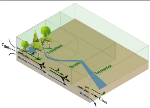
Figure 2. Conceptual figure showing pathways of C gain and loss from ecosystem to biome to terrestrial scales within the biosphere. Although it is often assumed that very little change occurs among the gas, particulate, and dissolved phases of C, ecosystems are very effective at transforming C, such that C gain pathways may not correspond with C loss pathways, leading to an apparent C imbalance across scales. Furthermore, C can be transported across scales via either advection through the atmosphere or fluvial processes in aquatic ecosystems.
The discrepancy between CEE at the biome scale and the ecosystem scale can also be explained by the lack of measurements of non‐ respiratory loss pathways of CO2 back to the atmosphere (Figure 2). For example, aquatic ecosystems, which are effective at transporting dissolved and particulate forms of inorganic and organic C and transforming it to CO2 such that it may be lost to the atmosphere (Neff and Asner 2001; Hotchkiss et al. 2015), were not plotted on our diagnostic CEE plot (Figure 3). There are many measurements of the partial pressure of CO2 in aquatic environments, which determine whether CO2 is diffusing in or out of aquatic ecosystems, but these are not always combined with productivity estimates (albeit see Hotchkiss et al. 2015; Bernhardt et
al. 2018). Volatile organic C (VOC) compounds
are another major source of C loss from eco-systems, which may help to reconcile the dis-crepancy between ecosystem‐ and biome‐scale C exchange efficiencies. Estimates of VOC production are tightly coupled to primary pro-ductivity and range around 450 teragrams (Tg) C/year, making them a very small fraction of terrestrial GPP (less than 0.4%) but an appreci-able fraction of NEE (~15%), assuming that VOCs are rapidly oxidized to form CO2 (Unger
et al. 2013). Finally, the only ecosystem‐scale C
loss pathways that can help reconcile
ecosys-tem‐ and global‐scale estimates of CEE are oxidative pathways that ultimately lead to atmospheric CO2 (eg CO2 emissions from wildfires), meaning that other loss pathways leading to reduced C (eg CH4 emissions) will not help reconcile these discrepancies of scale.
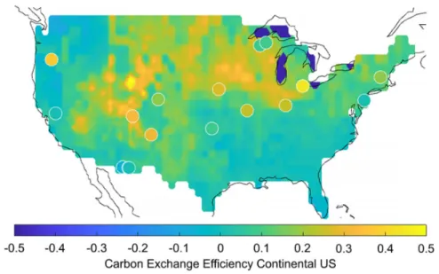
We can also look at the spatial distribution of CEE from the biome to ecosystem scale (Figure 4). At the continental scale in the US, it is apparent that high CEE in the midwestern region near the Great Lakes is driven primarily by high mean annual NEE, and very high CEE in the intermountain west is driven by low GPP and modest NEE. In contrast, highly pro-ductive regions, such as the Pacific Northwest and the Southeast, do not necessarily retain a large fraction of GPP as NEE, as reflected in their relatively low CEE values. These regional differences in CEE seem to be corroborated by eddy covariance sites in certain biomes, such as the Northeast and parts of the Southwest, but less so in other regions. There appears to be a strong mismatch in CEE near the Great Lakes, with regional estimates suggesting a relatively high CEE, whereas eddy flux sites indicate a much lower CEE. This may be due to the specific locations of eddy flux sites that may not capture the diverse array of midwestern ecosystems. A similar mismatch is evident in the Pacific Northwest, where regional CEE values are extremely low – and in some instances nega-tive – due to an apparent net source of CO2 to the atmosphere,
while eddy flux measurements from central Oregon suggest high CEE.
Climate sensitivity of C‐cycle processes
At the continental scale in the US, mean annual primary productivity and net CO2 exchange do not necessarily covary spatially and appear to occupy different climate spaces at regional scales (Figure 5; Liu et al. 2018). GPP is highest in the relatively warm and wet Southeast (Figure 5a), correspond-ing with high levels of mean annual precipitation (MAP, >1200 mm) across a range of mean annual temperatures (MAT, ~10–20°C; Figure 5c). In contrast, NEE is more variable, with the highest values in the Midwest (Figure 5b) at intermediate to high levels of MAP (~750–1200 mm) and lower MAT (<10°C) (Figure 5d). The spatial covariance of GPP and NEE becomes decoupled as water availability increases. We found a strong precipitation threshold of ~700 mm/year over the continental US, below which NEE is regulated by photosyn-thetic gains and above which NEE is regulated to a greater degree by respiration losses (Liu et al. 2018). This result is consistent with ecosystem‐scale studies that show the greatest response in productivity to precipitation anomalies in semi‐ arid grassland and shrubland ecosystems (Knapp and Smith 2001). However, the lateral transport of C through river flow
Figure 3. Comparison of C exchange efficiency (CEE) at ecosystem to biome scales across the continental US. Each point represents the mean annual gross ecosystem productivity and total ecosystem respiration for cropland (CRO), deciduous broadleaf forests (DBF), evergreen needleleaf (ENF), grassland (GRA), mixed forest (MF), open shrubland (OSH), and woody savanna (WSA) eddy covariance sites across the US. The diagonal line was derived from satel-lite estimates of gross primary productivity (GPP) and atmospheric estimates of net CO2 exchange at the scale of the continental US and indicates that 95% of C fixed during photosyn-thesis is lost to the atmosphere through respiration, or that CEE is only 5% (1 – 0.95 = 0.05), represented by the green wedge.
Front Ecol Environ doi:10.1002/fee.2296
AP Ballantyne et al.
62 MACROSYSTEMS BIOLOGY
and human harvest may also be important in uncoupling GPP from NEE at continental scales. This spatial mismatch is an important finding because it is often assumed that anomalies in photosynthesis directly result in anomalies in net CO2 exchange. In fact, it is impossible in standard eddy covariance approaches for partitioning fluxes to have increases in net exchange without increases in photosynthesis (Reichstein et al. 2005), and net C exchange in land‐surface models is dominated by pho-tosynthetic inputs (Liu et al. 2018).
At the global scale, the relationship between the interannual variability of the atmospheric CO2 growth rate and tropical land‐surface temperatures has been identified as an emer-gent constraint, such that higher surface tem-peratures diminish NEE (Cox et al. 2013). However, identifying the processes associated with this diminished NEE is difficult because increased tropical temperatures suppress pho-tosynthesis and/or promote respiration, both of which lead to reduced net C exchange. It has been suggested that total respiration is the
Figure 4. CEE for the continental US. Spatially continuous estimates of GPP derived from Moderate Resolution Imaging Spectroradiometer (MODIS) satellite estimates and continuous estimates of net ecosystem exchange derived from atmospheric inversions over the continen-tal US (Peters et al. 2007) are compared with in situ ecosystem-scale measurements made at 16 different eddy covariance core sites within the AmeriFlux Network (circle points). Positive values indicate regions where ecosystems are a net sink of C from the atmosphere, whereas negative values indicate regions where ecosystems are a net source of C to the atmosphere.
Figure 5. Continental-scale estimates of mean annual GPP and net CO2 exchange (ie NEE) and their sensitivities to climate factors. (a) Continental-scale estimates of GPP from MODIS satellite observations plotted within (c) their climate space of mean annual precipitation and mean annual temperature. (b) Continental-scale estimates of NEE from atmospheric CO2 inversion methods plotted within (d) their climate space. All flux estimates are reported as g C/m2/year and have been projected to ecosystem area (modified from Liu et al. [2018]; see WebTable 1).
(a) (b)
most likely mechanism explaining the emergent relationship between interannual variability in the atmospheric growth rate and tropical surface temperature (Anderegg et al. 2015) and that water limitation is important in regulating net CO2 exchange at the local scale, whereas temperature becomes more important at global scales (Jung et al. 2017). Recent satel-lite evidence suggests that terrestrial water availability that integrates temperature and precipitation variability may be the ultimate mechanism regulating interannual NEE at the global scale (Humphrey et al. 2018). However, evidence derived from satellite estimates of XCO2 and solar induced fluorescence during the recent 2015/2016 El Niño event suggest that net tropical C uptake was reduced by different processes in differ-ent tropical regions – such as reduced photosynthesis in South America, increased respiration in Africa, and increased fire emissions in Southeast Asia (Liu et al. 2017). Therefore, even though we are gaining new insight on the climate sensitivity of important C‐cycle processes, ecosystem‐scale observations are still lacking in certain regions to help reconcile different C‐cycle processes operating at different spatial scales.
Conclusions and frontiers in C‐cycle research
A central goal of ecology at the macrosystem scale is to understand biosphere processes and their complex interactions with climate, land use, and changes in species distribution at regional to continental scales This has also been a central challenge of C‐cycle research because there is a long history of atmospheric CO2 observations that have enabled a better understanding of the C cycle at the global scale and a network of eddy covariance measurements of CO2 exchange at the ecosystem scale. However, reconciling differences in net CO2 exchange measured at these different scales continues to be difficult. We are now acquiring data from aircraft and satellites that allow important C‐cycle processes to be resolved at the biome scale. The terrestrial and aquatic ecological research communities are also compiling databases to elucidate impor-tant C‐cycle processes that may be merged to provide an integrated understanding of C transport and transformations across watersheds. Collectively, we are identifying missing pieces of the global C puzzle that now make it possible to reconcile and understand processes that help to explain dis-crepancies in C dynamics across scales.
Acknowledgements
Publication of this Special Issue was funded by the US Na-tional Science Foundation (NSF award number DEB 1928375). APB was supported by the NSF Macrosystems Biology Pro-gram (1802810). ZL acknowledges support from the National Natural Science Foundation of China (41922006) and the KC Wong Education Foundation. PS acknowledges support from NSF (1552976, 1632810, 1702029) and the US Depart-ment of Agriculture National Institute of Food and Agriculture (USDA NIFA) Hatch project 228396. WRLA was supported
by the David and Lucille Packard Foundation, NSF grants 1714972 and 1802880, and the USDA NIFA Agricultural and Food Research Initiative Competitive Program, Ecosystem Services and Agro‐ecosystem Management (2018‐67019‐ 27850). BP acknowledges support from the National Aeronautics and Space Administration Terrestrial Ecology Program.
References
Anav A, Friedlingstein P, Kidston M, et al. 2013. Evaluating the land and ocean components of the global carbon cycle in the CMIP5 Earth system models. J Climate 26: 6801–43.
Anderegg WRL, Ballantyne AP, Smith WK, et al. 2015. Tropical nighttime warming as a dominant driver of variability in the ter-restrial carbon sink. P Natl Acad Sci USA 112: 15591–96.
Anderegg WRL, Konings AG, Trugman AT, et al. 2018. Hydraulic diversity of forests regulates ecosystem resilience during drought. Nature 561: 538–41.
Ballantyne AP, Andres R, and Houghton R. 2015. Audit of the global carbon budget: estimate errors and their impact on uptake uncer-tainty. Biogeosciences 12: 2565–84.
Ballantyne A, Smith W, Anderegg W, et al. 2017. Accelerating net terrestrial carbon uptake during the warming hiatus due to reduced respiration. Nat Clim Change 7: 148.
Barber J. 2009. Photosynthetic energy conversion: natural and artifi-cial. Chem Soc Rev 38: 185–96.
Bernhardt ES, Heffernan JB, Grimm NB, et al. 2018. The metabolic regimes of flowing waters. Limnol Oceanogr 63: S99–118.
Bond‐Lamberty B and Thomson A. 2010. Temperature‐associated increases in the global soil respiration record. Nature 464: 579–82. Butman DE, Striegl RG, Stackpoole SM, et al. 2018. Inland waters. In:
Cavallaro N, Shrestha G, Birdsey R, et al. (Eds). Second State of the Carbon Cycle Report (SOCCR2): a sustained assessment report. Washington, DC: US Global Change Research Program. Chapin FS, Woodwell GM, Randerson JT, et al. 2006. Reconciling carbon‐
cycle concepts, terminology, and methods. Ecosystems 9: 1041–50. Chu H, Baldocchi DD, John R, et al. 2017. Fluxes all of the time? A
primer on the temporal representativeness of FLUXNET. J Geophys Res-Biogeo 122: 289–307.
Ciais P, Tan J, Wang X, et al. 2019. Five decades of northern land car-bon uptake revealed by the interhemispheric CO2 gradient.
Nature 568: 221–25.
Cole JJ, Caraco NF, Kling GW, and Kratz TK. 1994. Carbon dioxide supersaturation in the surface waters of lakes. Science 265: 1568–70. Commane R, Lindaas J, Benmergui J, et al. 2017. Carbon dioxide
sources from Alaska driven by increasing early winter respiration from Arctic tundra. P Natl Acad Sci USA 114: 5361–66.
Corbin KD, Denning AS, Lokupitiya EY, et al. 2010. Assessing the impact of crops on regional CO2 fluxes and atmospheric
concen-trations. Tellus B 62: 521–32.
Cox PM, Pearson D, Booth BB, et al. 2013. Sensitivity of tropical car-bon to climate change constrained by carcar-bon dioxide variability. Nature 494: 341–44.
Friedlingstein P, Cox P, Betts R, et al. 2006. Climate–carbon cycle feedback analysis: results from the C4MIP model intercompari-son. J Climate 19: 3337–53.
Front Ecol Environ doi:10.1002/fee.2296
AP Ballantyne et al.
64 MACROSYSTEMS BIOLOGY
Friedlingstein P, Meinshausen M, Arora VK, et al. 2013. Uncertainties in CMIP5 climate projections due to carbon cycle feedbacks. J Climate 27: 511–26.
Fu Z, Gerken T, Bromley G, et al. 2018. The surface–atmosphere exchange of carbon dioxide in tropical rainforests: sensitivity to environmental drivers and flux measurement methodology. Agr Forest Meteorol 263: 292–307.
Gatti LV, Gloor M, Miller JB, et al. 2014. Drought sensitivity of Amazonian carbon balance revealed by atmospheric measure-ments. Nature 506: 76–80.
GLOBALVIEW‐CO2. 1999. Cooperative atmospheric data integra-tion project – carbon dioxide. Boulder, CO: Naintegra-tional Oceanic and Atmospheric Administration.
Hotchkiss ER, Hall Jr RO, Sponseller RA, et al. 2015. Sources of and processes controlling CO2 emissions change with the size of streams and rivers. Nat Geosci 8: 696.
Humphrey V, Zscheischler J, Ciais P, et al. 2018. Sensitivity of atmos-pheric CO2 growth rate to observed changes in terrestrial water storage. Nature 560: 628–31.
Hursh A, Ballantyne A, Cooper L, et al. 2017. The sensitivity of soil respiration to soil temperature, moisture, and carbon supply at the global scale. Glob Change Biol 23: 2090–103.
Jocher G, Ottosson Löfvenius M, De Simon G, et al. 2017. Apparent winter CO2 uptake by a boreal forest due to decoupling. Agr Forest
Meteorol 232: 23–34.
Jung M, Reichstein M, Margolis HA, et al. 2011. Global patterns of land–atmosphere fluxes of carbon dioxide, latent heat, and sensi-ble heat derived from eddy covariance, satellite, and meteorologi-cal observations. J Geophys Res-Biogeo 116: G00J07.
Jung M, Reichstein M, Schwalm CR, et al. 2017. Compensatory water effects link yearly global land CO2 sink changes to temperature. Nature 541: 516–20.
Keenan TF, Migliavacca M, Papale D, et al. 2019. Widespread inhi-bition of daytime ecosystem respiration. Nature Ecol Evol 3: 407–15.
Knapp AK and Smith MD. 2001. Variation among biomes in temporal dynamics of aboveground primary production. Science
291: 481–84.
Landschützer P, Gruber N, Haumann FA, et al. 2015. The reinvigora-tion of the Southern Ocean carbon sink. Science 349: 1221–24. Le Quéré C, Andrew RM, Canadell JG, et al. 2016. Global carbon
budget 2016. Earth Syst Sci Data 8: 605–49.
Liu J, Bowman KW, Schimel DS, et al. 2017. Contrasting carbon cycle responses of the tropical continents to the 2015–2016 El Niño. Science 358: eaam5690.
Liu Z, Ballantyne AP, Poulter B, et al. 2018. Precipitation thresholds regulate net carbon exchange at the continental scale. Nat Commun 9: 3596.
Luo YQ, Randerson JT, Friedlingstein P, et al. 2012. A framework for benchmarking land models. Biogeosciences 9: 3857–74.
Luyssaert S, Schulze E‐D, Börner A, et al. 2008. Old‐growth forests as global carbon sinks. Nature 455: 213–15.
Neff JC and Asner GP. 2001. Dissolved organic carbon in terrestrial ecosystems: synthesis and a model. Ecosystems 4: 29–48.
Obama B. 2017. The irreversible momentum of clean energy. Science
355: 126–29.
Peters W, Jacobson AR, Sweeney C, et al. 2007. An atmospheric per-spective on North American carbon dioxide exchange: CarbonTracker. P Natl Acad Sci USA 104: 18925–30.
Peylin P, Law RM, Gurney KR, et al. 2013. Global atmospheric car-bon budget: results from an ensemble of atmospheric CO2
inver-sions. Biogeosciences 10: 6699–720.
Pinzon JE and Tucker CJ. 2010. GIMMS 3g NDVI set and global NDVI trends. In: Second Yamal Land‐Cover Land‐Use Change Workshop; 8–10 Mar 2010; Rovaniemi, Finland. Fairbanks, AK: University of Alaska. Randerson JT, Chapin III FS, Harden JW, et al. 2002. Net ecosystem
production: a comprehensive measure of net carbon accumulation by ecosystems. Ecol Appl 12: 937–47.
Raymond PA, Hartmann J, Lauerwald R, et al. 2013. Global carbon dioxide emissions from inland waters. Nature 503: 355–59. Reichstein M, Falge E, Baldocchi D, et al. 2005. On the separation of net
ecosystem exchange into assimilation and ecosystem respiration: review and improved algorithm. Glob Change Biol 11: 1424–39. Schimel D, Pavlick R, Fisher JB, et al. 2015. Observing terrestrial
ecosys-tems and the carbon cycle from space. Glob Change Biol 21: 1762–76. Schulze E‐D, Wirth C, and Heimann M. 2000. Managing forests after
Kyoto. Science 289: 2058–59.
Song X‐P, Hansen MC, Stehman SV, et al. 2018. Global land change from 1982 to 2016. Nature 560: 639–43.
Stephens BB, Gurney KR, Tans PP, et al. 2007. Weak northern and strong tropical land carbon uptake from vertical profiles of atmos-pheric CO2. Science 316: 1732–35.
Thomas CK, Martin JG, Law BE, and Davis K. 2013. Toward biologi-cally meaningful net carbon exchange estimates for tall, dense cano-pies: multi‐level eddy covariance observations and canopy coupling regimes in a mature Douglas‐fir forest in Oregon. Agr Forest Meteorol 173: 14–27.
Thornton PE, Lamarque J‐F, Rosenbloom NA, and Mahowald NM. 2007. Influence of carbon–nitrogen cycle coupling on land model response to CO2 fertilization and climate variability. Global Biogeochem Cy 21: GB4018.
Unger N, Harper K, Zheng Y, et al. 2013. Photosynthesis‐dependent isoprene emission from leaf to planet in a global carbon–chemis-try–climate model. Atmos Chem Phys 13: 10243–69.
Villarreal S, Guevara M, Alcaraz‐Segura D, et al. 2018. Ecosystem functional diversity and the representativeness of environmental networks across the conterminous United States. Agr Forest Meteorol 262: 423–33.
Wang T, Ottlé C, Boone A, et al. 2013. Evaluation of an improved intermediate complexity snow scheme in the ORCHIDEE land surface model. J Geophys Res-Atmos 118: 6064–79.
Wehr R, Munger JW, McManus JB, et al. 2016. Seasonality of temperate forest photosynthesis and daytime respiration. Nature 534: 680–83. Wieder WR, Bonan GB, and Allison SD. 2013. Global soil carbon
projections are improved by modelling microbial processes. Nat Clim Change 3: 909.
Wofsy SC, Goulden ML, Munger JW, et al. 1993. Net exchange of CO2 in a mid‐latitude forest. Science 260: 1314–17.
This is an open access article under the terms of the Creative Commons Attribution License, which permits use, distribution and reproduction in any medium, provided the original work is properly cited.
Supporting Information
Additional, web-only material may be found in the online version of this article at http://onlinelibrary.wiley.com/doi/10. 1002/fee.2296/suppinfo
9Woods Hole Research Center, Falmouth, MA; 10Geography and
Environmental Science, University of Colorado Denver, Denver, CO;
11Sustainability Innovation Laboratory and Environmental Studies,
University of Colorado, Boulder, CO
†these authors contributed equally to this work
The ghost orchid mooching off fungi
T
he color green is a defining feature of the plant kingdom, and plants are mostly assumed to be autotrophs that can make their own food from simple inorganic substances like carbon dioxide. However, in Yokohama, Japan, we observed that a non-photosynthetic or “ghost” variant of the golden orchid Cephalanthera falcata reached almost the same size as its photosynthetic green counterpart, suggesting that the ghost orchid was obtaining nutrients from symbiotic fungi.Over evolutionary time, several lineages of terrestrial plants have independently lost their photosynthetic ability and have become totally dependent on mycobionts. Intriguingly, recent studies have shown that the presence of chlorophyll is insufficient to confirm full autotro-phy. Some green plants, including Cephalanthera species, not only are
photosynthetically active but also obtain carbon from mycorrhizal fungi. These “mixotrophic” plants showcase intermediate stages of the evolutionary transition from autotrophy to heterotrophy. Photosynthesis is one of the processes we think of as fundamental to plants. Therefore, the loss of photosynthesis is one of the most inter-esting topics within plant evolution.
The non-photosynthetic variants of C falcata are presumably more dependent on fungi than their photosynthetic counterparts. Comparisons between the two varieties – albino and green – of this same species would be an elegant way to investigate the evolution of the loss of photosynthesis, given that they share a nearly identical genetic background. Do achlorophyllous plants in general provide benefits to their mycorrhizal partners? If not, why does this “cheating” strategy, at least in C falcata, appear to be stable from an evolutionary perspective? These are important questions for future research.
Kenji Suetsugu1 and Kazuya Arai2
1Kobe University, Hyogo, Japan; 2Kanagawa, Japan