Distributed autonomy and formation control of a drifting swarm of autonomous underwater vehicles

(1)

Distributed Autonomy and Formation

Control of a Drifting Swarm of

Autonomous Underwater Vehicles

by

Nicholas Rahardiyan Rypkema

BE(Hons) Electrical Engineering, The University of Queensland (2009)

Submitted to the Department of Electrical Engineering and Computer Science in partial fulfillment of the requirements for the degree of

Master of Science in Electrical Engineering and Computer Science

at the

MASSACHUSETTS INSTITUTE OF TECHNOLOGY

and the

WOODS HOLE OCEANOGRAPHIC INSTITUTION September 2015

c

The author hereby grants to MIT and WHOI permission to reproduce and to distribute publicly paper and electronic copies of this thesis document

in whole or in part in any medium now known or hereafter created.

Author . . . . Department of Electrical Engineering and Computer Science

August 19, 2015 Certified by . . . . Henrik Schmidt Professor of Mechanical and Ocean Engineering Thesis Supervisor Accepted by . . . .

Leslie A. Kolodziejski Professor of Electrical Engineering and Computer Science Chair, Department Committee on Graduate Students Accepted by . . . .

Henrik Schmidt Professor of Mechanical and Ocean Engineering Chair, Joint Committee for Applied Ocean Science and Engineering

(2)

(3)

Distributed Autonomy and Formation

Control of a Drifting Swarm of

Autonomous Underwater Vehicles

by

Nicholas Rahardiyan Rypkema

BE(Hons) Electrical Engineering, The University of Queensland (2009)

Submitted to the Department of Electrical Engineering and Computer Science on August 19, 2015, in partial fulfillment of the requirements for the degree of

Master of Science in Electrical Engineering and Computer Science

Abstract

Recent advances in autonomous underwater vehicle (AUV) technology have led to their wide-spread acceptance and adoption for use in scientific, commercial, and defence applications in the underwater domain. At the same time, research progress in swarm robotics has seen swarm intelligence algorithms in use with greater effect on real-world robots in the field. A group of AUVs utilizing swarm intelligence concepts has the potential to address issues more effectively than a single AUV, and such a group can potentially open up new areas of application. Examples include the monitoring and tracking of highly dynamic oceanographic phenomena such as phy-toplankton blooms and the use of an AUV swarm as a virtual acoustic receiver for sea-bottom seismic surveying or the monitoring of naturally occurring acoustic radiation from cracking ice. However, the limitations of the undersea environment places unique constraints on the use of existing swarm robotics approaches with AUVs. In particular, algorithms must be distributed and robust in the face of localization error and degraded communications.

This work presents an investigation into one particular swarm strategy for a group of AUVs, termed formation control, with consideration to the constraints of the underwater domain. Four formation control algorithms, each developed and tested within the MOOS-IvP framework, are presented. In addition, a ’formation quality’ metric is introduced. This metric is used in conjunc-tion with a measure of formaconjunc-tion energy expenditure to compare the efficacy of each behaviour during construction of a desired formation, and formation maintenance while it drifts in ocean currents. This metric is also used to compare robustness of each algorithm in the presence of vehicle failure and changing communication rate.

Thesis Supervisor: Henrik Schmidt

Title: Professor of Mechanical and Ocean Engineering

(4)

(5)

Acknowledgements

First and foremost, I would like to thank Professor Henrik Schmidt, without whose guidance and support this work would not have been possible; I will forever be grateful for the opportunity to work at MIT.

Thank you as well to my old mentors at DSTO Sydney for introducing me to the world of marine robotics; this path would never have been opened to me without your help.

To my colleagues in the Laboratory for Autonomous Marine Sensing Systems, thank you for making this journey a little less rocky.

A special thanks to Dehann, whose assistance and friendship helped me through many de-manding classes and problem sets.

A very special thanks to Jenn, whose support and encouragement made getting through this thesis so much easier; my time at MIT has been made immeasurably better by your friendship. Above all else, thank you to my family - to my brother Henrik, and my parents Fred and Tatie, thank you for always being there to support me; I owe all that I have achieved to you.

This research was supported by APS under contract number N66001-11-C-4115 and award numbers N66001-13-C-4006 and N66001-14-C-4031.

(6)

(7)

List of Figures

3.1 Top-left: an IvP function over the heading domain, with a peak at 135. Bottom-left: an IvP function over the speed domain, with a peak at 2. Right: an IvP function produced by the coupling of the two left functions, defined over the heading/speed domain [59]. . . 44 3.2 Behaviour class hierarchy for formation control behaviours. . . 44 3.3 Illustration of the DriftingTarget behaviour. . . 46 3.4 Illustration of the DriftingTarget behaviour - the AUV reaches the initial target

and enters the drifting state; while in this state the target is altered such that the vehicle remains in the drifting radius of the new target; consequently, the AUV remains in the drifting state until it exits the drifting radius, whereby it turns to head toward the new target. . . 47 3.5 Plot comparing the actual, noisy (measured), and filtered range measurements;

to highlight the filtering effect, the noise added to the actual range is Gaussian with a standard deviation of 3m, and the filter time-out is set to 360s; pings occur every 30s. . . 51 3.6 Top: Integral of attraction/repulsion potential function. Bottom: Potential

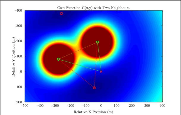
function with repulsion as negative potential and attraction as positive poten-tial; zero potential occurs at 300m. . . 55 3.7 Cost function surface in vehicle’s local reference frame, with two neighbour

vehicles, one at (−280, −81) and the other at (−25, −193); Two minima are apparent, and the closer one (at (−45, 106)) is chosen as the target point of the vehicle; this target point results in the vehicle being at the desired separation distance of 300m from both its neighbours. . . 58 3.8 Illustration of formation ’fracturing’ - grey triangles indicate a vehicle’s

neigh-bour selection triangle; here the 3 vehicles on the right have selected their two neighbours only amongst themselves, and similarly, the 8 left side vehicles have selected their two neighbours amongst themselves, resulting in the 3 vehicles drifting away from the majority. . . 59

(10)

List of Figures

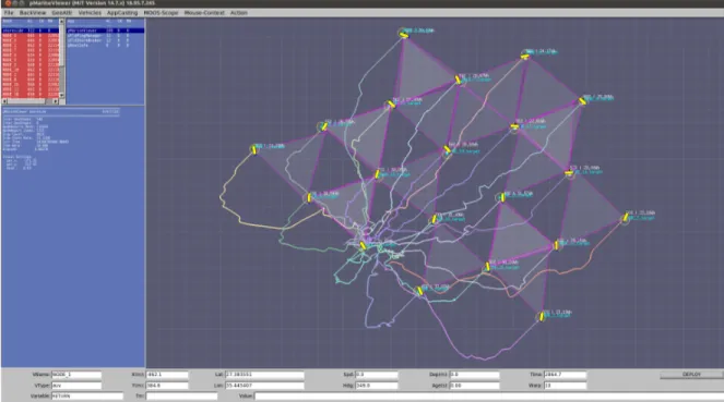
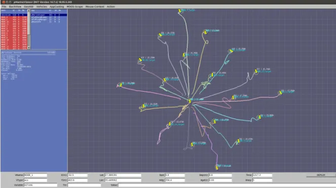
3.9 BHV AttractionRepulsion running on a swarm of 20 AUVs in the MOOS-IvP Simulation Test-Bed. . . 61 3.10 Illustration of the geometric principles behind BHV PairwiseNeighbourReferencing

running on AUV 1 for a single neighbour pair (AUV 2, AUV 3). . . 63 3.11 Illustration of the geometric principles behind BHV PairwiseNeighbourReferencing

running on AUV 1 for three neighbour pairs (AUV 2, AUV 3), (AUV 3, AUV 4) and (AUV 2, AUV 4). . . 63 3.12 BHV PairwiseNeighbourReferencing running on a swarm of 22 AUVs in the

MOOS-IvP Simulation Test-Bed (the formed letters ’NR’ are upside-down to the viewer). . . 65 3.13 Illustration of the operational principles of BHV RigidNeighbourRegistration;

for the neighbours within the vehicles CR, the corresponding points from the plan are rotated and translated to best fit the actual neighbour positions (the CR is reduced for illustrative purposes). . . 66 3.14 BHV RigidNeighbourRegistration running on a swarm of 22 AUVs in the

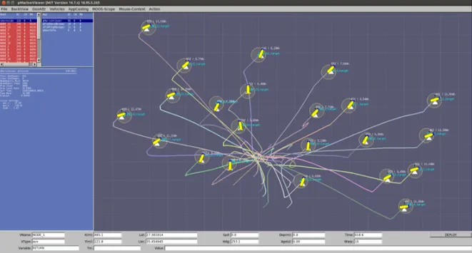
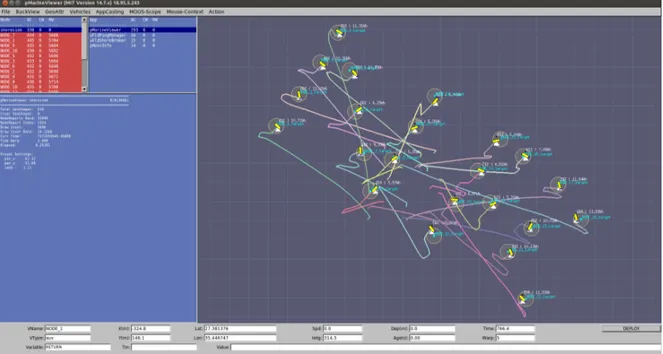
MOOS-IvP Simulation Test-Bed. . . 70 3.15 BHV AssignmentRegistration running on a swarm of 20 AUVs in the

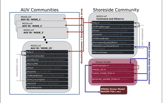
MOOS-IvP Simulation Test-Bed. . . 75 4.1 Diagram of the system architecture for the MOOS-IvP Ocean Simulation

Test-Bed; a single MOOS ’Shoreside’ community is run alongside multiple MOOS ’AUV’ communities. . . 78 4.2 Visualization in the MOOS-IvP Simulation Test-Bed of zonal and meridional

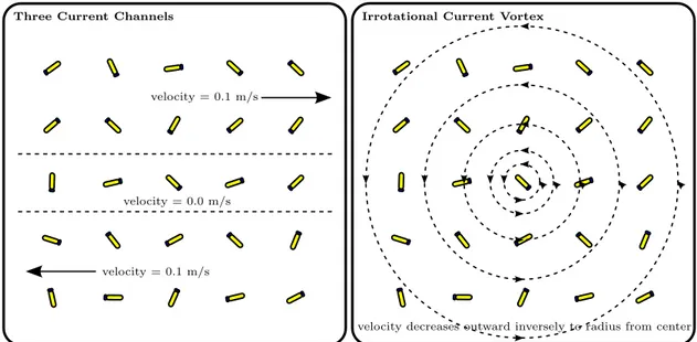
currents from an MSEAS ocean model netCDF file representing the Red Sea. . 85 4.3 Illustration of the second and third comparison scenarios - three current

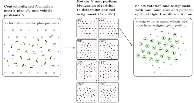
chan-nels of linear velocity, and an irrotational current vortex. . . 87 4.4 Illustration of the operational principles of the formation quality metric. . . 89 5.1 Trajectories of 25 AUVs during hexagonal lattice formation construction with

no ocean current - BHV AttractionRepulsion (trial 2); black crosses indicate starting positions, red circles indicate final positions. . . 94 5.2 Trajectories of 25 AUVs during hexagonal lattice formation construction with

no ocean current - BHV AttractionRepulsion (trial 4); black crosses indicate starting positions, red circles indicate final positions - defects are apparent in the final lattice. . . 94 5.3 Trajectories of 25 AUVs during hexagonal lattice formation construction with

no ocean current - BHV PairwiseNeighbourReferencing (trial 5); black crosses indicate starting positions, red circles indicate final positions. . . 95

(11)

List of Figures

5.4 Zoomed-in view of the trajectories of 25 AUVs during hexagonal lattice forma-tion construcforma-tion with no ocean current - BHV PairwiseNeighbourReferencing (trial 5). . . 95 5.5 Trajectories of 25 AUVs during hexagonal lattice formation construction with

no ocean current - BHV RigidNeighbourRegistration (trial 4); black crosses indicate starting positions, red circles indicate final positions. . . 96 5.6 Zoomed-in view of the trajectories of 25 AUVs during hexagonal lattice

for-mation construction with no ocean current - BHV RigidNeighbourRegistration (trial 4). . . 96 5.7 Trajectories of 20 AUVs during hexagonal lattice formation construction with

no ocean current - BHV AssignmentRegistration (trial 5); black crosses indicate starting positions, red circles indicate final positions. . . 97 5.8 Zoomed-in view of the trajectories of 20 AUVs during hexagonal lattice

forma-tion construcforma-tion with no ocean current - BHV AssignmentRegistraforma-tion (trial 5). . . 97 5.9 Trajectories of 20 AUVs during square lattice formation construction with no

ocean current - BHV PairwiseNeighbourReferencing (trial 1); black crosses in-dicate starting positions, red circles inin-dicate final positions. . . 98 5.10 Trajectories of 20 AUVs during square lattice formation construction with no

ocean current - BHV RigidNeighbourRegistration (trial 1); black crosses indi-cate starting positions, red circles indiindi-cate final positions. . . 98 5.11 Trajectories of 20 AUVs during square lattice formation construction with no

ocean current - BHV AssignmentRegistration (trial 1); black crosses indicate starting positions, red circles indicate final positions. . . 99 5.12 Trial-averaged mean energy expenditure over all AUVs during hexagonal lattice

formation construction for each behaviour with no ocean current; solid lines in-dicate trial-averaged mean energy expenditure, dashed lines inin-dicate minimum and maximum envelopes of mean energy expenditure from all trials. . . 101 5.13 Trial-averaged formation quality metric during hexagonal lattice formation

con-struction for each behaviour with no ocean current; solid lines indicate trial-averaged formation quality metric, dashed lines indicate minimum and maxi-mum envelopes of formation quality metric from all trials. . . 101 5.14 Trial-averaged mean energy expenditure over all AUVs during square lattice

formation construction for each behaviour with no ocean current; solid lines in-dicate trial-averaged mean energy expenditure, dashed lines inin-dicate minimum and maximum envelopes of mean energy expenditure from all trials. . . 102

(12)

List of Figures

5.15 Trial-averaged formation quality metric during square lattice formation con-struction for each behaviour with no ocean current; solid lines indicate trial-averaged formation quality metric, dashed lines indicate minimum and maxi-mum envelopes of formation quality metric from all trials. . . 102 5.16 BHV AttractionRepulsion - mean energy expenditure over all AUVs during

hexagonal lattice formation construction with no ocean current and varying comms. rate. . . 104 5.17 BHV AttractionRepulsion - formation quality metric during hexagonal lattice

formation construction with no ocean current and varying communications rate.104 5.18 BHV PairwiseNeighbourReferencing - mean energy expenditure over all AUVs

during hexagonal lattice formation construction with no ocean current and varying communications rate. . . 105 5.19 BHV PairwiseNeighbourReferencing - formation quality metric during

hexag-onal lattice formation construction with no ocean current and varying commu-nications rate. . . 105 5.20 BHV RigidNeighbourRegistration - mean energy expenditure over all AUVs

during hexagonal lattice formation construction with no ocean current and varying communications rate. . . 106 5.21 BHV RigidNeighbourRegistration - formation quality metric during hexagonal

lattice formation construction with no ocean current and varying communica-tions rate. . . 106 5.22 BHV AssignmentRegistration - mean energy expenditure over all AUVs during

hexagonal lattice formation construction with no ocean current and varying communications rate. . . 107 5.23 BHV AssignmentRegistration - formation quality metric during hexagonal

lat-tice formation construction with no ocean current and varying communications rate. . . 107 5.24 Mean energy expenditure over all AUVs during hexagonal lattice formation

construction with no ocean current and with node loss. . . 110 5.25 Formation quality metric during hexagonal lattice formation construction with

no ocean current and with node loss. . . 110 5.26 Trajectories of 25 AUVs during hexagonal lattice formation maintenance in

three current channels - BHV AttractionRepulsion (trial 2); black crosses indi-cate starting positions, red circles indiindi-cate final positions. . . 112 5.27 Trajectories of 25 AUVs during hexagonal lattice formation maintenance in

three current channels - BHV PairwiseNeighbourReferencing (trial 2); black crosses indicate starting positions, red circles indicate final positions. . . 112

(13)

List of Figures

5.28 Trajectories of 20 AUVs during square lattice formation maintenance in three current channels - BHV RigidNeighbourRegistration (trial 1); black crosses indicate starting positions, red circles indicate final positions. . . 113 5.29 Trajectories of 20 AUVs during square lattice formation maintenance in three

current channels - BHV AssignmentRegistration (trial 2); black crosses indicate starting positions, red circles indicate final positions. . . 113 5.30 Mean energy expenditure over all AUVs while maintaining a hexagonal lattice

formation in three current channels; two trials performed for each behaviour. . 115 5.31 Formation quality metric while maintaining a hexagonal lattice formation in

three current channels; two trials performed for each behaviour. . . 116 5.32 Mean energy expenditure over all AUVs while maintaining a square lattice

formation in three current channels; two trials performed for three behaviours. 116 5.33 Formation quality metric while maintaining a square lattice formation in three

current channels; two trials performed for three behaviours. . . 117 5.34 BHV AttractionRepulsion - mean energy expenditure over all AUVs while

maintaining a hexagonal lattice formation in three current channels and varying comms. rate. . . 118 5.35 BHV AttractionRepulsion - formation quality metric while maintaining a

hexag-onal lattice formation in three current channels and with varying communica-tions rate. . . 118 5.36 BHV PairwiseNeighbourReferencing - mean energy expenditure over all AUVs

while maintaining a hexagonal lattice formation in three current channels and with varying communications rate. . . 119 5.37 BHV PairwiseNeighbourReferencing - formation quality metric while

maintain-ing a hexagonal lattice formation in three current channels and with varymaintain-ing communications rate. . . 119 5.38 BHV RigidNeighbourRegistration - mean energy expenditure over all AUVs

while maintaining a hexagonal lattice formation in three current channels and with varying communications rate. . . 120 5.39 BHV RigidNeighbourRegistration - formation quality metric while

maintain-ing a hexagonal lattice formation in three current channels and with varymaintain-ing communications rate. . . 120 5.40 BHV AssignmentRegistration - mean energy expenditure over all AUVs while

maintaining a hexagonal lattice formation in three current channels and with varying communications rate. . . 121 5.41 BHV AssignmentRegistration - formation quality metric while maintaining a

hexagonal lattice formation in three current channels and with varying com-munications rate. . . 121

(14)

List of Figures

5.42 Mean energy expenditure over all AUVs while maintaining a hexagonal lattice formation in three current channels and with node loss. . . 123 5.43 Formation quality metric while maintaining a hexagonal lattice formation in

three current channels and with node loss. . . 124 5.44 Trajectories of 25 AUVs during hexagonal lattice formation maintenance in an

irrotational current vortex - BHV AttractionRepulsion (trial 2); black crosses indicate starting positions, red circles indicate final positions. . . 125 5.45 Trajectories of 25 AUVs during hexagonal lattice formation maintenance in

an irrotational current vortex - BHV PairwiseNeighbourReferencing (trial 1); black crosses indicate starting positions, red circles indicate final positions. . . 126 5.46 Trajectories of 20 AUVs during square lattice formation maintenance in an

irrotational current vortex - BHV RigidNeighbourRegistration (trial 2); black crosses indicate starting positions, red circles indicate final positions. . . 126 5.47 Trajectories of 20 AUVs during square lattice formation maintenance in an

ir-rotational current vortex - BHV AssignmentRegistration (trial 2); black crosses indicate starting positions, red circles indicate final positions. . . 127 5.48 Mean energy expenditure over all AUVs while maintaining a hexagonal

lat-tice formation in an irrotational current vortex; two trials performed for each behaviour. . . 129 5.49 Formation quality metric while maintaining a hexagonal lattice formation in

an irrotational current vortex; two trials performed for each behaviour. . . 129 5.50 Mean energy expenditure over all AUVs while maintaining a square lattice

formation in an irrotational current vortex; two trials performed for three be-haviours. . . 130 5.51 Formation quality metric while maintaining a square lattice formation in an

irrotational current vortex; two trials performed for three behaviours. . . 130 5.52 BHV AttractionRepulsion - mean energy expenditure over all AUVs while

maintaining hexagonal lattice formation in an irrotational current vortex and with varying communications rate. . . 131 5.53 BHV AttractionRepulsion - formation quality metric while maintaining

hexag-onal lattice formation in an irrotatihexag-onal current vortex and with varying com-munications rate. . . 132 5.54 BHV PairwiseNeighbourReferencing - mean energy expenditure over all AUVs

while maintaining hexagonal lattice formation in an irrotational current vortex and with varying communications rate. . . 132 5.55 BHV PairwiseNeighbourReferencing - formation quality metric while

maintain-ing hexagonal lattice formation in an irrotational current vortex and with vary-ing communications rate. . . 133

(15)

List of Figures

5.56 BHV RigidNeighbourRegistration - mean energy expenditure over all AUVs while maintaining hexagonal lattice formation in an irrotational current vortex and with varying communications rate. . . 133 5.57 BHV RigidNeighbourRegistration - formation quality metric while maintaining

hexagonal lattice formation in an irrotational current vortex and with varying communications rate. . . 134 5.58 BHV AssignmentRegistration - mean energy expenditure over all AUVs while

maintaining hexagonal lattice formation in an irrotational current vortex and with varying communications rate. . . 134 5.59 BHV AssignmentRegistration - formation quality metric while maintaining

hexag-onal lattice formation in an irrotatihexag-onal current vortex and with varying com-munications rate. . . 135 5.60 Mean energy expenditure over all AUVs while maintaining hexagonal lattice

formation in an irrotational current vortex and with node loss. . . 136 5.61 Formation quality metric while maintaining hexagonal lattice formation in an

irrotational current vortex and with node loss. . . 137 5.62 Trajectories of 20 AUVs during hexagonal lattice formation construction and

maintenance in the simulated Red Sea - BHV AttractionRepulsion (trial 2); black crosses indicate starting positions, red circles indicate final positions; dashed black line indicates the trajectory of the formation centroid. . . 138 5.63 Trajectories of 20 AUVs during hexagonal lattice formation construction and

maintenance in the simulated Red Sea - BHV PairwiseNeighbourReferencing (trial 1); black crosses indicate starting positions, red circles indicate final po-sitions; dashed black line indicates the trajectory of the formation centroid. . . 139 5.64 Trajectories of 20 AUVs during square lattice formation construction and

main-tenance in the simulated Red Sea - BHV RigidNeighbourRegistration (trial 2); black crosses indicate starting positions, red circles indicate final positions; dashed black line indicates the trajectory of the formation centroid. . . 140 5.65 Trajectories of 20 AUVs during square lattice formation construction and

main-tenance in the simulated Red Sea - BHV AssignmentRegistration (trial 2); black crosses indicate starting positions, red circles indicate final positions; dashed black line indicates the trajectory of the formation centroid. . . 141 5.66 Mean energy expenditure over all AUVs while constructing and maintaining

a hexagonal lattice formation in simulated Red Sea ocean currents; two trials performed for each behaviour. . . 144 5.67 Formation quality metric while constructing and maintaining a hexagonal

lat-tice formation in simulated Red Sea ocean currents; two trials performed for each behaviour. . . 144

(16)

List of Figures

5.68 Mean energy expenditure over all AUVs while constructing and maintaining a square lattice formation in simulated Red Sea ocean currents; two trials performed for each behaviour. . . 145 5.69 Formation quality metric while constructing and maintaining a square lattice

formation in simulated Red Sea ocean currents; two trials performed for each behaviour. . . 145 5.70 Mean energy expenditure over all AUVs while constructing and maintaining

a hexagonal lattice formation in simulated Red Sea ocean currents; energy expenditure detail, where dashed lines indicate the minimum and maximum envelopes of energy expenditure over all AUVs. . . 147 5.71 Mean energy expenditure over all AUVs while constructing and maintaining a

square lattice formation in simulated Red Sea ocean currents; energy expendi-ture detail, where dashed lines indicate the minimum and maximum envelopes of energy expenditure over all AUVs. . . 147 5.72 Swarm centroid travel distance divided by mean energy expenditure over all

AUVs while constructing and maintaining a hexagonal lattice formation in simulated Red Sea ocean currents; two trials performed for each behaviour. . . 149 5.73 Mean energy expenditure over all AUVs versus swarm centroid travel distance

while constructing and maintaining a hexagonal lattice formation in simulated Red Sea ocean currents; two trials performed for each behaviour. . . 149 5.74 Swarm centroid travel distance divided by mean energy expenditure over all

AUVs while constructing and maintaining a square lattice formation in simu-lated Red Sea ocean currents; two trials performed for each behaviour. . . 150 5.75 Mean energy expenditure over all AUVs versus swarm centroid travel distance

while constructing and maintaining a square lattice formation in simulated Red Sea ocean currents; two trials performed for each behaviour. . . 150 5.76 BHV PairwiseNeighbourReferencing - ratio of time spent thrusting averaged

over all AUVs to total mission time in the Red Sea scenario; dashed lines indicate minimum and maximum envelopes of this ratio over all AUVs. . . 152 5.77 BHV PairwiseNeighbourReferencing - ratio of distance travelled while

thrust-ing averaged over all AUVs to total distance travelled averaged over all AUVs in the Red Sea scenario; dashed lines indicate minimum and maximum envelopes of this ratio over all AUVs. . . 152 5.78 BHV RigidNeighbourRegistration - ratio of time spent thrusting averaged over

all AUVs to total mission time in the Red Sea scenario; dashed lines indicate minimum and maximum envelopes of this ratio over all AUVs. . . 153

(17)

List of Figures

5.79 BHV RigidNeighbourRegistration - ratio of distance travelled while thrusting averaged over all AUVs to total distance travelled averaged over all AUVs in the Red Sea scenario; dashed lines indicate minimum and maximum envelopes of this ratio over all AUVs. . . 153 5.80 BHV AssignmentRegistration - ratio of time spent thrusting averaged over all

AUVs to total mission time in the Red Sea scenario; dashed lines indicate minimum and maximum envelopes of this ratio over all AUVs. . . 154 5.81 BHV AssignmentRegistration - ratio of distance travelled while thrusting

av-eraged over all AUVs to total distance travelled avav-eraged over all AUVs in the Red Sea scenario; dashed lines indicate minimum and maximum envelopes of this ratio over all AUVs. . . 154

(18)

(19)

List of Tables

3.1 Parameters of the DriftingTarget behaviour. . . 49

3.2 Parameters of the ManageAcousticPing behaviour. . . 53

3.3 Parameters of the AcousticPingPlanner behaviour. . . 53

3.4 Important parameters of the BHV AttractionRepulsion behaviour. . . 55

3.5 Important parameters of the BHV PairwiseNeighbourReferencing behaviour. . 62

3.6 Important parameters of the BHV RigidNeighbourRegistration behaviour. . . . 66

3.7 Important parameters of the BHV AssignmentRegistration behaviour. . . 74

4.1 Important configuration parameters of the uSimConsumption MOOSApp. . . . 82

4.2 Important configuration parameters of the iMSEASOceanModelDirect MOOS-App. . . 84 4.3 Important configuration parameters of the pFormationQualityMetric MOOSApp. 89

(20)

(21)

Chapter 1

Introduction

The past decade has seen rapid progress in autonomous underwater vehicle (AUV) technol-ogy, with a growing interest and adoption of such vehicles for scientific, commercial, and defence applications in the underwater domain. These vehicles have the potential to fun-damentally impact data gathering approaches in these fields. In addition, the emergence of swarm robotics research during this decade, where the concepts of swarm intelligence are applied to multi-robot systems, is allowing scientists and other users of robotics systems to leverage the use of multiple coordinated robots in achieving desired goals. As AUV technol-ogy continues to mature, the development of distributed cooperative and swarm autonomy for AUVs can potentially address issues more effectively than a single AUV typically can; for example, monitoring and determining the location of toxic ocean spills, tracking algae or phytoplankton blooms or other oceanographic chemical and biological phenomena, or the use of a swarm as a virtual sensor array for seismic surveying. A swarm of AUVs using ocean currents for propulsion has several attractive characteristics for undersea monitoring; such a swarm would be able to exploit ocean currents to monitor ocean phenomena for long periods of time while contributing very little ambient noise; the characteristics of the swarm would contribute to its endurance by being fault tolerant, as well as allowing it to flexibly survey areas of complex geometry containing obstacles; and the swarm would be able to monitor areas of large expanse, enabling effective investigation of the structure of complicated ocean phenomena. In addition, the characteristics of the underwater environment necessarily force unique constraints on the swarm robotics problem (namely in terms of communication and localization), and the development of autonomous behaviours that can successfully overcome these constraints has the potential to contribute greatly to the field of swarm robotics.

Recognizing the potential advantages of the use of a large, coordinated group of AUVs for oceanographic data gathering, the principal objective of this work is to investigate approaches to swarm navigation and formation control in the underwater realm. The communications

(22)

Chapter 1. Introduction

constraints of such an environment, with data rates on the order of 100 bits per second to 5000 bits per second, and the fairly frequent loss of packets, poses significant challenges on the ability to form and maintain multi-vehicle AUV formations. Although the existing liter-ature on multi-robot formation control is sizeable, the unique constraints of the underwater domain implies that it is not simply a matter of applying existing above-ground techniques to the underwater realm - its constraints necessitate the development and testing of formation control behaviours that can operate successfully with significant restrictions on inter-vehicle communications. An investigation into this issue is the main contribution of this thesis.

1.1 Contributions

This thesis presents three contributions - the primary contribution is the development of four different formation control behaviours which are implemented in the MOOS-IvP autonomy infrastructure, and which allow a group of AUVs to form lattice or pattern formations that are rotationally and translationally invariant. The second is the proposal of a formation quality metric. This metric quantifies how well the behaviour is able to maintain the desired swarm formation, and is used in conjunction with formation energy expenditure (how efficiently the behaviour uses energy to maintain formation), and formation robustness (how well the formation is maintained in the presence of node failure and varying communication rate), to compare the efficacy of each behaviour. Finally, the current MOOS-IvP AUV simulation test-bed is augmented to allow the accurate simulation of ocean currents, as well as acoustic communication between multiple vehicles.

1.1.1 Lattice/Pattern Formation Behaviours in MOOS-IvP

The formation of lattices or patterns by a swarm of autonomous underwater vehicles is the principal objective of this work. We envision the use of such a formation of AUVs for two specific applications - by equipping each vehicle with an acoustic receiver, the formation can be employed as a ’virtual’ acoustic array, allowing its use as the receiver for sea-bottom seis-mic surveying, or the monitoring of naturally occurring acoustic and seisseis-mic radiation from ice; secondly, by equipping each vehicle with biological sensors, biological phenomena which are very spatially and temporally dynamic (such as phytoplankton blooms) can be moni-tored with greater accuracy over large regions. Ideally, behaviours would allow the swarm to autonomously maintain a formation without requiring a comprehensive navigation and communication infrastructure, using a paradigm similar to that of a school of fish, where each vehicle navigates and maintains formation solely by communicating acoustically with its nearest neighbours. In addition, we wish to maximize the length of such missions, explicitly by making use of ocean currents as a means of propelling the swarm formation. In order to

(23)

increase the endurance of missions using the swarm, the swarm is expected to utilize average ocean currents for propulsion, with the vehicles using their motors only as a means of main-taining formation geometry. Finally, given the communications constraints of the underwater environment, pattern formation cannot be performed in a centralized (or even decentralized) manner - all behaviours must be completely distributed.

Taking into account these ambitions, as well as the constraints of the underwater environ-ment, four pattern formation behaviours were developed in an attempt to meet these goals and challenges. A brief overview of each is provided here.

Attraction/Repulsion Atomic Model (BHV AttractionRepulsion)

I present a lattice formation behaviour based on the idea of interatomic forces. As the forces between atoms naturally produce a hexagonal lattice, applying similar forces between vehicles is an obvious method for producing a hexagonal lattice formation of AUVs. This idea has been well researched in past swarm robotics literature, under the broad title of physics-based formation control, but my implementation uses a direct optimization technique to determine the force minimum, a novel extension of past work.

Pairwise Neighbour Referencing (BHV PairwiseNeighbourReferencing)

This approach requires a predetermined plan of the formation pattern, as well as communi-cation of unique vehicle IDs. The plan details the shape and scale of the formation, with the relative positions of each vehicle within the formation. Every vehicle utilizes this plan in order to reference itself against pairs of its neighbours, using the angle and distance between itself and each pair to determine its relative optimal location. This is perhaps one of the simplest approaches to pattern formation, but is robust, translationally and rotationally invariant, allows any arbitrary shape to be formed, and as far as I can tell, has not been described in previous literature.

Rigid Neighbour Registration (BHV RigidNeighbourRegistration)

This behaviour was inspired in part by the iterative closest point (ICP) algorithm and as an approach to improving on the previous behaviour. ICP is widely used to align two point clouds without knowing the correspondence between individual points in each cloud; however, if the correspondences are user defined, the alignment between the clouds, in which we wish to minimize the mean-squared error in distance between all points (by selecting an optimal rotation and translation combination), has a closed-form solution. This error minimization problem is known as the orthogonal Procrustes, or the rigid point set registration problem, and is the transformation step in the ICP algorithm. In terms of pattern/lattice formation,

(24)

given our predetermined plan and unique vehicle IDs that correspond to positions in our plan, this behaviour transforms the plan to the actual vehicle positions in a distributed manner, so as to create the desired pattern.

Assignment Registration (BHV AssignmentRegistration)

In an attempt to improve on the Rigid Neighbour Registration behaviour, I present a novel approach that attempts to both perform the point correspondence between the plan and vehicles, and the rigid point set registration. Vehicles are assigned to points in the plan dynamically via the Hungarian algorithm so as to minimize distance travelled, and as before, minimization of the mean-squared error in distance is used to determine the optimal rotation and translation of the local plan. By removing the requirement of unique vehicle IDs, I hope to reduce the communication requirement between vehicles.

1.1.2 Formation Comparison Metrics

A goal of this work is to compare the efficacy of each behaviour, with respect to our scenario - we wish to form a lattice formation with minimal energy expenditure by each vehicle in the swarm, and once formed, we want the formation to maintain its shape, utilizing surface currents as effectively as possible for swarm travel (expending energy only to maintain shape). To perform this comparison, I developed a metric to quantify the quality of the formation, using a similar approach used in the Assignment Registration behaviour above. Given the location of each vehicle, and the lattice formation we wish to achieve, I essentially assign each vehicle to a point in the desired formation so as to minimize Euclidean distance using the Hungarian algorithm, and then determine the optimal rotation and translation of the desired formation to minimize the mean-squared error between each point. The value of this error is used as the quality comparison metric.

This metric is used as a comparison against energy expenditure (both during the forming of the formation, and during the maintaining of the formation), as well as against vehicle failure and communication rate to determine formation robustness.

1.1.3 Comparison Scenarios, Behaviour Testing, and the MOOS-IvP Ocean Simulation Test-Bed

Each behaviour is tested in four comparison scenarios, where each scenario represents a dif-ferent ocean current field - the first is a field with no currents; the second is in a field of three current channels of different velocity; the third is in a vortex current field; and the fourth is in a current field representing realistic ocean currents. These scenarios and testing of each

(25)

behaviour for comparison is performed in the MOOS-IvP Ocean Simulation test-bed.

The MOOS-IvP Ocean Simulation test-bed provides a platform to test autonomous be-haviours using accurate ocean current dynamics, acoustic communications, and vehicle dy-namics, and allows the user to visualize these behaviours in rates faster than real-time. My contribution to improving this test-bed is in the efficient integration of ocean current simu-lations provided by the MIT MSEAS group, allowing us to utilize the test-bed for scenarios with highly realistic ocean currents.

1.2 Summary

This chapter has presented the reader with an overview on the motivations, objectives, and contributions of the work undertaken in this thesis. I have described the behaviours I have implemented for the goal of forming desired lattice or pattern formations for a group of AUVs, the metrics by which I evaluate each behaviour on its ability to produce the desired formation, and the scenarios and test-bed used to undertake these comparisons.

The remainder of this thesis is organized into six chapters. Chapter 2 provides the reader with an outline of background topics pertinent to my research, as well as a survey of re-lated literature in swarm robotics. Chapter 3 provides a detailed explanation of the four lattice/pattern formation behaviours implemented for this thesis. Chapter 4 gives the reader an overview of the methodology, infrastructure, and comparison metrics used to evaluate each behaviour in simulation. Chapter 5 provides the results and an analysis of the comparison metrics. Finally, chapter 6 details a discussion of the results of the analysis, conclusions drawn from this research, and future work to be undertaken.

(26)

(27)

Chapter 2

Background and Related Work

To give the reader a good understanding of the work undertaken in this thesis, we provide a gentle introduction to background topics related to this research, with the assumption of little prior knowledge from the reader. We begin with an overview of autonomous underwater vehicles, the platform that we envision this work to be applied to; this is followed by an introduction to MOOS-IvP, the software architecture I have used to implement my work; we then provide a broad outline of swarm robotics and swarm intelligence research, with a more detailed review of prior work in swarm formation control; and finally, we specify the numerous assumptions along with the scope of this work, and summarize.

2.1 Autonomous Underwater Vehicles

Autonomous underwater vehicles (AUVs) are untethered underwater mobile robotic systems that carry a sensor payload that is typically used for measuring water properties and the ocean bathymetry and environment. In recent years, AUVs have become an increasingly valuable and popular tool for oceanographic research, and the dramatic improvement in their capabil-ities and reliability over the past two decades has resulted in a growing interest in their use for scientific, commercial, and military applications. The commercialisation of AUVs has also meant that they now potentially provide a cost effective alternative to traditional ship-based oceanographic sampling and measurement. Depending on the application, AUVs can provide a number of advantages over traditional methods. For example, with regards to scientific oceanography, ship-based methods can be limited in their sampling rate and their ability to measure highly dynamic and unpredictable spatial and temporal ocean phenomena. In con-trast, AUVs have demonstrated their utility in gathering time-series oceanographic data by repeated water column surveys, and their autonomy opens up the prospect of adaptive be-haviours that may allow the effective tracking of dynamic ocean phenomena. In the military sphere, the autonomy of AUVs potentially allows their use in areas which are restricted to,

(28)

Chapter 2. Background and Related Work

or dangerous for personnel, and their minimal profile presents their possible application in covert operations.

The majority of currently available AUVs can be classified into four categories depending on their intended application; these categories are shallow water survey AUVs, mid-water AUV’s, deep-water AUVs, and glider AUVs. Shallow water AUVs are designed to operate in coastal and littoral areas, and at depths less than 500 meters. They are typically fairly small (usually around 1-2 meters) since they do not have to withstand high water pressures, and have a high drag to thrust ratio, which allow them to manoeuvre in areas with high currents. These vehicles are typically used to survey areas fairly quickly, and at low resolution, and so their operating speeds are relatively high. Mid-water AUVs are usually rated for depths of up to 2.5 kilometres, and are typically used to perform mid-water column surveys or surveys in shallower areas. In order to handle the pressure at these depths, these vehicles are usually quite bulky, which in turn means that they need more thrust and power, adding to their size (which range from 4-6 meters in length). As the currents at these depths are generally low, AUVs in this class can have a small drag to thrust ratio. Depending on their applica-tion, their operating speed can vary from less than one knot to several knots. Deep-water AUVs are designed to be used at depths greater than 2.5 kilometres, and are typically large in volume in order to withstand the high oceanographic pressures at such depths. Since this class of AUVs are usually used close to the bottom of the ocean floor for high resolution sur-veys, they are designed to manoeuvre at low speeds. As such, their design is typically quite different to that of shallow water survey and mid-water AUVs, the majority of which have a tubular, torpedo-shaped hull and use a single propeller in conjunction with elevators and fins. In contrast, deep-water AUVs usually have multi-hull designs with multiple thrusters. Glider AUVs operate in a significantly different manner to that of the previous AUV classes, in that they are propelled through the water via changes in buoyancy and water temperature in conjunction with wings to convert vertical motion into forward motion. This propulsion method typically achieves a much higher efficiency than conventional electric thrusters, in-creasing their range to the order of thousands of kilometres, at the expense of horizontal and vertical manoeuvrability. These vehicles usually operate in the upper water column, and are typically rated for depths of less than 1 kilometre.

In more recent years, an additional class of AUVs has emerged - the long-range AUV. These AUVs have been specifically designed in order to perform sampling of oceanographic processes that evolve over periods of days or even weeks, and as such, are built with the goal of maximizing endurance. In order to do so, they are designed with novel improvements to previous AUV classes, such as active buoyancy control, allowing them to sample processes at a desired depth without expending energy on propulsion. Two such examples of these AUVs

(29)

are the Tethys [1] AUV built at MBARI, and which has active buoyancy control and utilizes custom energy saving strategies (such as power-down of motor controllers and non-essential systems), and the Folaga [2] AUV built by Graaltech, which similarly has active buoyancy control as well as an actuation mechanism that allows it to propel as a glider. We envision the use of this class of AUVs for long endurance multi AUV oceanographic sampling, and their emergence can be interpreted as an endorsement for the benefit of using swarms of AUVs for this purpose.

Despite the enormous developmental gains in autonomous underwater vehicle technology over the past few decades, there remains a number of challenges facing their applicability and usefulness. This includes challenges in power consumption, navigation and positional accuracy, underwater communications, and intelligent and adaptive autonomy. As the focus of this thesis is the investigation of autonomous swarm behaviours, the architecture that I use to develop and implement such behaviours, as well as existing examples of swarm robotics, are expanded upon here.

2.2 MOOS-IvP

MOOS-IvP [3] is an open-source software infrastructure used for the development of au-tonomous behaviours for unmanned marine vehicles. It is composed of two open-source projects - MOOS (the Mission Oriented Operating Suite), which provides core middleware capabilities in a publish-subscribe architecture, whereby MOOS applications (MOOSApps) asynchronously publish and subscribe to information from a central database (the MOOSDB); and the IvP (Interval Programming) Helm, a foundational MOOS application that provides vehicle behaviour arbitration via multi-objective optimization, deciding upon an optimal out-put (typically vehicle heading, speed and depth) by evaluating competing behaviours. The IvP portion of this infrastructure was developed by the Laboratory of Autonomous Marine Sensing Systems (LAMSS) at MIT, a group of which I am part, and consequently this is the software of choice for the implementation of my behaviours.

In the context of this work, the organization of the MOOS-IvP architecture is as fol-lows; a single centralized ’shoreside’ MOOS community is run, which houses a number of MOOSApps related to the extraction or calculation of ocean currents, the evaluation of the formation quality metric, and formation visualization; in addition, each vehicle in the swarm has its own MOOS community, running MOOSApps related to simulating vehicle dynamics, calculating energy consumption, and an IvP helm to process the formation behaviours. To simulate acoustic communication, vehicle MOOS communities pass information related to vehicle state to the shoreside MOOS community, the acoustic communication is simulated

(30)

centrally (adding noise etc.), and the result is passed back to each vehicle - anything that must be centrally computed for simulation purposes (such as ocean currents) is performed in the same way. It must be stressed, however, that behaviours described in this work are entirely distributed - the shoreside MOOS community is not used to control the behaviour of individual vehicles.

On each vehicle, the IvP helm solves for optimal control (heading, speed and depth) using:

x∗ = argmax x k−1 X i=0 wifi(x) (2.1)

where each fi(x) is an objective function produced by each active behaviour on the vehicle,

and each wi is a relative priority weighting for the behaviour. As such, the IvP helm attempts

to determine the parameters for which the sum of the objective functions for each active behaviour is maximized, and does so by evaluating the objective function of each behaviour over the entire decision space. How this is achieved is detailed in [3].

2.3 Swarm Robotics and Swarm Intelligence

Swarm robotics has emerged in the past decade as an area of research concerned with the application of swarm intelligence [4] concepts to multi-robot systems. Swarm intelligence is a form of distributed intelligence, in which the collective behavior of a group emerges out of the simple behaviors of its autonomous individuals through local peer interaction, and inter-actions with the environment. Although swarm robotics systems are not explicitly required to be distributed, research in swarm robotics is often inspired by biological systems, such as insect colonies (for example, cockroaches [5], ants [6] or bees [7]), flocks of birds [8], schools of fish [9], and bacteria colonies [10]. The absence of centralized control in such biological systems provides a number of advantages, and by seeking to replicate these advantages, many swarm robotics systems are typically distributed. This lack of centralization gives such sys-tems implicit advantages of fault tolerance (failure of any single individual has little effect on the success of the group), flexibility (self organization and no reliance on global informa-tion), and scalability (behaviors are local so that the addition or removal of individuals has little impact on swarm performance). Swarm robotics has been a growing area of research over the past two decades, especially in the land and air domains. Unfortunately, until very recently little research has been performed in the underwater domain, and the limitations of the ocean environment provide a unique variation to the regular challenges of swarm au-tonomy. Here we provide a broad overview of different facets of swarm autonomy, and look especially at previous research directed at distributed swarm formation control. This section

(31)

is by no means an exhaustive review of swarm robotics, but the interested reader is directed to [11], [12], [13], [14] and [15] for good reviews of the recent state of the art in this research area.

Swarm robotics presents researchers with a range of potential advantages over single robot systems, and these advantages are the prime motivators behind swarm research. Swarm robotics systems are envisioned to be able to:

• Exploit the sensing capabilities of large groups, allowing the efficient discovery and exploration of areas of interest, as well as improve situational awareness.

• Provide superior robustness against mission failure, since the failure of a single agent in the group can be mitigated by other agents.

• Parallelize mission tasks amongst agents in the group, allowing a mission to be completed faster than if performed by a single agent. In addition, this distribution of tasks may enable swarms to achieve greater results, such as conducting missions over larger areas, manipulating objects or the environment more efficiently, or attacking with numbers. • Be adaptable and scalable, allowing missions to continue via task reallocation with

the addition and removal of agents in the group. Since interactions are localized, the addition or removal of agents does not require any change to control software.

• Be cost effective. By using many simple vehicles, rather than a single complex vehicle, swarms are able to have a greater cost effectiveness, by virtue of the fact that a loss of one simple vehicle in the swarm has less impact than the loss of a single more powerful vehicle.

However, these advantages come together with a couple of drawbacks. Firstly, operator com-mand and control of large robotic swarms is difficult; centralized C&C schemes may not scale well with increasing number of agents, and decentralized C&C schemes may have trouble gathering and synthesizing data from all members of the swarm; deployment and retrieval of such swarms is also an open question. Secondly, because the design of behaviours of agents in the swarm is done with local interactions in mind, the global behaviour of the swarm can be difficult to predict, as it emerges from numerous locally interacting agents.

The design of robotic swarm systems include considerations that can be broadly defined into two categories - architecture and application. Within the architecture category, the de-signer must consider a number of facets that must be selected with respect to the intended application of the swarm. These include the selection of heterogeneous versus homogeneous robot swarms, centralized versus distributed control schemes, and communication structures.

(32)

Within the application category, the designer must develop specific or groups of swarm strate-gies that can most effectively address the desired task. These stratestrate-gies include swarm be-haviours such as aggregation [16], [17], dispersion [18], task allocation [19], coordinated col-lective motion [20], [21], object transportation [22], colcol-lective exploration and mapping [23], [24], and pattern formation. Within the scope of our work here, we can classify our swarm system as being homogeneous (within our application we wish to have single-type AUVs that either serve as acoustic receivers, or are able to sense a specific oceanographic phenomena), distributed (since the constraints of the underwater domain prohibit sufficient communication bandwidth for centralized control), having a local communications range (as acoustic com-munications becomes much less reliable at larger distances), and having a pattern formation behaviour (as this is what is required to achieve our desired goals). With this in mind, we limit our literature review to cover pattern formation approaches for robotic swarm systems that have a similar architecture. We do not provide an overview of differences in architecture or review approaches for applications other than formation control. As before, the interested reader is directed to [11], [12], [13], and [14] if they desire greater insight into these topics.

2.3.1 Distributed Swarm Formation Control

In swarm robotics, the term pattern formation control has been used in at least two different ways. Firstly, pattern formation has been used to broadly encompass multiple aspects of pat-terns of agents, including the establishment, maintenance and reconfiguration of patpat-terns or lattices, rather than exclusively pattern establishment. Secondly, the term pattern formation has been used in literature interchangeably with the phenomenon of swarm flocking, which de-fines behaviours that are loosely geometric in nature. In term of this work, we refer to swarm formation control in the sense of the first definition - we mean pattern or lattice formation control as behaviours that produce and control well defined geometric patterns of agents in the swarm. In the context of this definition, past research can be broadly categorised into four groups, each of which we examine here. For further reading and other reviews of swarm formation control, we direct the reader to [25] and [26].

Physics-Based Approaches

One of the most common approaches to pattern formation in swarms is the physics-based approach. In this approach, formation generation is often inspired by the physics of atoms, molecules or crystals, or by the physics of springs. Physics-based formation design use virtual forces to coordinate the movement of agents in the swarm.

One of the earliest and most well-known physics-based approaches is the ’Physicomimet-ics’ framework, introduced by Spears et al. [27], [28]. In their approach agents in a swarm

(33)

react to virtual forces inspired by natural physics laws. At an abstract level, agents are used to mimic physical structures of particles, with each particle having a position and a velocity. At each time step of the algorithm, particle positions are perturbed by an amount dependent on its current velocity; this velocity is itself modified at each time step in accordance to a force law applied to the particle by its neighbours; and this force law is essentially a repul-sion/attraction force of certain radii centred at each particle. Using this approach, they are able to form hexagonal lattices which attempt to minimize an overall ’potential energy’ of the swarm. They are also able to develop an analytical model of the potential energy wells that cause the formation of this hexagonal structure, providing an analysis of lattice quality. They also extend their work to produce square lattices, and provide strategies to prevent agents from falling into local minima. They demonstrate their Physicomimetics technique in both simulation and on a group of seven robots. In [29], Prabhu et al. extend this framework to produce stable hexagonal cells, and to remove lattice imperfections.

In [30], Pinciroli et al. present a similar approach, whereby local artificial potential fields centred around each agent are modelled after the interatomic Lennard-Jones potential model (used to approximate the interaction between neutral pairs of atoms) in order to produce a hexagonal lattice of simulated pico satellites. However, in order to induce aggregation in the agents, they introduce a global potential field centred at a desired coordinate, so as to draw all agents to a single point. For stabilization, they also include a third damping term to prevent oscillations commonly observed in physics-based approaches.

Similarly, Gazi and Passino [31] introduce different classes of attraction/repulsion artifi-cial potential functions for distributed formation control. Their artifiartifi-cial potential functions include linear attraction/bounded repulsion, linear attraction/unbounded repulsion, and con-stant attraction/unbounded repulsion, each of which they analyse in the context of swarm cohesion, and provide simulation results.

An alternative approach to attraction/repulsion schemes is the artificial springs technique, first introduced by Fujibayashi et al. [32], where potentials are modelled as artificial springs with varying coefficients. In this work, each agent generates virtual springs between itself and neighbouring agents, based on the number of its neighbours within a specified radius, in order to produce a crystalline lattice structure. To produce a desired lattice, they modify the spring constant and natural length properties of each spring depending on the number of connections of the agents on either end of the spring; they also include a method of separating agents. By introducing certain combinations of springs and through tuning they are able to generate desired shapes.

(34)

Shucker and Bennett [33] present a similar approach, using a virtual spring mesh to con-trol a formation of robots. In this work, the authors describe an algorithm that concon-trols the creation and destruction of virtual springs between agents that operates in the following way -a robot R will cre-ate -a spring with its neighbour S, if for every other neighbour T, the interior angle RTS is acute. They argue that such an approach will influence the swarm to create a hexagonal lattice, because such a lattice is the only optimal zero-energy state of the system. They provide simulation examples for swarm exploration and target tracking, and analyse the system in the case of catastrophic agent failures.

Finally, Stolkin and Nickerson [34] provide a review and comparison of different physics-based approaches, and propose a novel method that combines them - they use an attrac-tion/repulsion model to form local clusters of agents, then use a spring technique to group clusters together. This allows local clusters to produce regular lattices, while attracting local clusters together quickly via spring-like attraction behaviours. Unfortunately this method is decentralized; it is not completely distributed.

Potential Field Approaches

Potential Field approaches to swarm formation are somewhat similar to physics-based ap-proaches, but differ in one important way - the potential field is global, rather than local. In these approaches, this global potential field is used to actuate agents toward minima in the desired shape of the formation.

Perhaps one of the earliest use of this approach is presented by Bachmayer and Leonard in [35]. In this work, they use artificial local potentials to maintain group geometry, while at the same time using a gradient descent method to drive the group toward a minimum. They achieve this by having each agent sum an approximation of the world gradient with the local potentials of its neighbours; the world gradient is approximated using a single sensor which is assumed to be able to measure the gradient only in the direction of agent motion. Al-though usually such an approach would cause an agent to find a minimum only along a ’slice’ of the world, the introduction of inter-vehicle potential functions enables the group to com-municate enough information to determine the global world minimum in an emergent manner.

Chaimowicz et al. [36] present an approach to swarm formation whereby they create po-tential fields whose minimum lies along a 2D curve described by an implicit function. This implicit function is viewed as the zero isocontour of the 3D potential field, whose value is greater than zero outside the isocontour, and less than zero inside the isocontour. By making each agent perform a gradient descent on the potential field (and inverting the gradient when

(35)

the agent is within the isocontour), the authors are able to direct the agents to converge along the desired isocontour. They are able to produce a wide variety of desired formation shapes, including letters, using this implicit function approach. The authors provide an analysis of system performance, as well as results from simulations of tens of robots and experimental results with a team of six vehicles.

In her PhD dissertation, Barnes [37] demonstrates the results from a similar approach -artificial potential fields are generated using normal and sigmoid functions, as well as other limiting functions, to control overall swarm geometry and spacing. She presents the results from simulations of four to ten vehicles performing circle, wedge and ellipse formations. Using a fuzzy speed controller, she directly uses the gradient of the potential field to direct the movement of agents in the swarm.

Virtual Structure Approaches

The virtual structure approach was first introduced by Lewis and Tan [38]. In this approach a rigid formation (referred to as a structure) is defined, within which agents maintain a rigid geometrical relationship. In this way, the entire swarm is treated as a single rigid body, with agents acting as vertices of the body.

In the approach originally presented by Lewis and Tan [38], the authors present an algo-rithm which is composed of four steps - the first step involves aligning the virtual structure to the current positions of agents in the swarm, via an optimization problem to minimize the difference between actual and desired agent positions; the second step displaces the virtual structure toward a desired mission objective; the third involves computing agent trajectories so as to realign their positions with the structure within a specified time window; and the final step directs the agents to follow the calculated trajectories. Unfortunately, their original approach was centralized; however, Ren and Beard [39] present a decentralized extension to this work using local controllers.

Belta and Kumar present a control approach [40] that designs trajectories such that a rigid formation of agents will maintain their geometry. Specifically, the method outlined generates trajectories that minimizes the total energy associated with the translations and rotations of the robots, while maintaining their current formation. Their method involves three steps; the first generates optimal trajectories for the formation; the second projects these trajectories on a specified Euclidean group that represents the gross position and orientation of the swarm, the set of shape variables that describe the relative positions of robots in the swarm, and the control graph that describes each robot’s control strategy; the third step performs a

(36)

tion of the motion to position trajectory for each individual robot.

In [41], Egerstedt and Hu present a model-independent coordination strategy for swarm formations, where instead of designing control laws for the agents directly, they assume agents possess existing tracking controllers and instead design an algorithm that generates reference points. The desired formation structure is defined relative to a virtual formation leader, and this leader moves along a parametrized path. The trajectory of each agent is selected so as to propagate in the direction that minimizes a specified control function, where the magnitude of the motion depends on how well the agent tracks the structure. In turn, the velocity of the virtual leader along the path is dependent on the tracking errors of all the agents.

Leader-Follower Approaches

In leader-follower approaches, a hierarchy of agents is defined within the formation, meaning that such approaches inherently require the communication of unique agent IDs. Followers attempt to maintain formation with their respective leader(s), whose motions are either pre-scribed (such as following a specified path) or who themselves follow their own leader(s). In addition, leaders do not necessarily have to be physical agents in the swarm, as virtual leaders can also be used to effectively control group motion.

Desai et al. [42] presents a popular leader-follower control strategy whereby feedback linearisation is used, along with a formation plan defined by relative angles and distances between agents to produce two feedback controllers - the first is a separation/bearing con-troller between a follower and its leader, and the second is separation/separation concon-troller between a follower and two leaders. Other authors expand upon this approach with other control strategies, such as dynamic feedback linearisation [43], model predictive control [44], [45], and first and second order sliding mode control [46].

In [47], Elkaim and Kelbley combine a leader-follower approach with a physics-based approach. They describe a formation whose geometric structure is maintained via inter-vehicle artificial forces, and which travels along a desired trajectory using artificial forces between each vehicle and a virtual leader which is guided along the trajectory. The general methodology of this approach is as follows - first, all of the forces that are acting upon the agents are calculated; secondly, the point at which the sum of these forces is zero is determined; finally this point is then used as the reference position for each individual vehicle, which moves towards the point using its own kinematic controller. This process is iteratively repeated.

(37)

Other Approaches

Besides the approaches categorized in the sections above, a considerable amount of research in swarm formation control does not fit comfortably in the physics-based, potential field, virtual structure or leader-follower groups. We examine some here.

In [48] Song and O’Kane present a novel decentralized algorithm for forming arbitrary multi-robot lattices, such as squares, hexagons, and octagon-squares. Their approach makes use of an author-defined ’lattice graph’ (not to be confused with lattice graphs of graph the-ory). This lattice graph is a strongly connected directed multigraph whose edges describe a rigid-body transformation, and is used to define the desired lattice of the swarm. Their al-gorithm requires the broadcast of short messages between neighbouring agents, and executes the following series of four steps. First, each agent must decide whether to consider itself as a root robot (one that remains motionless), or a descendant robot (one that moves in accor-dance to a task assignment from a parent); this decision is made based on an author-defined ’authority’, which depends on robot ID as well as information about robot’s ’ancestors’, and is done to ensure that agents form a stable forest of authority trees. Secondly, agents select a role; root agents always select the first lattice vertex as their role, and descendant agents accept their role by task assignment from their parent. Thirdly, after role selection, each agent computes a locally optimal task assignment for its neighbours, using the Hungarian algorithm; each agent broadcasts this assignment and their authority value to its neighbours. In the final step, each descendant agent moves toward the position assigned by its parent, while staying within communication range. The authors present the results of their algorithm using a simulation of between 50 and 250 robots.

Lee and Chong [49] demonstrate a distributed algorithm for lattice formation using sim-ple geometric princisim-ples. In their approach, an agent selects two of its neighbours such that the triangular path travelled by the positions of three agents is minimized; then using these two neighbouring agents, the robot calculates the centroid of the triangle formed by itself and its neighbours, and measures the angle between the line connecting two neighbours and its horizontal axis; finally, in reference to the calculated centroid and using this angle and a desired inter-agent separation distance, the robot repositions itself to a target that is com-puted using simple trigonometric equations such that it forms an isosceles triangle with its two neighbours. The authors prove convergence of this algorithm using Lyapunov stability theory, and demonstrate formation self-repair in simulations of 100 robots.

Lee and Chong [50] also present another approach using similar geometric principles, but in which agents are referenced against neighbours and a local leader is dynamically selected.