HAL Id: hal-03187627
https://hal.archives-ouvertes.fr/hal-03187627
Submitted on 1 Apr 2021
HAL is a multi-disciplinary open access
archive for the deposit and dissemination of
sci-entific research documents, whether they are
pub-lished or not. The documents may come from
teaching and research institutions in France or
L’archive ouverte pluridisciplinaire HAL, est
destinée au dépôt et à la diffusion de documents
scientifiques de niveau recherche, publiés ou non,
émanant des établissements d’enseignement et de
recherche français ou étrangers, des laboratoires
Grounding, Quantifiers, and Paradoxes
Francesco Genco, Francesca Poggiolesi, Lorenzo Rossi
To cite this version:
Francesco Genco, Francesca Poggiolesi, Lorenzo Rossi. Grounding, Quantifiers, and Paradoxes.
Jour-nal of Philosophical Logic, Springer Verlag, In press. �hal-03187627�
Grounding, Quantifiers, and Paradoxes
∗
Francesco A. Genco
[email protected]
Francesca Poggiolesi
[email protected]
Lorenzo Rossi
[email protected]
AbstractThe notion of grounding is usually conceived as an objective and ex-planatory relation. It connects two relata if one—the ground—determines or explains the other—the consequence. In the contemporary literature on grounding, much effort has been devoted to logically characterize the formal aspects of grounding, but a major hard problem remains: defin-ing suitable grounddefin-ing principles for universal and existential formulae. Indeed, several grounding principles for quantified formulae have been proposed, but all of them are exposed to reflexivity and symmetry para-doxes in some very natural contexts of application. We introduce in this paper a first-order formal system that captures the notion of grounding and avoids, in a novel and non-trivial way, both reflexivity and symme-try paradoxes. The presented system formally develops Bolzano’s ideas on grounding by employing Hilbert’s ε-terms and an adapted version of Fine’s theory of arbitrary objects.
Keywords: grounding; quantifiers; epsilon calculus; arbitrary objects; Bolzano.
1
Introduction
The notion of grounding has recently received increasing attention in different areas of philosophy: from explanation, to metaphysical dependence and funda-mentality, to the analysis of logico-linguistic operators [3, 28, 32, 14, 8, 30, 7, 25, 26, 33, 21, 22]. Grounding is usually conceived as an objective and explana-tory relation. It connects two relata if one—the ground—determines or explains the other—the consequence. Hence, the ground constitutes a reason why the consequence holds; the consequence, in turn, holds in virtue of the ground.
A branch of the ancestry tree of the modern notion of grounding leads to Bernard Bolzano’s analysis of the Abfolge relation [4]; in Bolzano’s terminology, Abfolge is the relation between a ground and its consequence. Even though
Bolzano’s Abfolge differs from some modern conceptions of grounding, the con-nections between the two are of great interest. As we will argue, Bolzano’s intuitions about grounding still play a vital role in precisely describing the log-ical features of the grounding relation.
In the contemporary literature on grounding, much effort has been devoted to logically characterize the formal aspects of grounding, and to provide formal systems that capture the exact relation holding between a logically complex formula F and the formulae in virtue of which F holds [32, 14, 8, 7, 25, 26]. This has been done by formalizing the notion of grounding in one of three main ways:1 as a connective (see [32, 14, 7]), as a predicate (see [17]), or as a
metalinguistic relation (see [26]).
However, regardless of how the grounding relation is captured, a major hard problem remains: characterizing the grounds of universal and existential for-mulae [29, 36, 21, 22]. There exist several different attempts to formalize the relations between quantifiers and their grounds [32, 13, 7], but, as it has been shown in [12, 18], each of these attempts fails to enforce the irreflexivity of grounding in some very natural contexts of application. Indeed, even though cases of reflexive grounding are accepted by some scholars (e.g. [20] and [24]), the received view is that grounding should be irreflexive (e.g. [4, §204][31, 6, 32]), in the sense that nothing grounds itself. If we require irreflexivity, the grounding principles for quantifiers presented in [12] and [18] yield paradoxes of grounding. By studying the first-order logic counterexamples to irreflexivity in [12] one can easily see that they are due to a failure of antisymmetry in combination with transitivity. More precisely, antisymmetry requires that if G is a ground of C, then C is not a ground of G (see e.g. [4, §209]). Hence, if antisymmetry fails, there are H and F such that H is a ground of F and F is a ground of H. If, moreover, grounding is transitive, then H is a ground of H, F is a ground of F , and irreflexivity fails too.
The aim of this paper is to present a first-order formal system that cap-tures the notion of grounding and avoids, in a novel and non-trivial way, both reflexivity and symmetry paradoxes. To do so, we will formalize grounding as a meta-linguistic predicate as well as a connective (see [26]), and we will mainly rely on Bolzano’s ideas on grounding. The solutions adopted to solve the paradoxes will lead us to define a notion of grounding which is complete and immediate [27]. The paper is organized as follows. In Section 2, we will present the informal ideas that motivate our approach. Whilst we will use Sec-tion 3 to introduce several preliminary noSec-tions, SecSec-tion 4 will serve to provide our theory of grounding proper, i.e. a natural deduction calculus that includes grounding rules for quantifiers. In Section 5, we will present the semantics that is behind our approach. In Section 6, we will outline how our approach avoids the paradoxes of grounding, and we will draw some conclusions.
2
A Bolzanian heuristics
We use this section to introduce informally the grounds for quantifiers that we argue for in this paper. Let us focus on existential formulae first. The grounds of an existential formula are usually defined by a rule of the following form [32, 7]:
F (c) ∃xF (x) Gr
or by an equivalent principle, such as F (c) < ∃xF (x), where < formalizes the notion of grounding as a connective [13]. According to this rule, a ground for a formula for the form
∃xF (x)
(informally: “there exists an F ”) is a formula of the form F (c)
(informally: “c is F ”), where c is a specific object. This rule is quite simple and corresponds to a very liberal conception of grounding: the ground of an existentially quantified formula can be any of its instances.
However, as Fine showed in [12], this rule quickly yields paradoxes of ground. We present a simplified version of one of them. Suppose we have a unary predicate T in the object-language, for “true”, and that, for each formula F , we have a closed term pF q that names it; informally, we can think of pF q as a quotation of the formula F . We can now state that F is true in the object-language, with the atomic formula T (pF q). In order to capture the fact that, in general, T (pF q) is true in virtue of F being true, we must specify that F is a ground of T (pF q). This is done by the following rule:
F
T (pF q) GrT
This is a simple apparatus to talk about the truth of formulae without introduc-ing higher-order quantifiers that directly range over formulae.2 Nevertheless, it
is enough to give us a symmetric instance of the grounding relation. Indeed, according to the rule Gr, the formula
T (p∃xT (x)q)
(informally: ““there exists a truth” is true”) is a ground of the formula ∃xT (x)
(informally: “there exists a truth”), because T (p∃xT (x)q) is the instance of ∃xT (x) provided by the term p∃xT (x)q. According to GrT , on the other hand, ∃xT (x) is a ground of T (p∃xT (x)q). If the grounding relation is transitive, 2A version of this counterexample for second-order quantifiers is presented by Kr¨amer [18].
moreover, we can immediately conclude that ∃xT (x) is a ground of itself, thus violating the irreflexivity of ground.3
Clearly, it is the liberality of the rule Gr that exposes it to the paradox: since any instance F (c) of ∃xF (x) can be a ground of the latter, if we instantiate ∃xF (x) with a term that refers to that existential formula itself, we obtain two mutually dependent formulae, which ground each other.
The notion of grounding on which Gr is based is quite widespread in the contemporary literature (see e.g. [6, 32, 13]), but it is not the only one. A rather different conception of grounding is presented by Bolzano in [4]. Bolzano’s idea of grounding is much less liberal than the one behind Gr. To start with, Bolzano requires the uniqueness of the ground. As he puts it: “every distinct ground has a consequence that is at least in some parts distinctly its own” [4, §206]. He therefore rejects the possibility of having different grounds with the same consequence, thus directly contradicting the basic idea behind the rule Gr.
But Bolzano’s requirements go even further. He claims that “there is not a variety of consequences belonging to the one given ground” [4, §206]. Here Bolzano is not simply enforcing a uniqueness requirement for the grounding relation; he is claiming that the relata of the grounding relation are uniquely determined in both directions: the ground uniquely determines the consequence, and the consequence uniquely determines the ground.4 Bolzano’s requirement
excludes the scenario where a pair (F, H) is a consequence of the ground G only because G determines F . For otherwise a distinct pair (F, H0), with H0 6= H, could also be a consequence of G, since G determines F ; and the ground G would have two distinct consequences, against Bolzano’s requirement.
Bolzano makes a similar point in [4, §210]:
Who does not feel that the connection between ground and con-sequence is much more intimate than it would be if the mere fact that some of the grounds and consequences are combined in thought were supposed to make only one ground and one consequence out of them?
If one accepts Bolzano’s reasoning, and hence rejects that (G, G0) can ground (F, F0) only because G grounds F and G0 is grounds F0, then a fortiori one should reject that G can ground (F, H) only because G determines F .
We now introduce rules for logical grounding that reflect Bolzano’s insights on grounding, and block both symmetry and reflexivity. To define these rules, 3Also T (p∃xT (x)q) is a ground of itself if the grounding relation is transitive, but one
reflexive instance of the grounding relation is enough to violate irreflexivity.
4Notice that the uniqueness of the consequence does not imply that only one grounding
rule should be applicable for each ground. Indeed, the conclusion of a grounding rule specifies a partial consequence of the premisses. That is to say, a rule of the form
Γ C
indicates that C is one of the consequences of the ground Γ. Compare the notation for grounding trees used by Bolzano in [4, §220].
we preserve the constraint that the logical ground of a quantified formula should be one of its instances, but we also add the following condition:
(∗) the truth of the ground must completely determine that of the conse-quence.
Condition (∗), while necessary for a stricter, Bolzanian concept of grounding, is not sufficient to ensure the uniqueness of ground. To obtain the latter, we also need to include some ground-theoretic equivalences (see e.g. [6, 25, 26]), which enable us to treat some formulae as equivalent from the ground-theoretic point of view. More precisely, according to [25, 26], the idea behind ground-theoretic equivalence is that, if A grounds C, and A0results from A by applying commutativity and associativity to it (any number of times, in any order), then A0is not a distinct ground of C. As far as the grounding relation is concerned, A and A0 are completely indistinguishable. For instance, if A ∧ B grounds C, then also B ∧ A grounds C, but this does not mean that C has two grounds: it just means that there are two, completely equivalent ways to represent the unique ground of C. Similar considerations go for consequences (in the grounding relations)—so, for the “C” in the foregoing sentences. Condition (∗) together with the ground-theoretic equivalences enforces the uniqueness of the ground.
The requirement of ground uniqueness, in line with the spirit of Bolzano’s own approach, entails that we develop a notion of grounding which is com-plete and immediate. As for comcom-pleteness, ground uniqueness does not, strictly speaking, imply that every ground must be a complete ground. We could indeed introduce rules for partial grounding5 without violating the ground uniqueness
requirement, but if we did so we would have the undesirable consequence that certain truths cannot have a complete ground just because they have a partial ground which is unique. Moreover, ground uniqueness implies that every full ground is a complete ground.6 Hence we present a set of grounding rules that
formalize a notion of complete grounding. As for immediateness, if we defined the grounding relation as transitive, we would immediately violate uniqueness: from the assumptions that A grounds B, and that B grounds C, we would conclude that C has two grounds: A and B. Therefore, to comply with the uniqueness requirement, we must formalize grounding as immediate, and thus as anti-transitive.7
5A partial ground of a formula C is a multiset of formulae Γ such that Γ ∪ ∆, for some
multiset of formulae ∆, is a full ground of C. The notion of full ground [12, 13] differs with respect to the notion of complete ground in that if Γ is a full ground of C, then C must follow from Γ but ¬C does not have to follow from the negation of the elements of Γ; while if Γ is a complete ground of C, then C must follow from Γ and ¬C must follow from the negation of the elements of Γ.
6Given a unique full ground Γ of a formula C, ¬C must follow from the negation of the
elements of Γ since the formulae of Γ are the only formulae in virtue of which C holds.
7Notice that, nevertheless, our solution to the paradoxes does not rely on anti-transitivity:
it is possible to define a transitive grounding relation based on the anti-transitive one defined here and the resulting relation still does not incur in the reflexivity and symmetry paradoxes. Indeed, according to our calculus there cannot be any list of formulae A1, . . . , Ansuch that (for
1 ≤ i < n) Aigrounds Ai+1and Angrounds A1 because, as shown in the proof of Theorem
2.1
Indeterminate objects and the existential quantifier
According to what has been said so far, in order to define a grounding rule for existential formulae, we just need to find a method that enables us to completely determine the truth of an existential formula by the truth of one of its instances. Luckily, there is a well-established device to solve this problem, going back to Hilbert’s times: the ε-calculus [15].8
The ε-symbol enables us, for each formula F (x), to form an expression εxF (x) which is a name for an indeterminate object satisfying F (x) [19, In-troduction, §4]. For instance, if we suppose that some object satisfies F (x), then the formula
G(εxF (x)) ∧ H(εxF (x))
expresses “some indeterminate object that is F is G, and it is H”. Notice that, even if εxF (x) is a name for an indeterminate object that satisfies F (x), and hence we never specify which object we refer to, the object denoted by εxF (x) is fixed; therefore, we can use the same name several times to refer to the same indeterminate object. In other words, the ε-symbol enables us to formulate statements about a generic individual with a certain property.
The key use of the ε-symbol is in formulae of the form F (εxF (x)). A formula of this form is true only in case an object satisfying F (x) can be found and can be shown to be F . Indeed, if no object satisfies F (x), the term εxF (x) cannot denote an object that does. In this case, then, the term εxF (x) just denotes any object. It does not matter which object, it only matters that the denoted object does not satisfy F (x). It is therefore impossible to show that F (x) holds for the term εxF (x) or, equivalently, that F (εxF (x)) is true. Hence, F (εxF (x)) is both an instance of ∃xF (x) and equivalent to it. Indeed, quite obviously, there exists an object that is F if and only if F (x) holds for some object that is F . Using ε, we can therefore define a grounding rule for existential formulae that satisfies condition (∗):
F (εxF (x)) ∃xF (x) ∃G
The rule states that ∃xF (x) is true in virtue of the fact that F (x) holds for some indeterminate object that satisfies F (x). Even though intuition might strongly suggest that ∃xF (x) holds in virtue of its instances F (t1), F (t2), . . . , an arbitrary
instance F (t) does not constitute a ground which completely determines ∃xF (x). An arbitrary instance F (t) only provides one example of a term that satisfies F (x), but many more could exist. The ε-symbol, on the other hand, provides us with a name that abstracts away from the specific terms t1, t2. . . that satisfy
F (x), and can be used to talk in general about a generic object that satisfies F (x). To say that εxF (x) is the ground of ∃xF (x), then, amounts to claiming
Hence, transitivity cannot generate any reflexive or symmetric instance of grounding since no grounding loop is possible in the first place.
8Hilbert introduced the ε-symbol in order to provide explicit definitions of the quantifiers
∀ and ∃, formalize arithmetic and analysis, and establish consistency results for them. See [19, 37, 1] for more details, and [34] for applications of the ε-calculus in philosophy of language.
that ∃xF (x) is true in virtue of the fact that F (x) holds for some indeterminate object, of which we only know that it satisfies F (x). For instance, consider the sentence “there exists an even number”, in symbols ∃nE(n). The rule ∃G identifies the ground of this formula (correctly, in our view) as E(εxE(x)), which states that an unspecified even number is, in fact, even.
Hence, unlike Gr, the rule ∃G requires the ground to be a very specific instance of the existential formula: one which completely determines it. Let us briefly consider the paradox again. Even if we admit both ∃G and GrT as grounding rules, now we do not introduce any symmetric instance of the grounding relation. No ground for a formula of the form F (εxF (x)) can be found by applying GrT . Indeed, by using ε, we completely eliminate any reference to the existential quantifier (more on this in Section 6).
2.2
Arbitrary objects and the universal quantifier
We turn now to universal formulae. We first discuss the grounding rules for them that are currently available in the literature. As for existential formulae, we can ground a universal formula by using instances of the formula itself. A simple way to do so is the following [32]:
A(t) ∀xA(x)
where t is any term. Even though this rule correctly specifies that the instance A(t) is part of the reason why ∀xA(x) is true,9the truth of A(t) alone does not
determine the truth of ∀xA(x) since A(t) alone does not imply ∀xA(x). If one were to extend this rule to a classically sound one—that is, one in which the conclusion is a logical consequence of the premisses—one would obtain a rule with a possibly infinite list of premisses, because in order to guarantee that A(x) holds for every object, we need a premiss for each possible instance of ∀xA(x). But even an infinite list of premisses would not be enough. As Rosen [28] and Correia [7] point out, a list of formulae A(a1), A(a2), . . . about
individuals, even if exhaustive, does not entail a universal generalization. In order to define a classically sound rule, one would need to include a premiss that guarantees that the list A(a1), A(a2), . . . is enough to show that all objects
enjoy A(x). Fine [13] and Correia [7] adopt precisely this solution. Such a premiss corresponds to what is called a totality fact and has the form
∀x(x = a1∨ x = a2∨ . . .)
By this formula we assert that the list a1, a2, . . . contains a name for each object
of the domain. If we then assert that each object in the list a1, a2, . . . satisfies
F (x), then ∀xF (x) holds.
9A grounding relation that holds between part of a ground and one of its its consequences
Even though this makes the rule classically sound, there are three problems with this solution. First, it is widely recognized that a ground should be logi-cally simpler than its consequences [4, 13, 7], and the logical complexity of the formula ∀x(x = a1∨ x = a2∨ . . . ) is clearly greater than that of any finite
universally quantified statement. It is indeed a universal statement itself, and an infinite one. Second, the formulation of the totality fact requires a radical change of logic: one must adopt an infinitary logic [2]. But if the grounds of quantified statements are expressible without resorting to infinitary extensions of classical logic, that would be preferable. Third, each application of the above rule requires infinitely many premisses, and hence to use infinite lists of formulae as grounds. But this conflicts with the fact that grounding is regarded as an explanatory relation, as effectively argued by Bolzano himself.10,11
A solution to the problem of defining a sound grounding rule for the univer-sal quantifier only using finitely many premisses can be found by considering the proof-theory of first-order logic and, in particular, the notion of eigenvari-able. An eigenvariable is a variable that represents an arbitrary object. The basic intuition can be spelled out as follows: since an object can be considered arbitrary as long as we make no particular assumption about it, if we show that a property holds for such an assumption-free object, then we are showing that it holds for any object, and hence that it holds universally. By exploiting this idea, we can ground a universal formula by one of its instances about an individual a, as in the following rule:
F (a) ∀xF (x)
provided that a is a name for an arbitrary object. Technically, we need to make sure that the derivation of F (a) does not depend on any hypothesis on a. Under this restriction, we are guaranteed that F (x) holds universally, because we could substitute any term t for a in the derivation of F (a) and thus show that F (x) holds for t.
Therefore, in order to formalize the grounds of universal formulae, it is not enough to apply eigenvariable conditions on the grounding rules:12 we need to
explicitly introduce names for arbitrary objects, thus internalizing the notion of eigenvariable in the object-language. Calculi employing names for arbitrary objects have been first introduced by Fine [10, 11] in order to explicitly formalize the role of free variables in logical systems. Our approach is based on similar 10As Rumberg reports [30], Bolzano clearly stated that conceptual grounding trees should
be finite [4, §221.3]. And if a grounding tree is finite, each grounding inference must certainly have only a finite number of premisses.
11A way to avoid the first of these problems is to introduce an infinite atomic predicate
A(a1, a2, . . .) defined as ∀x(x = a1∨ x = a2∨ . . . ) [7]. This solution seems quite artificial
though, and still requires a rule with infinitely many premisses and a change in the logical system, since the atom A(a1, a2, . . .) is possibly infinite.
12An eigenvariable, from a technical point of view, is just a normal variable. The
eigenvari-able conditions, indeed, restrict the form of the derivations in which eigenvarieigenvari-ables occur, but nothing in the logical language explicitly indicates that a particular variable is meant as an eigenvariable.
intuitions but our framework is much simpler than Fine’s, as we confine the use of arbitrary objects to the grounding rules.13 While explicitly talking about arbitrary objects in the object-language might not be entirely uncontroversial, we reckon that such an addition is less contentious, at the logical as well as at the conceptual level, than adding totality facts and employing infinitary logics to express the grounds of universal generalizations. We are now in a position to say that F (a), where a is a name for an arbitrary object, is the ground of ∀xF (x). And a grounding rule for the universal quantifier devised along these lines solves all the above problems: it has only one premiss, it does not involve any infinitary language expressions, the logical complexity of its premiss is obviously lower than that of its conclusion, and, finally, the truth of its premiss completely determines the truth of its conclusion.
3
Technical preliminaries
In this section, we briefly introduce some technical preliminaries (mostly based on [25]), which will be required for our theory of grounding proper (both the calculus and its semantics).
3.1
The object-language
In order to specify our object-language, we extend some standard definitions for the language of first-order logic. The only unusual elements consist in the addition of ε-terms and of a class of constants to be used as names for arbitrary objects.
Definition 3.1 (Terms and Formulae of the Language L). Terms and formulae of the logical language L are inductively defined as follows.
• Any variable x, y, x1, y1, x2, y2, . . ., constant c, c1, c2, . . . or arbitrary object
name a, a1, a2, . . . is a term.
• If t1, . . . , tnare terms and f is an n-ary function symbol, then f (t1, . . . , tn)
is a term.
• If t1, . . . , tnare terms and P is an n-ary predicate symbol, then P (t1, . . . , tn)
is a formula.
• If A is a formula and x is a free variable of A, then εxA is a term. • If A, B and C are formulae and x is a variable, then A ∧ B, A ∨ B, A → B,
¬A, ∀xA, ∃xA, Gr(A | B : C), Gr(A : B), and Gr(A, B : C) are formulae. The connectives ∧, ∨, → and ¬, and the quantifiers ∀ and ∃ are standard. The connective Gr represents the grounding relation. A formula of the form Gr(A : B) expresses that A is the ground of B, one of the form Gr(A, B : C)
that the ground of C consists of A and B, and one of the form Gr(A | B : C) expresses that A is the ground of C under the condition that B is true.
We will use capital Latin letters for formulae and capital Greek letters for lists of formulae. Moreover, we will often use the notation Gr(Γ : A) to represent a formula of one of the following forms: Gr(B : A), Gr(B, C : A), Gr(B | C : A). Definition 3.2 (Free Variables). Free variables of terms and formulae are in-ductively defined as follows.
• For any variable x, x is the only free variable of x.
• For any constant c, c has no free variables. For any arbitrary object name a, a has no free variables.
• The free variables of f (t1, . . . , tn) are all free variables of t1, . . . , tn.
• The free variables of εxF are all free variables of F except for x. • The free variables of P (t1, . . . , tn) are all free variables of t1, . . . , tn.
• The free variables of ¬A are all free variables of A.
• The free variables of A ∧ B, A ∨ B, A → B and Gr(A : B) are all free variables of A and B.
• The free variables of Gr(A | B : C), Gr(A, B : C) are all free variables of A, B and C.
• The free variables of ∀xA and ∃xA are all free variables of A except for x. Definition 3.3 (Uniform Substitution). For any formula F , variable x and term t, we denote by F [t/x] the result of simultaneously replacing all free occurrences of x in F by t. We adopt the usual renaming conventions to avoid the capture of variables.
We will write A(x) to highlight that x is one of the free variables of A. We say, moreover that A(x) holds for t, or for the object denoted by t, if A[t/x] is true.
3.2
Preliminary ground-theoretic notions
We provide now some definitions that will be used to define the formal notion of grounding underlying our calculus. The first one is the definition of negation prefix, which simply introduces some vocabulary to talk more conveniently about the number of negations that occur at the beginning of a formula. A formula A has an odd negation prefix if it is of the form ¬2n+1B and B does not have
¬ as outermost connective, and it has an even negation prefix otherwise. The formal definition is the following.
Definition 3.4 (Negation Prefix np). For any formula A, the negation prefix np(A) of A is inductively defined as follows:
• np(P (t1, . . . , tn)) = np(B ∧ C) = np(B ∨ C) = np(B → C) = np(Gr(Γ :
B))
= np(∀xB) = np(∃xB) = even • np(¬B) = odd if np(B) = even • np(¬B) = even if np(B) = odd
In order to formalize the grounding relation as defined in [25], we need a no-tion of simplificano-tion, in order to capture the fact that grounds are simpler than their consequences. We will base this notion on the so-called “g-complexity” of formulae, generalizing the definition in [25] to the case of quantified formulae. Definition 3.5 (G-Complexity). The g-complexity gc(F ) of a formula F is inductively defined as follows:
• gc(P (t1, . . . , tn)) = gc(¬P (t1, . . . , tn)) = 0 for any atom P (t1, . . . , tn)
• gc(A ∧ B) = gc(A ∨ B) = gc(A → B) = gc(A) + gc(B) + 1 • gc(¬A) = gc(A) if np(A) = even
• gc(¬A) = gc(A) + 1 if if np(A) = odd • gc(∀xA) = gc(∃xA) = gc(A) + 1 • gc(Gr(A : B)) = gc(A) + gc(B) + 1
• gc(Gr(A, B : C)) = gc(Gr(A | B : C)) = gc(A) + gc(B) + gc(C) + 1 For any Γ = A1, . . . , An, we define gc(Γ) as gc(A1) + . . . + gc(An).
By the above definition, for each formula F of g-complexity n, we always have a formula of the same g-complexity such that one outermost negation distinguishes it from F . Some examples are: P and ¬P , ¬¬P and ¬¬¬P , for any atomic formula P , A ∧ B and ¬(A ∧ B), ∀xA and ¬∀xA.
We define now the converse relation, which associates formulae of the form F with formulae of the form ¬F that have the same g-complexity. Intuitively, the converse of A is built by adding a negation to A if this does not produce a formula of higher g-complexity, and by removing a negation to A otherwise. Here is the formal definition.
Definition 3.6 (Converse Formula). For any formula A, the converse A⊥of A is defined as follows.
• if A has an even negation prefix, A⊥ = ¬A
• if A has an odd negation prefix, then A = ¬B for some formula B and A⊥= B
Examples of pairs of converse formulae are precisely those mentioned above: P and ¬P , ¬¬P and ¬¬¬P , A ∧ B and ¬(A ∧ B), ∀xA and ¬∀xA.
Since negation plays a special role with respect to g-complexity, we must adjust the usual notion of immediate subformula accordingly. To this aim, we generalize the notion of immediate g-subformula introduced in [25] to quantified formulae.
Definition 3.7 (Immediate G-Subformula). The immediate g-subformulae of a formula F are:
• A and B if F is of the form A∧B, A∨B, A → B, ¬(A∧B), ¬(A∨B), ¬(A → B)
• A if F is of the form ¬¬A
• A[t/x], for any term t, if F is of the form ∀xA, ∃xA, ¬∀xA, ¬∃xA
4
The grounding calculus
We present now our grounding calculus, which adapts and extends the propo-sitional grounding calculus introduced in [26]. Grounding, in the calculus, will be both represented as a meta-linguistic relation—by the double inference line of grounding rules—and as a linguistic relation—by the operator Gr. The cal-culus consists of five groups of rules: propositional logical rules, propositional grounding rules, the rules for Gr, first-order logical rules, and first-order ground-ing rules. We introduce and discuss them in turn.
4.1
Logical and grounding propositional rules
The propositional logical rules are presented in Table 1. They constitute a standard calculus for classical propositional logic. We indicate that a rule ap-plication discharges a hypothesis by marking both the rule apap-plication and the hypothesis with the same natural number.
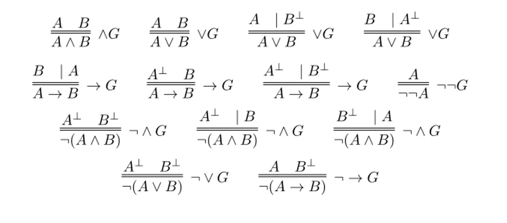
The propositional grounding rules are presented in Table 2. They corre-spond to the grounding rules in [26], but their presentation is different. Firstly, we do not use a unique rule for negation, as in [26], but we use separate rules for negated conjunctions, disjunctions, implications, and for double negations. This enables us to avoid side conditions on the propositional rules. Secondly, we use the | separator instead of square brackets to distinguish between a pre-miss representing a ground and a prepre-miss representing a condition:14 in a rule application of the form
A | B C
A is the ground of C under the condition B. Notation aside, both the grounding rules of the calculus in [26] and the grounding rules in Table 2 are defined according to the following conditions (notation adapted):
D A B A ∧ B ∧I A ∧ B A ∧E A ∧ B B ∧E A A ∨ B ∨I B A ∨ B ∨I A ∨ B A..n .. C B..n .. C C ∨E n An .. .. B A → B → I n A → B A B → E An .. .. ⊥ ¬A ¬I n ¬A A ⊥ ¬E ⊥ A ⊥E ¬¬A A ¬¬E
where n ∈ N and D does not contain any arbitrary object name Table 1: Propositional Rules for Classical Logic
Definition 4.1 (Rules for Logical Grounding). A rule of the form A1 . . . An | B
C
is a grounding rule if, and only if, the following conditions are met: • Positive Derivability: the rule A1 . . . An
C is classically sound. • Negative Derivability: the rule ¬A1 . . . ¬An B
¬C is classically sound. • Immediateness: gc(A1, . . . , An, B) + 1 = gc(C) and the list A1, . . . , An, B
contains exactly one element G or G⊥ for each immediate g-subformula G of C.
4.2
Rules for the grounding operator
The propositional fragment of our logic does not only feature classical connec-tives, but also a grounding operator Gr. This operator enables us to construct formulae of the form Gr(Γ : A) stating that the formulae in Γ constitute the ground of the formula A. The introduction rule for the Gr operator is in Ta-ble 3. This rule enaTa-bles us to introduce Gr only if we have a legitimate grounding rule application to justify the resulting grounding formula. For instance, if we ground P ∧ Q by the atoms P and Q, we can infer the formula Gr(P, Q : P ∧ Q)
A B A ∧ B ∧G A B A ∨ B ∨G A | B⊥ A ∨ B ∨G B | A⊥ A ∨ B ∨G B | A A → B → G A⊥ B A → B → G A⊥ | B⊥ A → B → G A ¬¬A ¬¬G A⊥ B⊥ ¬(A ∧ B) ¬ ∧ G A⊥ | B ¬(A ∧ B) ¬ ∧ G B⊥ | A ¬(A ∧ B) ¬ ∧ G A⊥ B⊥ ¬(A ∨ B) ¬ ∨ G A B⊥ ¬(A → B) ¬ → G
Table 2: Propositional Grounding Rules
If .. .. Γ | .. .. C B
is a derivation, then the following is a derivation:
.. .. Γ | .. .. C B Gr(Γ | C : B) GrI
(the condition C might not occur)
Table 3: Introduction Rule for the Grounding Operator Gr stating that the atoms P and Q constitute the ground of P ∧ Q:
P Q
P ∧ Q ∧G Gr(P, Q : P ∧ Q) GrI
The elimination rules for the grounding operator Gr are presented in Table 4. The first two rules are justified by the fact that the grounding relation holds between truths. If, for instance, A grounds B, then both A and B must be true. This feature is usually referred to as the factivity of ground. If the ground has a condition, the condition must be obviously true as well. The last rule of Table 4 is needed to negate grounding statements that violate the immediateness condition of Definition 4.1. By using it we can, for instance, formally show that the formula P ∧ Q does not ground the atom P :
Gr(P ∧ Q : P )1
⊥ GrE⊥
¬Gr(P ∧ Q : P ) ¬I
Gr(Γ : A) A GrE Gr(Γ : A) G GrE Gr(∆ : A) ⊥ GrE⊥
where G ∈ Γ, and either gc(∆) + 1 6= gc(A) or ∆ does not contain exactly one element D or D⊥ for each immediate g-subformula D of A
Table 4: Elimination Rules for the Grounding Operator
since gc(P ∧ Q) = 1, gc(P ) = 0 and 1 + 1 6= 0. We can also formally show that, for instance, the atoms P and Q do not ground the conjunction R ∧ S:
Gr(P, Q : R ∧ S)1
⊥ GrE⊥
¬Gr(P, Q : R ∧ S) ¬I1
since the list “P, Q” does not consist of formulae among R, S, ¬R, ¬S.
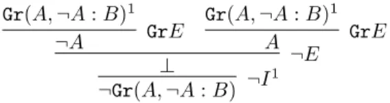
The negation of inconsistent grounding statements can be derived by factiv-ity. We know, for instance, that ¬Gr(A, ¬A : B) is true for any formulae A and B, since we can construct the following derivation:
Gr(A, ¬A : B)1
¬A GrE
Gr(A, ¬A : B)1
A GrE
⊥ ¬E
¬Gr(A, ¬A : B) ¬I1
And this can be similarly derived for any grounding statement in which grounds, condition, and consequence are inconsistent.
4.3
Ground-theoretic equivalences
We have now a propositional calculus that enables us to build grounding in-ferences and derive grounding formulae accordingly. Nevertheless, the calculus that we just introduced is too strict, and does not yet enable us to derive all the formulae we would like to. Indeed, as anticipated in Section 2, if we transform a formula D according to the laws of commutativity and associativity
B ∧ A ↔ A ∧ B (A ∧ B) ∧ C ↔ A ∧ (B ∧ C) B ∨ A ↔ A ∨ B (A ∨ B) ∨ C ↔ A ∨ (B ∨ C)
we obtain a formula D0 which is logically equivalent to D and, as argued in [6, 25], also equivalent to it as far as grounding is concerned. Therefore, we need some way to account for these ground-theoretic equivalences in the calculus, and derive the corresponding grounding statements. In order to do so,
we stipulate some equalities that enable us to freely transform formulae inside derivations according to the commutativity and associativity laws. To simplify our presentation, we introduce the following notation:
Definition 4.2 (Formula context). A formula context C[X] is a formula contain-ing a distcontain-inguished propositional atom X. For any formula A, by the notation C[A], we denote the formula obtained by replacing X with A in C[X].
Definition 4.3 (Derivations with Formula Equalities). We admit the following equivalences as equalities in the calculus:
C[B ∧ A] ≡ C[A ∧ B] C[(A ∧ B) ∧ C] ≡ C[A ∧ (B ∧ C)] C[B ∨ A] ≡ C[A ∨ B] C[(A ∨ B) ∨ C] ≡ C[A ∨ (B ∨ C)]
To be more precise, we can define the rules of the calculus as rules acting on equivalence classes with respect to ≡. For any list S0, S1, . . . , Sn of such
equivalence classes, a rule application
S1 . . . Sn
S0
is legal if there is a list of formulae A0, . . . , An such that Ai∈ Si and
A1 . . . An
A0
is an instance of a rule schemata.
For the sake of simplicity, inside derivations we will simply treat the equiv-alence relation ≡ as a syntactic equality, thus not distinguishing between ≡-equivalent formulae. Therefore, for instance, the following is a legal derivation:
A ∧ B1 (B ∧ A)1 (B ∧ A) → C C → E (B ∧ A) ∧ C ∧G Gr(A ∧ B, C : (B ∧ A) ∧ C) GrI B ∧ A → Gr(A ∧ B, C : (B ∧ A) ∧ C) → I 1
where we use the equivalence A ∧ B ≡ B ∧ A. As one can see, we can use a formula as if it were an equivalent one. In particular, the grounding rule uses its left premiss as the formula B ∧ A; the Gr introduction rule uses it as A ∧ B; and the → introduction rule uses it as B ∧ A again. Another example, using the fact that A ∨ (B ∨ C) ≡ (C ∨ B) ∨ A, is the following:
A ∨ (B ∨ C) D ((C ∨ B) ∨ A) ∧ D
Gr(A ∨ (B ∨ C), D : ((C ∨ B) ∨ A) ∧ D)
Notice that the ground-theoretic equivalences enforce the uniqueness of the ground. Indeed, if G and G0 occur as the premiss of a grounding rule with conclusion C, and G ≡ G0, C does not have two distinct grounds, as the calcu-lus treats G as completely undistinguishable from G0.
A[x/y] ∀yA ∀I
∀yA A[t/y] ∀E
x does not occur free in any hypothesis on which A[x/y] depends
A[t/y]
∃yA ∃I ∃yA
A[x/y]n .. .. B B ∃E n
x does not occur in B and in any hypothesis H 6= A[x/y] on which B depends
A[x/y] A[a/y] aI
A[t/y] A[εyA/y] εI
x does not occur free in any hypothesis on which A[x/y] depends where n ∈ N, x and y are variables, t is any term,
and a is a name for an arbitrary object Table 5: Predicative Rules for Classical Logic
4.4
Logical and grounding predicative rules
We can now extend the propositional calculus with the logical and grounding rules for quantifiers, arbitrary object names, and the ε-symbol.
The predicative logical rules are presented in Table 5 and include natural deduction rules for first-order quantifiers [35, Chapter 2, Section 1], a rule for arbitrary objects, and a rule for εxA. Let us focus on the less common rules. The rule
A[x/y] A[a/y]
enables us to introduce a name for an arbitrary object and, in particular, to infer that a property A(x) holds for an arbitrary object a if A(x) can be derived without using any hypothesis on the variable x. If we have no assumptions on x, indeed, the derivation of A(x) shows us that A(x) holds for any object. We make this explicit by introducing the name a for an arbitrary object.
The term εxA, briefly introduced in Section 2, denotes an indeterminate object for which A(x) holds, if there is one. Technically, we can see ε as an operator that, when given the formula A(x) as argument, chooses an element that satisfies A(x), if there is one. For obvious technical reasons, if there is no object for which A(x) holds, then εxA denotes an object for which A(x) does
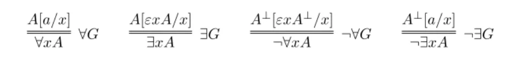
A[a/x] ∀xA ∀G A[εxA/x] ∃xA ∃G A⊥[εxA⊥/x] ¬∀xA ¬∀G A⊥[a/x] ¬∃xA ¬∃G
where x is a variable and a is an arbitrary object name Table 6: Grounding Rules for Quantifiers
not hold. Hence, the behaviour of εxA is formalized by the axiom ∃xA ↔ A[εxA/x]
and, from a proof-theoretical perspective, by the following two rules: A[εxA/x]
∃xA
A[t/x] A[εxA/x]
Indeed, if A(x) holds for the object picked by ε, it is obvious that there exists one object for which A(x) holds: the one picked by ε ! And hence we can infer ∃xA. If, on the other hand, there is a term t for which A(x) holds, we know that ε will be able to pick an object for which A(x) holds, and the rule above on the right guarantees us that ε will do so. Since the rule above on the left is just an instance of the introduction rule for ∃, we do not need to add it to the calculus.
In Table 6 we present the grounding rules for quantifiers. The rules for the existential and universal quantifier have been explained in Section 2.15 As for
the rules for negated quantifiers, their justification is as follows. The reasoning captured by the rule ¬∀G is very similar to the one captured by ∃G. Indeed, A⊥[εxA⊥/x] implies ∃xA⊥ because it guarantees that there is an object for which A⊥(x) holds. But this in turn implies that A(x) does not hold for all objects, and hence that ¬∀xA is true. The rule ¬∃G, on the other hand, relies on the same principles on which the rule ∀G is based. If A⊥[a/x] is true and a is a name for an arbitrary object, then A⊥(x) holds for all objects. Therefore, there is no object for which A(x) holds and ¬∃xA is true.
Now that we introduced and discussed all the required rules, we can formally define the notion of derivation (which is a standard one), and the notion of formal explanation.
Definition 4.4 (Derivations and Formal Explanations). Derivations are induc-tively defined as follows:
• Any formula A is a derivation of A with hypothesis A.
15Note that we cannot define a grounding rule for the universal quantifier by using the
ε-symbol, since such a rule would inevitably rely on reductio ad absurdum, but this principle is not admissible in a grounding derivation since it would make the argument formalized by the derivation an indirect one: one which does not prove the conclusion by a direct analysis of its components.
• If
Γ .. .. A is a derivation of A with hypotheses Γ, then
–
Γ..0 .. A B r
is a derivation of B with hypotheses Γ0 if r is an application of one of the rules in Table 1, 3, 4 or 5, and Γ0 contains all hypotheses in Γ which are not discharged by r.
– Γ .. .. A B rG
is a derivation of B with hypotheses Γ if rG is an application of one of the rules in Table 2 or 6.
• If Γ .. .. A ∆ .. .. B
are derivations of A and B with hypotheses Γ and ∆ respectively, then – Γ.. .. A ∆..0 .. B C r
is a derivation of C with hypotheses Γ ∪ ∆0 if r is an application of one of the rules in Table 1 or 5, and ∆0 contains all hypotheses in ∆ which are not discharged by r.
– Γ .. .. A ∆ .. .. B C rG
is a derivation of C with hypotheses Γ ∪ ∆ if rG is an application of one of the rules in Table 2.
A formal explanation is a derivation that only contains grounding rule ap-plications.
Before exemplifying how the grounding rules for quantifiers and negated quantifiers are employed, we formally show that they comply with our conditions on grounding rules. We do this by proving that these rules meet the criteria of positive and negative derivability and the complexity restrictions adopted for propositional grounding rules (Definition 4.1).
Theorem 4.1. All rules in Table 6 are rules for logical grounding (Defini-tion 4.1).
Proof. We start with positive derivability. We first prove that the rule (1) A[a/x]
∀xA ∀G
is classically sound. We do this by showing that whenever we have a derivation of A[a/x] from some hypotheses, we can derive ∀xA from the same hypotheses. Since a cannot occur in any open hypothesis, there must be a derivation δ of A[a/x] in which the name a has been introduced by some rule applications
B1[y1/x]
B1[a/x]
aI . . . Bn[yn/x] Bn[a/x]
aI
where each yi does not occur in any hypothesis on which Bi[yi/x] depends. We
construct a derivation δ0 by applying the following three operations to δ: first, we rename the bound variables in such a way that no ε-symbol binds a variable among y1, . . . , yn; second, we replace all occurrences of a in δ by a fresh variable
y; third, we replace all free occurrences of y1, . . . , yn in δ by the same variable
y. After the substitutions, the rule applications introducing a become trivial inferences of the form
Bi[y/x]
Bi[y/x]
We construct a derivation δ00 by eliminating them from δ0. Now, since a cannot occur in open hypotheses and since the rule applications imposing eigenvariable conditions on y1, . . . , yn do not occur in δ00 anymore, the fresh variable y does
not violate any eigenvariable condition in δ00. Since, moreover, we replaced a, y1, . . . , yn everywhere, all rule applications of one of the following forms
A[t/z] A[εzA/z] εI A[εzA/z] ∃zA ∃G A⊥[εz¬A⊥/z] ¬∀zA ¬∀G
became inferences of the following forms, respectively: (A[t/z])τ (A[εzA/z])τ (A[εzA0/z])τ (∃zA)τ (A⊥[εzA⊥/z])τ (¬∀zA)τ
where τ is the substitution [y/a][y/y1] . . . [y/yn]. Since, by renaming, z /∈
{y, y1, . . . , yn}, we can permute the substitution τ and obtain the following
rule applications, respectively: (Aτ )[(tτ )/z]
(Aτ )[εz(Aτ )/z] εI
(Aτ )[εz(Aτ )/z]
∃z(Aτ ) ∃G
(A⊥τ )[εz(A⊥τ )/z]
Therefore, δ00is a legal derivation of A[y/x]. Moreover, since a and y1, . . . , yndo
not occur in any open hypothesis of δ, y does not occur in any open hypothesis of δ00. Therefore, δ00 is a derivation of A[y/x] that does not depend on any hypothesis containing y, and we can derive ∀xA by
A[y/x] ∀xA The rule
(2) A[εxA/x] ∃xA
is clearly sound since since A[εxA/x] → ∃xA is one direction of the axiom that characterizes the ε-symbol.
Consider now the rule
(3) A
⊥[εxA⊥/x]
¬∀xA
By Definition 3.6, from any derivation of A⊥[εxA⊥/x] we can obtain a derivation of ¬A[εx¬A/x]. Since the implication ¬A[εx¬A/x] → ∃x¬A is one direction of the axiom characterising ε and the implication ∃x¬A → ¬∀xA is valid, we have that the rule is sound.
Consider now the rule
(4) A
⊥[a/x]
¬∃xA
By Definition 3.6, from any derivation of A⊥[a/x] we can obtain a derivation of ¬A[a/x] with no new hypotheses. Hence, as shown for rule (1), we can derive ∀x¬A. But since ∀x¬A → ¬∃xA, we have that the rule is classically sound.
Let us now move to negative derivability. As for rule (1), we showed above that we can derive ∀x¬A if we have a derivation of ¬A[a/x]. Negative derivabil-ity follows because the implication ∀y¬A → ¬∀yA is valid. As for rule (2), since ∃xA → A[εxA/x] is valid—it is one direction of the axiom characterising ε—we can obtain by contraposition that ¬A[εxA/x] → ¬∃xA is valid. Hence, we can derive ¬∃xA from ¬A[εxA/x] and thus show that negative derivability holds. As for rule (3). From ¬(A⊥[εxA⊥/x]) we can derive A[εx¬A/x]. Moreover, from ∃x¬A → ¬A[εx¬A/x]—which is one direction of the axiom characterising ε—we can obtain by contraposition ¬¬A[εx¬A/x] → ¬∃x¬A. Therefore, we can de-rive ¬∃x¬A from A[εx¬A/x] using the validity of A[εx¬A/x] → ¬¬A[εx¬A/x]. Negative derivability holds because ¬∃x¬A implies ¬¬∀xA. We conclude with rule (4), first notice that by Definition 3.6 we can derive A[a/x] from ¬(A⊥[a/x]). We can then see that negative derivability holds because from A[a/x] we can derive ∃xA and from this, ¬¬∃xA.
Finally, we check immediateness. First notice that, by Definition 3.5, it holds for any formula A that gc(A) = gc(A[t/x]) for any term t. Moreover, by Defintions 3.6 and 3.5, we have that for any formula A, gc(A) = gc(A⊥). Hence, by Definition 3.5, we have that gc(∀yA) = gc(∃xA) = gc(¬∀xA) = gc(¬∃yA) =
gc(A) + 1. By concatenating all these equalities, we can see that immediateness holds for the rules (1), (2), (3) and (4).
Notice that, since the equivalence A[εx¬A/x] ↔ ∀xA holds, we can use the the ε-symbol also to define the behaviour of the universal quantifier. Since, moreover, A[εx¬A/x] is logically simpler than ∀xA, the former formula could also constitute a reasonable candidate for the ground of the latter. Nevertheless, the implication from A[εx¬A/x] to ∀xA essentially relies on an argument by double negation elimination,16 and the arguments of this kind are tantamount
to arguments by reduction to absurdity—also called apagogic proofs—which are generally not considered suitable means for grounding truths. Proofs by reduction to absurdity, indeed, do not show in a direct way that their conclusion is true, but they do it in a roundabout way which does not match the idea that a ground should constitute a direct simplification or clarification of its consequence. Bolzano, for instance, states in [4, §530] that “the propositions by which an apagogic proof supports the propositions it is supposed to prove can never represent its objective ground.” Therefore, we do not employ the ε-symbol to define the grounds of universal and negated existential formulae but we employ names for arbitrary objects instead.
4.5
Examples
We now present some examples of derivations containing the new grounding rules for quantifiers. The first one is the following:
n = n axiom n + 1 6= 0 axiom
n = n ∧ n + 1 6= 0 ∧G | n = n axiom n 6= n ∨ (n = n ∧ n + 1 6= 0) ∨G
Note that n + 1 6= 0 and n = n are instances of arithmetical axioms. Hence, the derivation does not depend on any hypothesis but starts with the assertion of these two truths. We indicate this by the three inferences labeled “axiom” which have no premisses.
In this derivation, we start from the truths n = n and n + 1 6= 0 to ground their conjunction n = n ∧ n + 1 6= 0. Then we have that n = n ∧ n + 1 6= 0 is the ground of the disjunction n 6= n ∨ (n = n ∧ n + 1 6= 0) under the condition that the first disjunct n 6= n does not hold, or, equivalently, that n = n holds. Technically, n = n is the condition of the ∨G rule application since n 6= n is defined as ¬n = n and thus (n 6= n)⊥ is exactly n = n.
Since the derivation above depends on no hypothesis but only on axiom instances, we can introduce an arbitrary object name a instead of the variable n and obtain a 6= a ∨ (a = a ∧ a + 1 6= 0). Thus, we can ground the universal 16The formula A[εx¬A/x] is true if and only if ¬∃x¬A is true, and ¬∃x¬A is equivalent to
closure ∀n(n 6= n ∨ (n = n ∧ n + 1 6= 0)) of n 6= n ∨ (n = n ∧ n + 1 6= 0): n = n axiom n + 1 6= 0 axiom n = n ∧ n + 1 6= 0 ∧G | n = n axiom n 6= n ∨ (n = n ∧ n + 1 6= 0) ∨G a 6= a ∨ (a = a ∧ a + 1 6= 0) aI ∀n(n 6= n ∨ (n = n ∧ n + 1 6= 0)) ∀G
In the following example, we ground the universal formula ∀x(x = x → x = x) and we derive the statement expressing that its ground is a = a → a = a:
x = x axiom | x = x axiom x = x → x = x → G
a = a → a = a aI ∀x(x = x → x = x) ∀G
Gr( a = a → a = a : ∀x(x = x → x = x) ) GrI
The → G rule application corresponds to the fact that the true consequent x = x of the implication x = x → x = x is the ground of this implication under the condition that the antecedent, x = x again, is true.17 Since we have grounded
x = x → x = x without using any hypothesis on x, we can derive that a = a → a = a holds for an arbitrary object a. This implies that x = x → x = x holds universally, and hence grounds ∀x(x = x → x = x). After having grounded the universal statement on the individual statement about the arbitrary object a, we can derive the formula Gr( a = a → a = a : ∀x(x = x → x = x) ) which expresses that the grounding relation holds between the two statements.
Let us consider now an example for the existential grounding rule. Suppose that we want to ground the formula ∃x(x = b ∨ x = c), where b and c are constants such that b 6= c. Here is the resulting grounding derivation:
b = b axiom | . . . ¬(b = c) b = b ∨ b = c ∨G εx(x = b ∨ x = c) = b ∨ εx(x = b ∨ x = c) = c εI ∃x(x = b ∨ x = c) ∃G Gr( εx(x = b ∨ x = c) = b ∨ εx(x = b ∨ x = c) = c : ∃x(x = b ∨ x = c) ) GrI The derivation moves from the truth of b = b, which is just the instance of an axiom, to the truth of b = b ∨ b = c by a disjunction grounding rule. Since we can verify x = b ∨ x = c by substituting b for x, we know that there is some object which has the property expressed by x = b ∨ x = c, that is, the object denoted by b. Hence, we can introduce a term that stands for an indeterminate object that verifies x = b ∨ x = c. Such term is εx(x = b ∨ x = c). Notice that in 17The truth of the antecedent is a condition and not part of the ground because an
spite of the fact that the term εx(x = b ∨ x = c) is introduced here by proving the instance b = b ∨ b = c of the formula x = b ∨ x = c, it does specifically refer to b; indeed also c has the property expressed by x = b ∨ x = c and the term εx(x = b ∨ x = c), from a logical point of view, expresses no preference between b and c. This provides us with the generality required to completely determine the existential formula, and thus to ground it. The derivation then ends with the introduction of the Gr operator.
Let us consider now an example for the negated universal rule: 0 = 0 axiom ¬¬(0 = 0) ¬¬G ¬(0 6= 0) def. 6= εn(¬(n 6= 0)) 6= 0 εI ¬∀n(n 6= 0) ¬∀G Gr( εn(¬(n 6= 0)) 6= 0 : ¬∀n(n 6= 0) ) GrI
In this derivation, we first ground ¬¬(0 = 0) by the axiom instance 0 = 0. This shows, in turn, that ¬(0 6= 0) is true, by definition of 6=. Now we have one n that verifies ¬(n 6= 0) and we can introduce the ε-term εn(¬(n 6= 0)) to denote an indeterminate number which is not different from 0. Since we showed that if we look for a number which is not different from 0, we find a number which actually has this property—that is, we showed that εn(¬(n 6= 0)) 6= 0 is true—we can finally use it to ground ¬∀n(n 6= 0) and to introduce the Gr operator accordingly.
We finally provide an example concerning the negated existential rule. Sup-pose that we want to ground the formula corresponding to the fact that there is no number which is equal to its successor. We can use the following argument. We consider an arbitrary number n. We assume that it is equal to its successor: n = n + 1. Then we reason as follows: if n = n + 1, then n + 0 = n + 1, and, by the left cancellation law, we can infer that 0 = 1, which is false. Hence n = n + 1 must be false. Therefore, there is no number which is equal to its successor because the number n we started with is an arbitrary number. The formal derivation has the following form:
n = n + 11 .. .. 0 = 1.. .. ⊥ ¬(n = n + 1) ¬I 1 ¬(a = a + 1) aI ¬∃x(x = x + 1) ¬∃G
Note that, from a technical point of view, n is arbitrary even though we assume that n = n + 1, because this assumption is discharged before we introduce a and ground the negated existential formula.
5
Semantics
A semantics for the theory of first-order, classical grounding is obtained by improving a semantics for classical logic with (i) an interpretation for the ε-terms and names for arbitrary objects, (ii) semantic clauses for the grounding connective. These two tasks are carried out in Section 5.1 and Section 5.2, respectively.
5.1
A semantics for the ε-term and the grounding
quan-tifier rules
In order to provide a semantics for the ε-calculus-fragment of the theory of first-order grounding, we follow [37], with a few modifications. Let us start with classical (Tarskian) semantics, defining a the notion of L-structure.
Definition 5.1 (L-structure). An L-structure M is a set that contains: • A non-empty set M 6= ∅ as its support.
• An object cM∈ M for every individual constant of L.
• An n-ary function fM: Mn 7−→ M for every n-ary function constant of
L.
• An n-ary relation RM⊆ Mn for every n-ary relation constant of L.
We now define a choice function relative to an M-structure, in order to interpret ε-terms (we will omit the subscript M when no confusion arises). Definition 5.2 (Choice function). For any L-structure M, an M-choice func-tion FM is a function FM : P(M ) 7−→ M s.t. for every ∅ 6= X ⊆ M ,
FM(X) ∈ X.
We then proceed to define varible assignments and their variants. Note that variable assignments associate elements of the domain to variables as well as to constants for arbitrary terms, thus treating the latter essentially as the former (this follows [10], but our framework for arbitrary objects is much simpler). Definition 5.3 (Variable assignments). For any L-structure M, an M-variable assignment (or simply assignment, for short) σM is a function from the
indi-vidual variables and the names for arbitrary objects of L to M .
Definition 5.4 (xi-variant variable assignments). For any L-structure M and
M-assignment σ, an M-assignment σ0 is an x-variant of σ if it is identical to
σ with the only possible exception of the value σ0 assigns to x.
We now define the denotation of L-terms and the satisfaction relation for L-formulae, relative to an L-structure M, an M-choice function F , and an M-assignment σ. In a standard Tarskian semantics, one would typically first
define denotation and then satisfiaction, where the former definition is incor-porated and employed in the latter. Due to the presence of ε-terms, however, it is more convenient to define denotation and satisfaction together, as a single simultaneous inductive definition (see [23], Lemma 1C.1, pp. 12-13).
Definition 5.5 (Denotation of L-terms, satisfaction for L-formulae). Let M be an L-structure, F be an M-choice function, and σ an M-assignment. For every L-term s and L-formula A:
• xM,F,σ= σ(x) • M, F, σ |= >, and M, F, σ 6|= ⊥ • cM,F,σ = cM • (f (t1, . . . , tn))M,F,σ= fM(tM,F,σ1 , . . . , tM,F,σn ) • M, F, σ |= s = t iff sM,F,σ= tM,F,σ • M, F, σ |= R(t1, . . . , tn) iff htM,F,σ1 , . . . , tM,F,σn i ∈ RM,F,σ
• (εxA(x))M,F,σ= F (A(x)M,F,σ), where
A(x)M,F,σ = {σ0(x) ∈ M | σ0 is an x-variant of σ and M, F, σ0|= A(x)}
• M, F, σ |= ∃xA(x) iff for a x-variant M-assignment σ0, M, F, σ0|= A(x)
• M, F, σ |= ∀xA(x) iff for all x-variant M-assignments σ0, M, F, σ0|= A(x)
Note that, unlike the original definition in [37], Definition 5.5 is purely Tarskian, in that it employs only variable assignments and x-variants, rather than adding new names to the language, for elements of the support.18
With a semantics for the language L at hand, we can proceed to define a notion of logical consequence.
Definition 5.6 (Logical consequence). A formula ϕ is a logical consequence of a set of formulae Γ, in symbols Γ |= ϕ, if:
• For every L-structure M and every M-choice function F and M-assignment σ, if M, F, σ |= Γ, then M, F, σ |= ϕ.
[37] shows that the above notion of consequence yields soundness and com-pleteness results for classical logic augmented with an extensional ε-calculus, that is a calculus featuring an extensionality axiom to the effect that the refer-ent of εxA only depends on the set of values of x which (under an assignmrefer-ent σ for a structure M) satisfy A(x). Zach’s proof covers our quantifier rules em-ploying ε-terms: our rules ∃g and ¬∀g (see Table 6) are instances of Zach’s rules Ax∃ and Ax∀ (see [37], p. 32). So, we can state the following result.
Theorem 5.1 (Soundness and Completeness). For every set of L-sentences Γ ∪ {A}:
Γ ` A, if and only if Γ |= A
Proof. See [37], Theorems 28 and 30.
5.2
A semantics for the grounding operator
Definition 5.7 (Satisfaction for grounding formulae). Let M be an L-structure, F be an M-choice function, and σ an M-assignment. |=∗gis the relation obtained
by closing the definition of |= under the following clause: M, F, σ |=gGr(Γ|C : B) iff (letting Γ = {A1, . . . , An})
(i) For every Ai ∈ Γ, M, F, σ |= Ai and M, F, σ |= C
(ii) M, F, σ |= B
(iii) A1, . . . , An |= B and
(iv) ¬A1, . . . , ¬An, C |= ¬B, and
(v) gc(A1, . . . , An, C) + 1 = gc(B) and the list A1, . . . , An, C contains
exactly one element G or G⊥ for each immediate g-subformula G of C.
Writing it down in extenso, the definition of |=∗gwould look exactly like
Def-inition 5.5, with every occurrence of |= replaced by |=∗g but, crucially, where |=
(and not |=∗
g) is employed in (i)-(iv). This is because the rules for the grounding
operator require the logical soundness of the inferences codified by (i)-(iv). Clauses (i) and (ii) are motivated by the factivity of ground—the idea that the grounding relation holds between truths. In this construal, factivity restricts the sentences that enter the grounding relation as interpreted by hM, F, σi to sentences classically satisfied in it. Any given triple hM, F, σi adjudicates whether a grounding claim follows from another grounding claim by looking at whether the grounds and its consequence are satisfied by hM, F, σi. Therefore, models can be used to reason about arbitrary grounding claims only in a way which exactly mirrors the calculus (this will be guaranteed by the Soundness and Completeness theorems that follow), as the examples in section 4.5 can be reproduced semantically (and this is not surprising, given the clauses (i)-(v) above).19
Clauses (iii)-(v) are easily seen to be the semantic counterpart of Definition 4.1, with semantic consequence employed rather than derivability. Given the completeness of the classical calculus, the two are extensionally equivalent.
The consequence relation |=∗
gis not the relation we need yet: as pointed out
in Sections 2 and 4.3, we need to include ground-theoretic equivalences which enable to treat syntactically distinct formulae as identical from the ground-theoretical point of view. This is done in the next definition.
Definition 5.8 (Satisfaction for grounding formulae, with equivalences). Let For/≡be the quotient of the L-formulae under ≡. |=gis the satisfaction relation
defined exactly as in Definition 5.7, but on P(For/≡) × For/≡.
We now extend the satisfaction relation for grounding formulae to a full consequence relation for the theory of grounding. As the calculus does not distinguish between ≡-equivalent formulae, we will formulate the next results for For rather than For/≡, but no confusion will arise from this.
Theorem 5.2 (Soundness). For every set of L-sentences Γ ∪ {A}: if Γ `gA, then Γ |=gA
Proof. It suffices to check that the rules governing the grounding operator are sound. We argue by induction on the length of the derivation. We start with the introduction rule for the grounding operator. Suppose we have introduced the grounding predicate as a result of an application of the rule GrI applied to a derivation of length n, concluding Gr(Γ | C : B) from
.. .. Γ | .. .. C B
where the latter is of length n. By hypothesis, the latter derivation ends with a grounding rule, i.e. Positive Derivability, Negative Derivability, and Immediate-ness (from Definition 4.1) hold. By the IH and Theorem 5.1, conditions (i)-(v) of Definition 5.7 hold as well, i.e. Γ, C |=gB.
Consider now the elimination rules. Suppose there is a derivation of length n + 1 ending with an application of GrE of GrE⊥ (conditions as in Table 4):
Σ .. . Gr(Γ : A) GrE A Σ .. . Gr(Γ : A) GrE G Σ .. . Gr(∆ : A) GrE⊥ ⊥
Consider GrE. By IH, Σ |=g Gr(Γ : A), and letting Σ = {S1, . . . , Sm}, Γ =
{G1, . . . , Gn}, for every L-structure M, M-choice F , and M-assignment σ:
(i) If M, F, σ |= S1, . . ., M, F, σ |= Sm, then M, F, σ |= A. This shows that
the first GrE rule is sound with respect to |=g.
(ii) If M, F, σ |= S1, . . ., M, F, σ |= Sm, then M, F, σ |= G1, . . ., M, F, σ |=
Gn. This shows that the second GrE rule is sound with respect to |=g.
Consider now GrE⊥. By IH, Σ |=g Gr(∆ : A). Let Σ = {S1, . . . , Sm}, ∆ =
{D1, . . . , Dn}, and assume that gc(D1, . . . , Dn) + 1 6= gc(A), or ∆ does not
contain exactly one element C or C⊥for each immediate g-subformula C of A.
(v) gc(D1, . . . , Dn) + 1 = gc(A) and ∆ contains exactly one element C or C⊥
for each immediate g-subformula C of A
Therefore, any L-structure M, M-choice function F , and M-assignment σ that satisfies Σ fails to satisfy Gr(∆ : A), i.e. Σ |=g⊥.
We can finally prove a Completeness Theorem. Since the proof adapts the usual Henkin-style argument, we will only highlight the less standard steps. Theorem 5.3 (Completeness). For every set of L-sentences Γ ∪ {A}:
if Γ |=gA, then Γ `gA
Proof. The strategy of the proof is the usual Henkin strategy, adapted to the relation |=g. More precisely:
1. Suppose that Γ |=gA
2. Then, Γ ∪ {¬A} is unsatisfiable.
3. Then, Γ ∪ {¬A} is inconsistent, i.e. Γ ∪ ¬A `g⊥.
4. Then, Γ `gA.
Steps 1-2 and 3-4 are almost immediate, and require only rules and semantic clauses for negation that are validated by the calculus and the semantics. The step from 2 to 3 requires a version of the Henkin construction.
• Henkin Lemma. For every consistent set Γ of L-formulae there is a con-sistent and saturated Γ0 ⊇ Γ. The proof proceeds as usual, by adding instances of ∃xA(x) → A(t) to Γ.
• Lindenbaum Lemma. For every consistent set Γ of L-formulae there is a consistent and complete Γ00 ⊇ Γ. The proof proceeds as usual, i.e. for every formula A, either A or ¬A is added to Γ.
• Derivability entails elementhood. Let Γ be a consistent, saturated, and complete set of L-formulae. For every L-formula A, if Γ `g A, then
A ∈ Γ.
• Canonical model construction. Following [37], let Γ be a consistent set of L-formulae. Let Γ∗be the saturated and complete extension of Γ obtained
by applying the Henkin and then the Lindenbaum Lemma to it. For any two L-terms s and t, let s ≈ t be the congruence defined by s = t ∈ Γ∗, i.e. Γ∗`gs = t. Put (where Ter is the set of L-terms):
[s]≈Γ∗ :={t ∈ Ter | s ≈Γ∗ t}}
Ter/≈Γ∗ is the quotient of Ter under ≈Γ∗. Let F be a choice function on
Ter/≈Γ∗ and, for every T ∈ Ter/≈Γ∗, define:
FΓ∗(T ) =
(
{s ∈ Ter | s ≈ εxA(x)}, if T = {[t]≈Γ∗ ∈ Ter/≈Γ∗| A(t) ∈ Γ ∗}
F (T ), otherwise
As [37] shows, FΓ∗ is a well-defined choice function on Ter/≈Γ∗. The
(quotient) canonical model of Γ∗is the structure MΓ∗ defined as follows:
- Its support is Ter/≈Γ∗.
- cMΓ∗ = [c]≈ Γ∗. - (f ([s1]≈Γ∗, . . . , [sn]≈Γ∗)) MΓ∗ = [f (s 1, . . . , sn)]≈Γ∗. - h[s1]≈Γ∗, . . . , [sn]≈Γ∗i ∈ R MΓ∗ iff R(s 1, . . . , sn) ∈ Γ∗.
Finally, let σΓ∗ be an MΓ∗-assignment.
• Canonical Model Lemma. Let Γ∗, M
Γ∗, FΓ∗, and σΓ∗ be as above. For
every L-formula A:
MΓ∗, FΓ∗, σΓ∗|=gA iff A ∈ Γ∗
Proof: By induction on the complexity of formulae. We only do the salient case, i.e. A = Gr(∆ : B) (where, for simplicity, ∆ does not contain any condition). Suppose MΓ∗, FΓ∗, σΓ∗ |=g Gr(∆ : B). Then, by Definition
5.7:
(i) For every Di∈ ∆, MΓ∗, FΓ∗, σΓ∗|= Di
(ii) MΓ∗, FΓ∗, σΓ∗ |= B
(iii) D1, . . . , Dn|= B and
(iv) ¬D1, . . . , ¬Dn |= ¬B, and
(v) gc(D1, . . . , Dn) + 1 = gc(B) and D1, . . . , Dn, B contain exactly one
element G or G⊥ for each immediate g-subformula G of B.
Conditions (i) and (ii) are well-defined, since MΓ∗is a classical structure,
even though the language includes the grounding operator. Formulae of the form Gr(∆ : B) are treated as propositional atoms by |=. By (i) and IH, for every Di ∈ ∆, Di∈ Γ∗. By (ii) and IH, B ∈ Γ∗as well. Moreover,
by (iii) and (iv), pure logic, and the completeness of the logical calculus: (iii)∗ Γ, D1, . . . , Dn` B
(iv)∗ Γ, ¬D1, . . . , ¬Dn ` ¬B
By (iii)∗, (iv)∗, and (v), we can conclude Γ∗ `g Gr(∆ : A) and by