Asymptotic analysis of small defects near a singular point in antiplane elasticity, with an application to the nucleation of a crack at a notch

HAL Id: hal-01152441

https://hal.archives-ouvertes.fr/hal-01152441

Submitted on 20 May 2015

HAL is a multi-disciplinary open access archive for the deposit and dissemination of sci-entific research documents, whether they are pub-lished or not. The documents may come from teaching and research institutions in France or abroad, or from public or private research centers.

L’archive ouverte pluridisciplinaire HAL, est destinée au dépôt et à la diffusion de documents scientifiques de niveau recherche, publiés ou non, émanant des établissements d’enseignement et de recherche français ou étrangers, des laboratoires publics ou privés.

point in antiplane elasticity, with an application to the

nucleation of a crack at a notch

Thi Bach, Tuyet Dang, Laurence Halpern, Jean-Jacques Marigo

To cite this version:

Thi Bach, Tuyet Dang, Laurence Halpern, Jean-Jacques Marigo. Asymptotic analysis of small defects near a singular point in antiplane elasticity, with an application to the nucleation of a crack at a notch. Mathematics and Mechanics of Complex Systems, International Research Center for Mathematics & Mechanics of Complex Systems (M&MoCS),University of L’Aquila in Italy, 2014, 2 (2), pp.141-179. �10.2140/memocs.2014.2.141�. �hal-01152441�

S’ESSA NON PASSA PER LE MATEMATICHE DIMOSTRAZIONI LEONARDO DA VINCI

Mathematics and Mechanics

of

Complex Systems

msp

vol. 2

no. 2

2014

THIBACHTUYET DANG, LAURENCEHALPERN ANDJEAN-JACQUESMARIGO

ASYMPTOTIC ANALYSIS OF SMALL DEFECTS NEAR A SINGULAR POINT IN ANTIPLANE ELASTICITY,

WITH AN APPLICATION TO THE NUCLEATION OF A CRACK AT A NOTCH

Vol. 2, No. 2, 2014

dx.doi.org/10.2140/memocs.2014.2.141 M\M

ASYMPTOTIC ANALYSIS OF SMALL DEFECTS NEAR A SINGULAR POINT IN ANTIPLANE ELASTICITY,

WITH AN APPLICATION TO THE NUCLEATION OF A CRACK AT A NOTCH

THIBACHTUYET DANG, LAURENCEHALPERN ANDJEAN-JACQUESMARIGO

We use matching asymptotic expansions to treat the antiplane elastic problem associated with a small defect located at the tip of a notch. In a first part, we develop the asymptotic method for any type of defect and present the sequential procedure which allows us to calculate the different terms of the inner and outer expansions at any order. This requires in particular separating in each term its singular part from its regular part. In a second part, the asymptotic method is applied to the case of a crack of variable length located at the tip of a given notch. We show that the first two nontrivial terms of the expansion of the energy release rate are sufficient to well approximate the dependence of the energy release rate on the crack length in the range of values of the length which are sufficient to treat the problem of nucleation. This problem is considered in the last part where we compare the nucleation and the propagation of a crack predicted by two different models: the classical Griffith law and the Francfort–Marigo law based on an energy minimization principle. Several numerical results illustrate the interest of the method.

1. Introduction

A major issue in fracture mechanics is how to model the initiation of a crack in a sound material; see [Bourdin et al. 2008]. There are two difficulties: the first one is to propose a law able to predict that nucleation; the second is a purely numerical issue. Indeed, it is difficult to compute with good accuracy the energy release rate associated with a crack of small length which appears at the tip of a notch; see [Marigo 2010]. The classical finite element method (FEM) leads to inaccurate

Communicated by Francesco dell’Isola.

This work was partially supported by the French Agence Nationale de la Recherche (ANR), under grant epsilon (BLAN08-2_312370) “Domain decomposition and multi-scale computations of singu-larities in mechanical structures”.

MSC2000: 35A15, 35B40, 35C20, 74A45, 74G70, 74R10.

Keywords: brittle fracture, variational methods, asymptotic methods, singularities.

results because of the overlap of two singularities which cannot be correctly cap-tured by this method: one is due to the tip of the notch; the other is due to the tip of the crack. A specific method of approximation based on asymptotic expansions is preferable as it is developed in analogous situations with localized defects; see for instance [Abdelmoula and Marigo 2000; Abdelmoula et al. 2010; Bilteryst and Marigo 2003; Bonnaillie-Noël et al. 2010; 2011; David et al. 2012; Geymonat et al. 2011; Leguillon 1989; Marigo and Pideri 2011; Vidrascu et al. 2012]. The first part of the present paper is devoted to the presentation of this matched asymptotic method (shortly, the MAM) in the case of a defect (which includes the case of a crack) located at the tip of a notch in the simplified context of antiplane linear elasticity. Therefore, our approach can be considered as a particular case of the previous works which have been devoted to the study of elliptic problems in corner domains, like [Dauge 1988; Dauge et al. 2010; Grisvard 1985; 1986]. However, a major difference is that we want to use these asymptotic methods to predict the nucleation or the propagation of defects (like cracks) near those singular points. The second and third parts of our paper will be devoted to this task. This requires, of course, to introduce a criterion of nucleation. This delicate issue has not received a definitive answer at the present time and it was considered for a long time as a prob-lem which could not be solved in the framework of Griffith’s theory of fracture [Bui 1978; Cherepanov 1979; Lawn 1993; Leblond 2003]. The main invoked reason is that the release of energy due to a small crack tends to zero when the length of the crack tends to zero; see [Chambolle et al. 2008; Marigo 2010]. Therefore, accord-ing to the Griffith criterion which states that the crack can propagate only when the energy release rate reaches a critical value characteristic of the material, no nucle-ation is possible because the energy release rate vanishes when there is no preexist-ing crack. This limitation of Griffith’s theory was one of the motivations which led Francfort and Marigo [1998] to replace the Griffith criterion by a principle of least energy, in the spirit of the original idea of [Griffith 1921]. It turns out that the princi-ple of least energy is really able to predict the nucleation of cracks in a sound body. However, as it was generically proved in [Chambolle et al. 2008; Francfort and Marigo 1998], the nucleation is necessarily brutal in the sense that a crack of finite length suddenly appears at a critical loading. Accordingly, we propose to revisit the problem of nucleation of a crack at the tip of a notch by comparing the two criteria. One of our goals is to use the MAM to obtain semianalytical expressions for the critical loading at which a crack appears and the length of the nucleated crack.

Specifically, the paper is organized as follows. Section 2 is devoted to the de-scription of the MAM on a generic antiplane linear elastic problem where the body contains a defect near the tip of a notch. We first decompose the solution into two expansions: the outer expansion is valid far enough from the tip of the notch while the inner expansion is valid in a neighborhood of the tip of the notch. These

expansions contain a sequence of inner and outer terms which are solutions of inner and outer problems and are connected by the matching conditions. Moreover each term contains a regular and a singular part. We explain how all the terms and the coefficients entering in their singular and regular parts are sequentially determined. The section finishes with an example where the exact solution is obtained in closed form and hence where we can verify the relevance of the MAM.

In Section 3, the MAM is applied to the case where the defect is a crack. Its main goal is to compute with good accuracy the energy release rate associated with a crack of small length near the tip of the notch. Indeed, it is a real issue in the case of a genuine notch (as opposed to a crack) because the energy release rate starts from 0 when the length of the nucleated crack is 0, then is rapidly increasing with the length of the crack before reaching a maximum and is finally decreasing. Accordingly, after the setting of the problem, the computation of the energy release rate by the FEM is described, and the reason why the numerical results are less accurate when the crack length is small is given. Then, the MAM is used to com-pute the energy release rate for small values of the crack length. As expected, the computation shows that, the smaller the size of the defect, the more accurate is the approximation by the MAM at a certain order. It even appears that very accurate results can be obtained by computing a small number of terms in the matched asymptotic expansions. We discuss also the influence of the angle of the notch on the accuracy of the results, this angle playing an important role in the process of nu-cleation (because, in particular, the length lmat which the maximum of the energy

release rate is reached depends on the angle of the notch). It turns out that when the notch is sufficiently sharp, i.e., sufficiently close to a crack, the first two nontrivial terms of the expansion of the energy release rate are sufficient to capture with very good accuracy the dependence of the energy release rate on the crack length.

In Section 4, we study the problem of crack nucleation at the tip of a notch. We first introduce the two competing evolution laws, i.e., the G-law and the FM-law: the first one is the usual Griffith’s law based on the criterion of critical energy release rate; the second is that introduced in [Francfort and Marigo 1998], which is based on the concept of energy minimization. We recall some general results previously established in [Marigo 2010] and extend them to the present case of a notch-shaped body in an antiplane setting. By virtue of the good approximation given by the MAM, we are able to solve the evolution problem in a quasiclosed form, the solution depending only on two coefficients that must be computed by the FEM. This permits a qualitative and quantitative comparison of the two laws.

+

N r

x

D

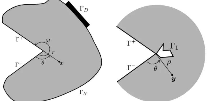
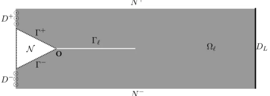
Figure 1. The domain l for the real problem.

+ N r x D + y 1

Figure 2. The domains 0 and 1 for, respectively, the outer

(left) and the inner (right) problems.

2. The real problem and its expansion by the matched asymptotic method 2.1. The real problem. Here, we consider a small geometrical defect of size l (like a crack or a void) located near the corner of a notch; see Figure 1. The geometry of the notch is characterized by its angle !; see Figure 2. The tip of the notch is taken as the origin of the space. We will introduce two scales of coordinates: the “macroscopic” coordinates x = (x1,x2) used in the outer domain, and the “microscopic” coordinates y = x/l = (y1,y2)used in the neighborhood of the tip of the notch where the defect is located; see Figure 2. In the case of a crack, the axis x1 is chosen in such a way that the crack corresponds to the line segment

The natural reference configuration of the sound two-dimensional body is 0,

while the associated body which contains a defect of size l is l. The part of the

boundary of l which is due to the defect is denoted by 0l; i.e.,

0l = @l\ @0, (1)

and 0l is contained in the disk of center (0, 0) and radius l. In the case of a crack, 0l

is the crack itself; i.e., 0l = (0, l) ⇥ {0}. The two edges of the notch are denoted by

0+ and 0 . To simplify the presentation, it is assumed that they are not modified by the introduction of the defect; see Figure 1. When using polar coordinates (r, ✓), the pole is the tip of the notch and the origin of the polar angle is the edge 0 . Accordingly, we have

r =|x|, 0 ={(r, ✓):0<r <r⇤, ✓= 0}, 0+= {(r, ✓) : 0 <r <r⇤, ✓= !}. (2) This body is made of an elastic isotropic material whose shear modulus is µ > 0. It is submitted to a loading such that the displacement field at equilibriumul be

antiplane; i.e.,

ul(x) = ul(x1,x2)e3,

where the subscript letter l is used as a reminder that the real displacement depends on the size of the defect. We assume that the body forces are zero and then ul must

be an harmonic function in order to satisfy the equilibrium equations in the bulk:

1ul= 0 in l. (3)

The edges of the notch are free while 0l is submitted to a density of (antiplane)

surface forces. Accordingly, the boundary conditions on 0l and 0±are

@ul @⌫ = 0 on 0 ±_, @ul @⌫(x) = g(y) l on 0l. (4)

In (4), ⌫ denotes the unit outer normal vector to l, and we assume that the

den-sity of (antiplane) surface forces depends on the microscopic variable y and has a magnitude of the order of 1/l.

The remaining part of the boundary of lis divided into two parts: 0Dwhere the

displacement is prescribed and 0N where (antiplane) surface forces are prescribed.

Specifically, we have

ul = f on 0D, @ul

@⌫ = h on 0N. (5)

The following proposition is a characterization of those functions which are har-monic in an angular sector and whose normal derivatives vanish on the edges of the sector. It is of constant use throughout the paper.

Proposition 1. Let r1 and r2be such that 0  r1 <r2  +1 and let$rr21 be the

angular sector

$r2

r1= {(r, ✓) : r 2 (r1,r2), ✓ 2 (0, !)}.

Then any function u which is harmonic in$r2

r1 and which satisfies the Neumann

condition @u/@✓ = 0 on the sides ✓ = 0 and ✓ = ! can be expanded as u(r, ✓) =a0ln(r) +d0+

X

n2N⇤

(anr n +dnrn )cos(n ✓), =⇡

!, (6)

where theanand thednconstitute two sequences of real numbers which are

char-acteristic of u.

Proof. Since the normal derivative vanishes at ✓ = 0 and ✓ = !, u(r, ✓) can be expanded in a Fourier series as

u(r, ✓) =X

n2N

fn(r) cos(n ✓).

In order that u be harmonic, the functions fn must satisfy r2fn00+r fn0 n2 2fn= 0

for each n. We easily deduce that f0(r) =a0ln(r)+d0and fn(r) =anr n +dnrn

for n 1. ⇤

2.2. The matching asymptotic method (MAM). We will write two asymptotic ex-pansions of ul in terms of the small parameter l. The inner expansion is valid in the

neighborhood of the tip of the notch, while the outer expansion is valid far from this tip. These two expansions will be matched in an intermediate zone.

2.2.1. The outer expansion. Far from the tip of the notch, i.e., for r l, ul does

not see the notch, and we assume that it can be expanded as ul(x) =X

i2N

li ui(x). (7)

In (7), even if this expansion is valid far enough from r = 0 only, ui _{must be}

defined in the whole outer domain 0which corresponds to the sound body; see

Figure 2 (left). Inserting this expansion into (3), (4), and (5) yields the sequence of problems for the ui_:

The first outer problem, i = 0: 8 > > > > > > > > < > > > > > > > > : 1u0_{= 0 in }0_, @u0 @⌫ = 0 on 0 +_{[ 0 ,} @u0 @⌫ = h(x) on 0N, u0_{= f (x) on 0} D. (8)

The other outer problems, i 1: 8 > > > > > > > > < > > > > > > > > : 1ui _{= 0 in }0_, @ui @⌫ = 0 on 0 +_{[ 0 ,} @ui @⌫ = 0 on 0N, ui _{= 0 on 0} D. (9)

Moreover, the behavior of ui _{in the neighborhood of r = 0 is singular and the}

singularity will be given by the matching conditions.

2.2.2. The inner expansion. Near the tip of the notch, i.e., for r ⌧ 1, we assume that the displacement field ul can be expanded as

ul(x) = ln(l)X i2N li wi(y) +X i2N li vi(y), y = x l. (10)

In (10), even if this expansion is valid only in the neighborhood of r = 0, the fields vi _{and w}i _{must be defined in the infinite inner domain 1. The domain 1}

is the infinite angular sector$1₀ of the (y1,y2)plane, from which the rescaled

defect of size 1 is removed; see Figure 2 (right). Accordingly, the rescaled bound-ary 01of the defect is

01= @1\ @$10 . (11)

(In the case of a crack, 01= (0, 1) ⇥ {0}.) Inserting this expansion into the set of

equations constituting the real problem yields the sequence of problems for the vi_:

The first inner problem, i = 0: 8 > > > > > < > > > > > : 1v0= 0 in 1, @v0 @✓ = 0 on ✓ = 0 and ✓ = !, @v0 @⌫ = g( y) on 01. (12)

The other inner problems, i 1: 8 > > > > > < > > > > > : 1vi = 0 in 1, @vi @✓ = 0 on ✓ = 0 and ✓ = !, @vi @⌫ = 0 on 01. (13)

The wi _{must satisfy, for every i 0, the same equations as the v}i _{for i 1. To}

complement the set of equations, the behavior at infinity of the vi _{and the w}i _must

be included. It is obtained by the matching conditions from the outer problems. 2.2.3. Matching conditions. In any sector$r2

0 with l ⌧ r2⌧ 1, the displacement

fields ui _{in the outer expansion are harmonic and satisfy homogeneous Neumann}

boundary conditions on the edges. Therefore Proposition 1 applies, and ui(x) =ai₀ln(r) +di₀+X

n2N⇤

(ai_nr n +di_nrn )cos(n ✓). (14) As for the inner expansion, the displacement fields vi _{and w}i _{are harmonic in the}

sector$1₁ of the y plane and satisfy homogeneous Neumann boundary conditions

on the edges. Therefore Proposition 1 applies, with the microscopic coordinates y and ⇢ = | y| = r/l replacing the macroscopic coordinates x and r:

vi(y) =ci₀ln(⇢) +bi₀+X n2N⇤ (ci_n⇢ n +bi_n⇢n )cos(n ✓), (15) wi(y) =ei₀ln(⇢) +f₀i+X n2N⇤ (ei_n⇢ n +f_ni⇢n )cos(n ✓). (16) The outer expansion and the inner expansion are both valid in any intermediate zone$r2

r1 such that l ⌧ r1<r2⌧ 1. Inserting (14) into the outer expansion (7)

with r = l⇢ leads to ul(x) = X i2N ln(l)li _ai 0 +X i2N li ✓ ai₀ln(⇢) +di₀+X n2N⇤ (ai+n_n ⇢ n +di n_n ⇢n )cos(n ✓) ◆ , (17) with the convention thatdi n_n = 0 when n > i. Inserting (15) and (16) into the inner

expansion (10) leads to ul(x) =X i2N ln(l)li ✓ ei₀ln(⇢) +f₀i +X n2N⇤ (ei_n⇢ n +f_ni⇢n )cos(n ✓) ◆ +X i2N li ✓_ci 0ln(⇢) +bi0+ X n2N⇤ (ci_n⇢ n +bi_n⇢n )cos(n ✓) ◆ . (18) Both expansions (17) and (18) are valid provided that 1 ⌧ ⇢ ⌧ 1/l. Identification of these expansions provides the connections between the coefficients of the inner and outer expansions described in Table 1.

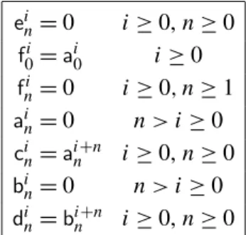
Remark 1. From Table 1 can be deduced that the fields wi _{are constant in the}

whole inner domain:

ei_n= 0 i 0, n 0 f₀i =ai₀ i 0 f_ni = 0 i 0, n 1 ai_n= 0 n > i 0 ci_n=ai+n_n i 0, n 0 bi_n= 0 n > i 0 di_n=bi+n_n i 0, n 0

Table 1. The relations between the coefficients of the inner and outer expansions given by the matching conditions.

Therefore, these fields will be determined once the constantsai₀ are known.

2.2.4. The singular behavior of the ui _{and the v}i_{. From the matching conditions}

can be read the behavior of ui _{in the neighborhood of r = 0 and the behavior of v}i

at infinity. In particular, the form of their singularities is visible, according to the following definition.

Definition 1. A field u defined in 0 is regular in 0 if u 2 H1(0); i.e., u 2

L2_(

0)and ru 2 L2(0)2. It is singular otherwise.

A field u defined in the unbounded domain 1 _{is regular in }1 _{if ru 2}

(L2_(1₎₎2_{and lim}

⇢_!1u(⇢, ✓) = 0. It is singular otherwise.

Remark 2. In other words, a field is regular if the associated elastic energy is finite. It is singular otherwise. In the case of the unbounded domain 1_{, a constant field}

has finite energy, but the condition at infinity is added in order to fix the constant and obtain the uniqueness in the forthcoming boundary value problems.

According to the analysis in the previous subsection, the field u0 _{can be}

ex-panded in a neighborhood of the tip of the notch as u0(x) =a0₀ln(r) +X

n2N

bn_nrn cos(n ✓). (20)

In the domain 0, ln(r) is singular, whereas rn cos(n ✓) is regular for n 0, in

the sense of Definition 1. Accordingly, u0 _{is split into its singular and regular parts}

as follows:

u0(x) = u0_S(x) + ¯u0(x), (21)

In the same way, for i 1, the field ui _{can be expanded in a neighborhood of the}

tip of the notch as ui_{(x) =a}i 0ln(r) + i X n=1 ai_nr n cos(n ✓) +X n2N bi+n_n rn cos(n ✓). (23)

Since r n _{cos(n ✓) is singular (for n 0) in the sense of Definition 1, u}i _{is split}

into its singular and regular parts as follows: ui_{(x) = u}i S(x) + ¯ui(x), (24) ui S(x) =ai0ln(r) + i X n=1 ai_nr n cos(n ✓), ¯ui 2 H1(0). (25)

For the fields vi _{of the inner expansion, the behavior at infinity comes into play.}

By virtue of the analysis in the previous subsection, the field vi _{for i 0 can be}

expanded for large ⇢ as vi(y) =ai₀ln(⇢) + i X n=0 bi_n⇢n cos(n ✓) +X n2N⇤ ai+n_n ⇢ n cos(n ✓). (26) The field ln(⇢) as well as the fields ⇢n _{cos(n ✓), for n 0, are singular in }1

in the sense of Definition 1 (even the constant field 1 corresponding to n = 0 is singular). Since the fields ⇢ n _{cos(n ✓) are regular when n 1, v}i _{is split into}

its singular and regular parts as follows:

vi(y) = vi_S(y) + ¯vi(y), (27) vi_S(y)=ai₀ln(⇢)+ i X n=0 bi_n⇢n cos(n ✓), r ¯vi2 L2(1), lim | y|!1¯v i_{(y)=0. (28)}

Remark 3. This analysis of the singularities shows that the singular parts of the fields ui _{and v}i _{will be known once the coefficientsa}i

nandbin are determined for

0  n  i.

2.2.5. The problems defining the regular parts ¯ui_{and ¯v}i_{. The singular parts (u}i S, viS)

are harmonic and satisfy the homogeneous Neumann boundary conditions on the edges of the notch. Therefore the regular parts are harmonic too, with data ex-pressed in terms of the singular fields.

The first outer problem, i = 0: Find ¯u0_{regular in } 0 such that 8 > > > > > > > > < > > > > > > > > : 1¯u0= 0 in 0, @¯u0 @⌫ = 0 on 0 +_{[ 0 ,} @¯u0 @⌫ = h @u0_S @⌫ on 0N, ¯u0_{= f u}0 S on 0D. (29)

The other outer problems, i 1: Find ¯ui _{regular in }

0such that 8 > > > > > > > > < > > > > > > > > : 1¯ui = 0 in 0, @¯ui @⌫ = 0 on 0 +_{[ 0 ,} @¯ui @⌫ = @ui_S @⌫ on 0N, ¯ui _{= u}i S on 0D. (30)

The first inner problem, i = 0: Find ¯v0_{regular in }1_{such that}

8 > > > > > < > > > > > : 1¯v0= 0 in 1, @¯v0 @⌫ = 0 on 0 +_{[ 0 ,} @¯v0 @⌫ = g @v_S0 @⌫ on 01. (31)

The other inner problems, i 1: Find ¯vi _{regular in 1 such that}

8 > > > > > < > > > > > : 1¯vi = 0 in 1, @¯vi @⌫ = 0 on 0 +_{[ 0 ,} @¯vi @⌫ = @vi_S @⌫ on 01. (32)

Consider first the outer problems. The well-posedness is a direct consequence of classical results for the Laplace equation:

Proposition 2. Let i 0. For a given singular part ui

S, i.e., if the coefficientsainare

known for all n such that 0  n  i, then there exists a unique solution ¯ui _{of (30)}

(or of (29) when i = 0). Consequently, the coefficientsbi+n_n are then determined

As for the inner problems, since they are Neumann problems (except for the condition at infinity), defined in an infinite domain, more care must be taken. The well-posedness is ensured by a compatibility condition, as stated in Proposition 3. Proposition 3. Let i 0. For given bi_n with 0  n  i, there exists a regular

solution ¯vi _{for the i-th inner problem if and only if the coefficienta}i

0is such that a0₀= 1 ! Z 01 g(s) ds, ai₀= 0 for i 1. (33)

Moreover, if this condition is satisfied, then the solution is unique and therefore the coefficientsai+n_n are determined for all n 0.

Proof. The inner problems are pure Neumann problems in which no Dirichlet boundary conditions are imposed on the vi _{except for the condition at infinity.}

Consequently, they admit a solution (if and) only if the Neumann data satisfy a global compatibility condition. Let us reestablish that condition. Let R _{be the}

part of 1 _{included in the ball of radius R > 1; i.e., }R _{= 1\ { y : | y| < R}.}

Consider first the case i = 0. Integrating the equation 1v0_{= 0 over }R _{and using}

the boundary conditions leads to 0 = Z @R @v0 @⌫ ds = Z ! 0 @v0 @⇢ (R, ✓)R d✓ + Z 01 g(s) ds. (34) Using (26) yields R@v0 @⇢ (R, ✓) =a 0 0+ X n2N⇤ n c0_nR n +b0_nRn cos(n ✓). SinceR!

0 cos(n ✓) d✓ = 0 for all n 1, after inserting in (34), the desired condition

for a0₀ appears. For i 1, the same process is applied, and the integral over 01

vanishes, yielding the desired condition.

If the compatibility condition (33) is satisfied, then the existence of a regular solution for ¯vi _{is obtained by standard arguments. Note however that, since r ¯v}i

belongs to L2_(1_{), ¯v}i _{tends to a constant at infinity and this constant is fixed to 0}

by the additional regularity condition. As far as the uniqueness is concerned, the solution of this pure Neumann problem is unique up to a constant and the constant is fixed by the condition that ¯vi _{vanishes at infinity.}

Once vi_{is determined, the coefficientsa}i+n

n are obtained by virtue of Proposition 1

and (26). ⇤

Remark 4. If the forces applied to the boundary of the defect are equilibrated, i.e., ifR₀₁g(s) ds = 0, then all the coefficientsai₀ vanish and hence the terms in ln(l)

disappear in the inner expansion. There are no more logarithmic singularities in the ui _{and the v}i_.

2.2.6. The construction of the outer and inner expansions. Recall the relationship between the coefficients (anj,bnj)and the singular and regular parts of the uj and vj:

uj = uSj + ¯uj, uSj ! anj _n=0j , ¯uj ! bnj+n n 0,

vj = v_Sj+ ¯vj, v_Sj ! a₀j, b_nj _n=0j , ¯vj ! a_nj+n _{n 0}.

(35) All the coefficientsa₀j vanish, except fora0₀, which is given by (33).

The scheme of the algorithm is the following. Suppose i 1, and uj _{and v}j _are

known for 1  j  i 1. The order of operations at step i is the following: (1) ui_Sis determined by ( ¯vi n₎

1ni,

(2) ¯ui _{is determined by u}i S,

(3) vi

Sis determined by ( ¯ui n)0ni,

(4) ¯vi _{is determined by v}i S.

Details are given below. Initialization:

(S1) Definea0₀by (33), and hence u0_S by (22).

(S2) From u0

S, define ¯u0 by (29), and hence u0= u0S+ ¯u0is determined.

(S3) Definebn_n for n 0 from (20) as the coefficients of ¯u0; see the next subsection

for the practical method. Hence, v0

S=a00+b00ln(⇢) is determined from (28).

(S4) From v0

S, ¯v0is computed by (31), and hence v0= v0S+ ¯v0is determined.

(S5) Definean_nfor n 1 from (26) as the coefficients of ¯v0; see the next subsection

for the practical method.

For i 1, suppose that uj _{and v}j _{have been determined, together with the}

coefficients in (35), for 0  j  i 1.

(R1) Sinceai_{0= 0, and writing, for 1  n  i,}ai_n=a(ni n)+n, uiS is given by (25),

where the coefficients are determined by those of the ¯vj _{for 1  j  i 1.}

(R2) ¯ui _{is obtained by solving (30).}

(R3) The coefficientsbi+n_n for n 0 are extracted from ¯ui in (23) and (24); see the

next subsection for the practical method.

(R4) Sinceai₀= 0, and usingbi_n=bnj+nwith j = i n, vi_Sis determined from (28).

(R5) ¯vi _{is obtained by solving (32).}

(R6) ui _{and v}i _{are obtained by summing the singular and regular parts.}

ai_n/bi_n i = 0 i = 1 i = 2 i = 3 i = 4

n = 0 (33)/Outer 0 0/Outer 1 0/Outer 2 0/Outer 3 0/Outer 4

n = 1 0 Inner 0/Outer 0 Inner 1/Outer 1 Inner 2/Outer 2 Inner 3/Outer 3

n = 2 0 0 Inner 0/Outer 0 Inner 1/ Outer 1 Inner 2/Outer 2

n = 3 0 0 0 Inner 0/Outer 0 Inner 1/Outer 1

n = 4 0 0 0 0 Inner 0/Outer 0

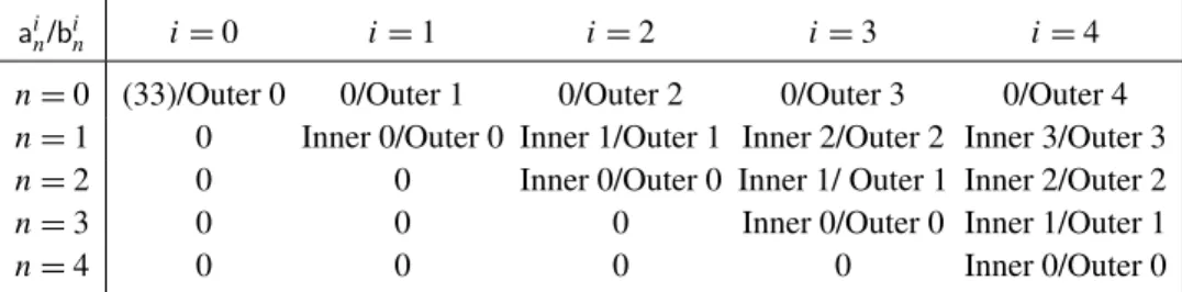
Table 2. Summary of the inductive method to obtain the coeffi-cientsai_nandbi_n: in the corresponding cell is indicated the problem

which must be solved.

2.2.7. The practical method for determining the coefficientsai_nandbi_n for 0  n  i.

Throughout this section,#r denotes the arc of the circle of radius r starting on 0

and ending on 0+_:

#r= {(r, ✓) : 0  ✓  !}.

The coefficientsai_n andbi_n can be obtained by path integrals (which are path

inde-pendent) as asserted in the following proposition.

Proposition 4. Let i 0. Assume that ¯vi _{and ¯u}i _{are known. Then:}

(1) For n 1, ai+n_n is given by the following path integral over #⇢, which is

independent of ⇢ provided that ⇢ > 1:

ai+n_n =2⇢ n ! Z ! 0 ¯v i_{(⇢, ✓ )cos(n ✓) d✓. (36)}

(2) For n 0, bi+n_n is given by the following path integral over #r, which is

independent of r provided that 0 < r < r⇤_:

bi₀= 1 ! Z ! 0 ¯u i_(r,✓)d✓, bi+n_n =2r n ! Z ! 0 ¯u i_{(r,✓)cos(n ✓)d✓ for n 1. (37)}

Proof. The proofs are identical for the two families of coefficients and only that concerningbi+n_n will be given. By (23), ¯ui is given for 0 < r < r⇤by

¯ui(r, ✓) =X

p2N

bi+p_p rp cos(p ✓),

which is for fixed r the Fourier series of ¯ui_{(r, · ). Formulas (37) follow. ⇤}

2.3. Verification in the case of a small cavity. This subsection is devoted to the verification of the construction of the matched asymptotic expansion (MAE) pre-sented in the previous subsections on an example where the exact solution is obtained in a closed form and hence can be directly expanded. Specifically, we consider a Laplace problem posed in a domain which consists of an angular sector

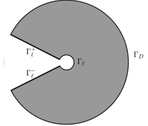
D +

Figure 3. The domain l in the case of a cavity.

delimited by two arc of circles. The radius of the outer circle is equal to 1 while the radius of the inner circle is l; see Figure 3. Thus,

l = {x = r cos ✓e1+ r sin ✓e2: r 2 (l, 1), ✓ 2 (0, !)}.

The sides of the notch and the inner circle are free and hence the boundary conditions on those parts of the boundary are

@ul

@⌫ = 0 on 0

+

l [ 0l [ 0l, (38)

where 0_l±= {(r, ✓) : l < r < 1, ✓ = 0 or !}, 0l= {(r, ✓) : r = l, 0  ✓  !}. (Note

that 0_l± depend on l, contrary to the assumption made in the remaining part of the paper. But that has no influence on the results.) The displacement is prescribed on the outer boundary 0D so that

ul(x) = cos ✓ on 0D, =⇡

!. (39)

Note that 0N is empty. Assuming that there is no body force, the exact solution of

this antiplane elastic problem is given by ul(x) =✓ l 2 1 + l2 r + 1 1 + l2 r ◆ cos ✓. (40)

Inserting the Taylor series of 1/(1+l2 ₎₌P

i2N( 1)i(l2 )i for l < 1, the expansion

of ul at a givenx takes the form

ul(x) = r cos ✓ +

X

n2N⇤

Thus (41) corresponds to the outer expansion where the odd terms vanish and the even terms are given by

u0_{(x) = r cos ✓, u}2n_{(x) = ( 1)}n_{(r r ) cos ✓ for all n 1. (42)}

To obtain the inner expansion, replace r by l⇢ in (40), to get ul(ly) = l

1 + l2 (⇢ + ⇢ ) cos ✓. (43)

Inserting the Taylor series as before, the expansion of ul(ly) is given by

ul(ly) =X n2N

( 1)nl(2n+1) (⇢ + ⇢ ) cos ✓, (44) which corresponds to the inner expansion where the even terms vanish and the odd terms are given by

v2n+1(y) = ( 1)n(⇢ + ⇢ ) cos ✓ for all n 0. (45) It remains to be checked that the procedure described in the previous subsec-tions yields the same coefficients. Since g = 0, ai₀ = 0 for all i 0 and there

is no logarithmic singularity; see Remark 4. The details for the first steps of the procedure are given below.

(S1) By (33),a0₀= 0 and hence u0_S= 0.

(S2) Hence (29) becomes: 1u0_{= 0 in }

0, @u0/@✓= 0 on ✓ 2 {0, !}, u0= cos ✓

on r = 1. The unique solution in H1_(

0)is u0given by (42).

(S3) By (37),b1₁= 1 andbn_n= 0 for n 6= 1. Hence v0_S= 0.

(S4) Since v0

S= 0 and g = 0, (31) gives ¯v0= 0 and hence v0= 0.

(S5) By (36),an_{n= 0 for n 1.}

(S6) By (25), u1 S= 0.

(S7) By (30), ¯u1_{= 0 and hence u}1_{= 0.}

(S8) By (37),bn+1_{n = 0 for all n. Hence v}1_{S= ⇢ cos ✓.}

(S9) Hence (32) for i = 1 becomes: 1¯v1_{= 0 in }1_{, @ ¯v}1_{/@✓= 0 on ✓ 2 {0, !},}

@¯v1/@⇢= cos ✓ on ⇢ = 1. The unique regular solution is ¯v1= ⇢ cos ✓ and hence v1 _{is given by (45).}

(S10) By (36),a2₁= 1 andan+1_n = 0 for n 6= 1.

(S11) By (25), u2

S= r cos ✓.

(S12) Hence (30) for i = 2 becomes: 1 ¯u2_{= 0 in }

0, @ ¯u2/@✓ = 0 on ✓ 2 {0, !}, ¯u2_{= cos ✓ on r = 1. The unique solution in H}1_(

0)is ¯u2= r cos ✓ and hence u2_{is given by (42).}

O D+ D N DL N+ N +

Figure 4. Definition of the cracked notch-shaped body l with

the various parts of the boundary.

Proceeding by induction, the expected expansions are finally recovered. The end of the verification is left to the reader.

3. Application to the case of a crack

3.1. Setting the problem. In this section, the method is applied to a defect which is a noncohesive crack. Specifically, let  be the rectangle ( H, L) ⇥ ( H, +H). Let ✏ be a given parameter in (0, 1),1_{= {x = (x}1,x2): H < x1 0, |x2|  ✏|x1|)}.

The notch-shaped body is 0= \1. Finally the cracked body l is obtained by

removing from 0the line segment 0l= (0, l) ⇥ {0}; see Figure 4.

The boundary 0Dwhere the displacement is prescribed corresponds to the sides

D±_{and DL, with boundary conditions}

ul(x) = 8 < : +H on D+_{= { H} ⇥ [✏ H, H],} H on D = { H} ⇥ [ H, ✏H], 0 on DL= {L} ⇥ [ H, H].

The remaining parts of the boundary (including the lips of the crack) are free; that is, @ul @x2 = ⇢0 on 0l= (0, l) ⇥ {0}, 0 on N±_{= ( H, L) ⇥ {±H}} and @ul @n =0 on 0 ±_{= {(x1,x2): H < x1<0, x2= ±✏x1}.}

Remark 5. The amplitude of the prescribed displacement is normalized to H so that ul has the dimension of a length. The fact that the amplitude is equal to the

height H has no importance in the present context of linearized elasticity. We will introduce a time-dependent amplitude of the prescribed displacement when we study the propagation of the crack. Then the prescribed displacement will take “reasonable” values, controlled by the toughness of the material.

Remark 6. The case ✏ = 0 corresponds to a body with an initial crack of length H and this limiting case is also considered in this paper. The case ✏ = 1 corresponds to a corner with an angle ⇡/2, the sides D±_{being reduced to the points ( H, ±H).}

This limiting case will not be considered here.

Remark 7. We only consider the case where the crack path is the line segment (0, L) ⇥ {0}. It is a rather natural assumption by virtue of the symmetry of the geometry and the loading. An interesting extension should be to consider non-symmetric geometry or loading and hence to take the direction of the crack as a parameter. This extension is reserved for future works.

We are in the case where g = 0 on 0l. Therefore, by virtue of Proposition 3, all

the coefficientsai₀vanish and there are no logarithmic singularities. Accordingly,

the solution can be expanded as follows:

Outer expansion: ul(x) = u0(x) + l u1(x) + l2 u2(x) + l3 u3(x) + · · · , Inner expansion: ul(x) = v0(y) + l v1(y) + l2 v2(y) + l3 v3(y) + · · · , with

=⇡

! and ! = 2⇡ 2 arctan(✏). (46)

By symmetry of the geometry and the loading, the real field ul is an odd function

of x2; i.e.,

ul(x1, x2)= ul(x1,x2), ul(r, ! ✓) = ul(r, ✓).

Therefore, all the fields ui_{, ¯u}i_{, v}i_{, ¯v}i _{admit the same symmetry. Therefore, by}

Proposition 4, all coefficientsbi+2n_2n andai+2n_2n vanish. Consequently, the odd terms

of the outer expansion and the even terms of the inner expansions vanish; i.e., u2i+1_{= 0 and v}2i _{= 0 for all i 2N. Finally, the solution admits the following}

expansions: Outer expansion: ul(x) =X i2N l2i u2i(x), (47) Inner expansion: ul(x) =X i2N

l(2i+1) _v2i+1_{(y). (48)}

By symmetry, the following coefficients vanish:

ai_n=0 when n or i n are even, bi_n=0 when n is even or i n is odd. (49)

Examine now the singularities of rul (in the sense that rul is not bounded)

(1) When ✏ > 0 and l = 0. Then ru0is infinite at the tip of the notch and in its

neighborhood has the form ru0(x) = b

1 1

r1 cos( ✓)er sin( ✓)e✓ + regular terms.

(2) When ✏ > 0 and l > 0. Then rul is no longer infinite at the tip of the notch

but becomes infinite at the tip of the crack, with the usual singularity in 1/pr; see [Bui 1978]. Specifically, rul has the form

rul(x) = Kl µp2⇡r0 ✓ sin ✓_✓0 2 ◆ er+ cos ✓_✓0 2 ◆ e✓ ◆ + regular terms. (50) In (50), (r0_{, ✓}0_{)denotes the polar coordinate system withx = (l +r}0_{cos ✓}0_)e1+

r sin ✓0_{e2and the angular function of ✓}0 _{is normalized so that Kl be the usual}

stress intensity factor. Kl depends on l and is “strongly” influenced by the

presence of the notch when l is small. (In fact, Kl goes to 0 when l goes to 0

as we will see below.) So, even if the stresses are only singular at the tip of the crack, there is a kind of overlapping of the previous singularity at the tip of the notch. This phenomenon renders the computations by the finite element method less accurate when l is small.

(3) When ✏ = 0. Then the notch is already a crack and it is unnecessary to treat separately l = 0 and l > 0. In any case rul has the classical singularity in 1pr

as in (50) and there is no more overlapping of two singularities. The computa-tions by the finite element method are accurate in the full range of values of l. 3.2. The issue of the computation of the energy release rate. The main goal of this section is to obtain accurate values for the elastic energy 3l stored in the

cracked body and for its derivative with respect to l, the so-called energy release rate&l, when l is small. By definition, the elastic energy is given by

3l= 1₂

Z

l

µrul· ruldx. (51)

By virtue of Clapeyron’s formula, the elastic energy stored in the body when the body is at equilibrium is equal to one half the work done by the external loads over the prescribed displacement on D±_{. Therefore, using the symmetry of ul, the}

elastic energy can also be written as an integral over D+_:

3_l=

Z H ✏H µH

@ul

@x1( H, x2)dx2, (52)

which involves only the displacement field far from the tip of the notch.

By definition (see [Bourdin et al. 2008; Leblond 2003]), the energy release rate&l is the opposite of the derivative of the elastic energy with respect to the

n

a b

C C

Cr

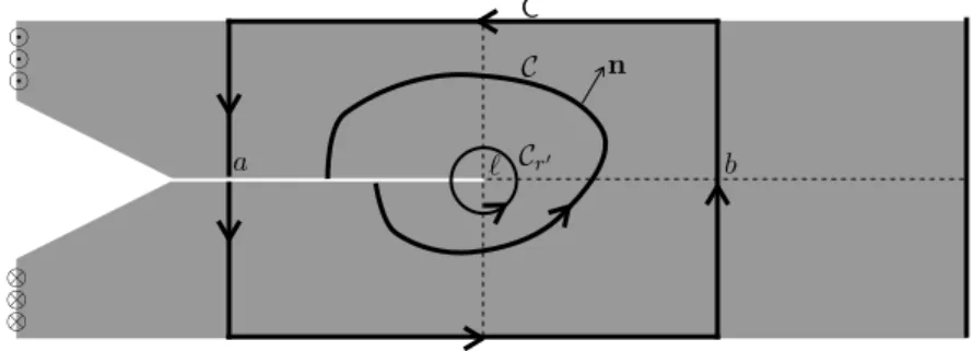
Figure 5. Examples of paths for which)#is equal to&l.

length of the crack:

&l = d3l

dl . (53)

Even though3l involves the l-dependent displacement field ul, its derivative does

not involve the derivative dul/dl but can be expressed in terms of ul only. This

property is a consequence of the fact that ul satisfies the equilibrium equations.

Specifically,&lcan be computed either with the help of path integrals like the)

inte-gral of [Rice 1968] or by using the so-called G-✓ method developed in [Destuynder and Djaoua 1981]. We recall below the main ingredients of both methods when 0 < l < L. The cases l = 0 and l = L are treated separately.

In the former method, the integral)# over the path#is defined by

)#= Z # ✓_µ 2 rul· ruln1 µ @ul @n @ul @x1 ◆ ds,

wheren denotes the outer normal of the path. This integral is (theoretically) path-independent and equal to&_l provided that the path# starts from the lip of the crack, circumvents the tip of the crack and finishes on the lip of the crack like in Figure 5; see [Bui 1978]. This path independence is used to obtain Irwin’s formula [Irwin 1958; Leblond 2003]. Indeed, taking for path the circle#r0 centered at the

tip of the crack with radius r0_{, using (50) and passing to the limit when r}0_{! 0,}

the following link between the energy release rate and the stress intensity factor Kl introduced in (50) is obtained: &l = lim r0_!0)#r0 = K2 l 2µ.

For the computations, the particularities of the geometry and of the loading can be exploited, to choose a path made of line segments parallel to the axes like the path

Cin Figure 5:

with 0 < a < l < b < L. Then)C=&l. Therefore, since n1= 0 and @ul/@n = 0

on the sides x2= ±H and by virtue of the symmetry of ul,&l takes the form

&_{l = µ} Z {b}⇥(0,H) ✓✓ @ul @x2 ◆2 ✓ @ul @x1 ◆2◆ dx2 µ Z {a}⇥(0,H) ✓✓ @ul @x2 ◆2 ✓ @ul @x1 ◆2◆ dx2. (54)

From a theoretical point of view, a and b can be chosen arbitrarily, provided that they satisfy the constraints above. Indeed, the integral over the line segment x1= a

(respectively, x1= b) does not depend on a (respectively, on b) because ul is

har-monic and satisfies homogeneous Neumann boundary conditions on N± _{and 0l.}

(This verification is left to the reader; see [Marigo 2010, Proposition 8] for a proof.) However, from a numerical point of view, this is no longer true because the computed displacement field does not satisfy exactly the equilibrium equations. Consequently, the computed values of&l depend on the choice of a and b.

More-over, since the integral over the line a involves the gradient of the displacement, this integral can be badly approximated when l is small because of the singularity. The G-✓ method is based on a change of variables which sends the l-dependent domain l onto a fixed domain. In essence, it is the basic method to prove that

l 7!3l is differentiable; see [Destuynder and Djaoua 1981] for the genesis of this

method and [Chambolle et al. 2010] for a discussion on a generalization of the concept of energy release rate. In turn the G-✓ approach gives a practical method to compute the energy release rate; see the previous two references. Specifically, for a given l > 0, we associate to a Lipschitz continuous vector field ✓ defined on l the volume integral

G✓ = Z l ✓ ₂ P i, j=1µ @✓i @xj @ul @xi @ul @xj µ 2 rul· ruldiv ✓ ◆ dx.

It can shown that, if ✓ is such that ✓(l, 0) = e1 and ✓ · n = 0 on @l, thenG✓ is

independent of ✓ and equal to&l. Of course, this result of independence holds only

when ul is the true displacement field. If it is numerically approximated, thenG✓

becomes ✓ dependent. In our case, owing to the simplicity of the geometry, we can use a very simple vector field ✓ which renders the computations easier. Specifically, let ✓ be given by ✓ (x) = 8 > > > > < > > > > : 0 if x1<0, x1 l e1 if 0  x1 l, L x1 L l e1 if l  x1<L. (55)

It satisfies the required conditions and henceG✓ =&l. Accordingly, owing to the

symmetry,&_l takes the form

&l = µ L l Z L l Z H 0 ✓✓ @ul @x2 ◆2 ✓_@u l @x1 ◆2◆ dx2dx1 µ l Z l 0 Z H 0 ✓✓ @ul @x2 ◆2 ✓_@u l @x1 ◆2◆ dx2dx1. (56) Comparing (56) with (54), (56) can be seen as an average of all the line integrals appearing in (54) when a and b vary, respectively, from 0 to l and from l to L. Accordingly, it can be expected that (56) gives more accurate computations than (54) when l is small.

3.3. Numerical results obtained for&_l by the FEM. All the computations based

on the finite element method are implemented in the industrial code COMSOL. They are performed after introducing dimensionless quantities. Specifically, in all the computations, the dimensions of the body are H = 1 and L = 5, the shear modulus µ = 1. That does not restrict the generality of the study because the scale dependencies are known in advance. Indeed, the true physical quantities are related to the normalized quantities (denoted with a tilde) by

l = H ˜l, ul= H ˜ul, 3l= µH23˜l, &l= µH ˜&l. (57)

For a given ˜l2 (0, 5) and a given ✏ 2 (0, 1), we use the symmetry of the body and of the load to mesh only its upper half and prescribe ˜ul= 0 on the segment ˜l  ˜x1 5,

˜x2= 0. We use 6-node triangular elements, i.e., quadratic Lagrange interpolations.

The mesh is refined near the singular corners and a typical mesh contains 25000 el-ements and 50000 degrees of freedom. We compute the discretized solution (still denoted) ˜ul by solving the linear system. Then, the energy ˜3l and the energy

release rate ˜&l are obtained by postprocessing. The energy is obtained by a direct

integration of the elastic energy density over the body. The derivative of the energy is obtained by using formula (56), which needs to integrate the different parts of the elastic energy density over the two rectangles (0, ˜l) ⇥ (0, 1) and (˜l, 5) ⇥ (0, 1). For a given ✏, we compute ˜3_l and ˜&_l for ˜l varying from 0.001 to 5, first by steps of 0.001 in the interval (0, 0.05), then by steps of 0.002 in the interval (0.05, 0.2), finally by steps of 0.01 in the interval (0.2, 5). The computations can be considered sufficiently accurate for ˜l 0.002, even if this lower bound depends on ✏, the computations being less accurate for small (but nonzero) values of ✏. Below this value, if we try to refine the mesh near the corner of the notch, the results become mesh-sensitive, and the linear system becomes ill-conditioned. Since only the part of the graph of ˜&l close to ˜l = 0 is interesting when ✏ is small, we cannot obtain

0 0.1 0.2 0.3 0.4 0.5 0 1 2 3 4 5 &l µH l/H ✏= 0.0 ✏= 0.1 ✏= 0.2 ✏= 0.3 ✏= 0.4

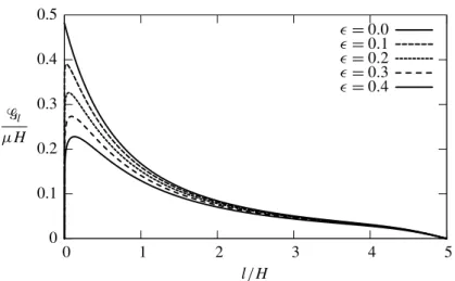
Figure 6. Computation by the Finite Element Method of the en-ergy release rate &l as a function of the crack length l for five

values of the notch angle.

accurate results when ✏ is too small. (Of course, this remark does not apply when ✏= 0, because ˜l = 0 is not a “singular” case.)

The cases ˜l = 0 and ˜l = 5 with ✏ 6= 0 are treated with specific meshes. We have only to compute ˜u0, ˜30, ˜uL and ˜3L, since ˜&0= ˜&L= 0.

The case ✏ = 0 is treated separately by adapting the previous methods. In par-ticular, to calculate ˜&l, the second integral in (56) is replaced by an integral over

the rectangle ( 1, 0) ⇥ (0, 1), and this integral is divided by 1 + ˜l instead of ˜l. Moreover, the mesh is refined only near the tip of the crack; ˜l = 0 is no longer a particular case and the computations of ˜&l are accurate in the full range of ˜l.

Let us highlight the main features of the numerical results plotted in Figure 6. These properties will be the basic assumptions from which we study the crack propagation at the end of the present section.

(P1) For ✏ = 0,&_l/µH is monotonically decreasing from 0.4820 to 0 when l/H grows from 0 to 5.

(P2) For ✏ > 0,&l/µH starts from 0 at l/H = 0, then is rapidly increasing. This

growth is of such magnitude (for instance,&l/µH = 0.1443 when l/H =

0.002 for ✏ = 0.4) that it cannot be correctly captured by the FEM.

(P3) Still for ✏ > 0,&l is monotonically increasing as long as l  lm. At l = lm,&

takes its maximal valueGm. Those values which depend on ✏ are given in the

✏ 0 0.1 0.2 0.3 0.4

lm/H 0 0.024 0.058 0.092 0.130

Gm/µH 0.4820 0.3900 0.3260 0.2733 0.2279

(P4) For ✏ > 0 again,&_l is monotonically decreasing fromGmto 0 when l grows

from lmto 5H.

3.4. Evaluation of the energy release rate by the MAM. By virtue of (52),3l can

be expanded by using the outer expansion of ul. Using (47) leads to

3l=X i2N P2i✓ l H ◆2i µH2, (58)

where the coefficients P2i of the expansions are dimensionless. The expansion of

the energy release rate can be immediately deduced from that of the energy:

&_{l =} X i2N⇤ 2i P2i✓ l H ◆2i 1 µH, (59)

and it is not necessary to use the path integrals )# or the G-✓ method. Let us

remark that

&0=

⇢

0 if ✏ 6= 0,

P2µH = K₀2/2 > 0 if ✏ = 0, (60) because > 1/2 in the former case while = 1/2 in the latter.

To obtain the i-th term of the expansion of3l and&l, both the singular part ui_S

and the regular part ¯ui _{of u}i _{must be recovered. The singular part involves the}

coefficientsai_nfor 1  n  i which are obtained as the regular parts of the vj for

j  i; see Section 2.2.6. Therefore, the inner problems must be solved to determine the coefficientsbi_n for 0  n  i. In practice, these coefficients are obtained by

using Proposition 4 after the inner and the outer problems have been solved with a finite element method. The advantage is that those problems do not contain a small defect and the accuracy is guaranteed. The drawback is that more and more problems have to be solved, in order to obtain accurate values of&l when l/H is

not small.

In Tables 3 and 4 are given the computed values of the first coefficients of the inner and outer expansions (still with H = 1, L = 5, µ = 1). These tables contain all the terms which are necessary to compute the expansions of the energy up to the sixth order, i.e., P2i for i 2 {0, 1, 2, 3}. (Note that P0does not appear in the

expansion of&l.) The graphs of l 7!&l obtained from these expansions are plotted

in Figure 7 in the cases ✏ = 0.2 and ✏ = 0.4. They are compared with the values obtained directly by the finite element code COMSOL. From these comparisons, the following conclusions can be drawn:

✏ a2₁ P2 0 0.3930 0.4820 0.1 0.3756 0.4413 0.2 0.3559 0.3957 0.3 0.3342 0.3486 0.4 0.3106 0.3005 a4₁ a4₃ P4 0.1888 0.0987 0.3282 0.1766 0.0943 0.3001 0.1619 0.0893 0.2673 0.1453 0.0838 0.2320 0.1273 0.0778 0.1952 a6₁ a6₃ a6₅ P6 0.1365 0.0537 0.0494 0.2013 0.1279 0.0507 0.0472 0.1931 0.1165 0.0470 0.0446 0.1787 0.1029 0.0427 0.0418 0.1603 0.0880 0.0380 0.0389 0.1385

Table 3. The computed values of the (nonzero) coefficientsai_n for

1  n  i  6 and of the leading terms P2, P4 and P6 of the

expansion of the potential energy for several values of the angle of the notch. ✏ b1₁ b3₁ b3₃ 0 0.7834 0.2384 0.2059 0.1 0.7482 0.2091 0.2085 0.2 0.7089 0.1777 0.2081 0.3 0.6657 0.1451 0.2045 0.4 0.6187 0.1125 0.1977 b5₁ b5₃ b5₅ 0.1943 0.1058 0.0172 0.1730 0.0992 0.0283 0.1489 0.0905 0.0379 0.1232 0.0800 0.0454 0.0974 0.0683 0.0508

Table 4. The computed values of the (nonzero) coefficientsbi_n for

1  n  i  5 for several values of the angle of the notch.

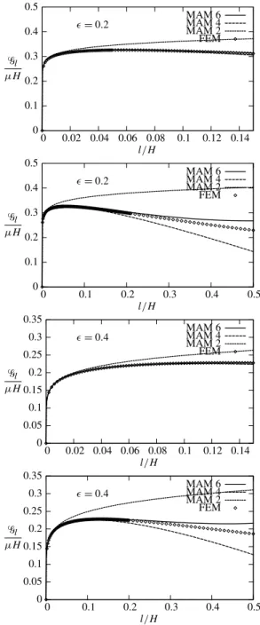
(C1) For very small values of l, the first nontrivial term (corresponding to i = 1 in (59)) of the matched asymptotic expansion (denoted by MAM 2 in Figure 7) is sufficient to well approximate&_l while the FEM is unable to deliver accu-rate values.

(C2) For values of l of the order of lm, at least the first two nontrivial terms

(corre-sponding to i = 1 and 2 in (59)) of the MAE (denoted by MAM 4 in Figure 7) are necessary to capture the change of monotonicity of&l. Indeed, the first

term, being monotonically increasing, is unable, alone, to capture that change of behavior.

(C3) Still for values of l of the order of lm, the first two terms are really sufficient

to well approximate&l provided that lm/H is sufficiently small. Specifically,

the first two terms are sufficient as long as l/H < 0.2.

(C4) Accordingly, the approximation of&l by the first two nontrivial terms of the

MAE can be used, in the range [0, 2lm] of l when ✏ 2 (0, 0.4).

(C5) As l/H grows beyond 0.2, more and more terms of the MAE must be added, in order to get a good approximation of&l. Consequently, in the range of

“large” values of l/H, the direct FEM is more accurate and hence is better to use.

4. Application to the determination of the nucleation of the crack The theoretical and numerical results obtained in the previous sections are used here to study the delicate issue of the nucleation of a crack in a sound body or the most classical question of the onset of a preexisting crack. Specifically, we consider the notched body 0which either contains a preexisting crack l0>0 or is

sound; i.e., l0= 0. We have also to distinguish different cases according to whether

✏= 0 or ✏ > 0. The nucleation or the onset of cracking is governed by either the so-called G-law or the so-called FM-law and one goal of this section is to compare those laws. The interested reader can also refer to [Bourdin et al. 2008; Francfort and Marigo 1998; Negri 2010; Negri and Ortner 2008; Marigo 2010] where other comparisons between the G-law and the FM-law are proposed.

The notched body is submitted to a time-dependent loading process which con-sists of a monotonically increasing amplitude of the displacement prescribed on the sides D±_{. Specifically, consider the new boundary conditions}

u = ±t H on D±, t 0. (61)

The others remain unchanged. (Note that the “time” parameter t is dimensionless.) The evolution problem consists of finding the time evolution of the length of the crack, i.e., t 7! l(t) for t 0, under the initial condition l(0) = l02 [0, L). For

that, we first remark that, for a given time t 0 and a given crack length l 2 [0, L], the displacement field which equilibrates the body is

u(t, l) = tul, (62)

where ul is the displacement field introduced in Section 3.1. Accordingly, the

potential energy and the energy release rate at time t with a crack length l can be expressed as

3(t, l) = t23_l, &(t, l) = t2&_l, (63) where3l and&l are given by (51) and (53).

The two evolution laws are based on Griffith’s crucial assumption [1921] con-cerning the surface energy associated with a crack. Specifically, assume that there exists a material constantGc>0 such that the surface energy of the body with a

crack of length l is

✏_{= 0.2} 0 0.1 0.2 0.3 0.4 0.5 0 0.02 0.04 0.06 0.08 0.1 0.12 0.14 &l µH l/H MAM 6 MAM 4 MAM 2 FEM ✏_{= 0.2} 0 0.1 0.2 0.3 0.4 0.5 0 0.1 0.2 0.3 0.4 0.5 &l µH l/H MAM 6 MAM 4 MAM 2 FEM ✏= 0.4 0 0.05 0.1 0.15 0.2 0.25 0.3 0.35 0 0.02 0.04 0.06 0.08 0.1 0.12 0.14 &l µH l/H MAM 6 MAM 4 MAM 2 FEM ✏= 0.4 0 0.05 0.1 0.15 0.2 0.25 0.3 0.35 0 0.1 0.2 0.3 0.4 0.5 &_l µH l/H MAM 6 MAM 4 MAM 2_FEM

Figure 7. Comparison of the graphs of&_l obtained by the MAM and by COMSOL for ✏ = 0.2 (top two plots) and ✏ = 0.4 (bottom two). The curve labeled FEM indicates points obtained by COM-SOL, while the curves labeled MAM 2i, i 2 {1, 2, 3}, indicate that the first i nontrivial terms in the expansion of&l were considered.

Accordingly, the total energy of the body at equilibrium at time t with a crack of length l becomes

%(t, l) :=3(t, l) +6(l) = t23l+Gcl. (65)

Throughout this section we assume that l 7!3l is continuously differentiable and

monotonically decreasing. Moreover, some monotonic properties of l 7!&l will

be added when necessary according to the analysis made in the previous sections. 4.1. The two evolution laws. Let us briefly introduce the two evolution laws; the reader interested in the details should refer to [Marigo 2010]. The first one, called the G-law, is the usual Griffith law based on the critical potential energy release rate criterion; see [Bui 1978; Leblond 2003; Nguyen 2000]. In essence, this law only investigates smooth (i.e., at least continuous) evolutions of the crack length with the loading. It consists of the three following items:

Definition 2 (G-law). Let l02 [0, L]. A continuous function t 7! l(t) is said to

satisfy (or to be a solution of) the G-law in the interval [t0,t1] with the initial

condition l(t0)= l0, if the three following properties hold:

(1) Irreversibility: t 7! l(t) is not decreasing;

(2) Energy release rate criterion: &(t, l(t)) Gc for all t 2 [t0,t1];

(3) Energy balance: l(t) is increasing only if&(t, l(t)) =Gc; i.e., if&(t, l(t)) <

Gc at some t, then l(t0)= l(t) for every t0 in a certain neighborhood [t, t + h)

of t.

The third item implies that the release of potential energy is equal to the cre-ated surface energy when the crack propagates, which justifies its name “energy balance”. Consequently, if t 7! l(t) is absolutely continuous, then the third item is equivalent to

@%

@l(t, l(t))˙l(t) = 0

for almost all t, and the following equality holds for almost all t: d

dt%(t, l(t)) = @%

@t(t, l(t)). (66)

A major drawback of the G-law is the inability to take into account discontinuous crack evolutions, which renders it useless in many situations as we will see in the next subsection. It must be replaced by another law which admits discontinuous solutions. Another motivation of changing the G-law is to reinforce the second item by introducing a full stability criterion; see [Francfort and Marigo 1998; Nguyen 2000; Bourdin et al. 2008]. Specifically, let us consider the local stability condition 8t 0, 9h(t) > 0 : %(t, l(t)) %(t, l) 8l 2 [l(t), l(t) + h(t)], (67)

which requires that the total energy at t is a “unilateral” local minimum. (The qual-ifier unilateral is added because the irreversibility condition leads to comparing the energy at t with only that corresponding to greater crack length; see [Bourdin et al. 2008].) Taking l = l(t)+h with h > 0 in (67), dividing by h and passing to the limit when h ! 0, we recover the critical energy release rate criterion. Thus, the second item can be seen as a first-order stability condition, weaker than (67). A stronger requirement is obtained by replacing local minimality by global minimality. It was the condition introduced in [Francfort and Marigo 1998] in the spirit of the original Griffith idea [1921], and we will adopt it here.

Definition 3 (FM-law). A function t 7! l(t) (defined for t 0 and with values in [0, L]) is said to satisfy (or to be a solution of) the FM-law if the three following properties hold:

(1) Irreversibility: t 7! l(t) is not decreasing;

(2) Global stability: %(t, l(t)) %(t, l) for all t 0 and all l 2 [l(t), L]; (3) Energy balance:%(t, l(t)) =%(0, l0)+R₀t@%/@t0(t0,l(t0))dt0 for all t 0.

Let us note that the irreversibility condition is unchanged, while the energy balance condition is now written as the integrated form of (66), which does not require that t 7! l(t) be continuous. Note also that the energy balance implies l(0) = l0because 0 =%(0, l(0)) %(0, l0)=Gc(l(0) l0), and that the second item

is automatically satisfied at t = 0 because%(0, l) =Gcl.

4.2. The main properties of the G-law and the FM-law. We recall or establish in this subsection some results for the two evolution laws under the assumptions of monotonicity of l 7!&l resulting from the numerical computations; see (P1)–

(P4) in Section 3.3. Some of those results have a general character and have been previously established in [Bourdin et al. 2008; Francfort and Marigo 1998; Marigo 2010], while the other ones are specific to the present problem. In the case of properties which have already been obtained, we simply recall them without proofs.

Let us first consider the case when the notch is in fact a crack. Then, the two laws are equivalent by virtue of:

Proposition 5. In the case ✏ = 0, since l 7!&lis decreasing from&0>0 to 0 when l goes from 0 to L (see property (P1)), the G-law and the FM-law admit the same unique solution. Specifically, the preexisting crack begins to propagate at timeti

such thatti2&l0=Gc. Then the crack propagates continuously and l(t) is such that

t2_&

l(t)=Gc. Since&L= 0, the crack will not reach the end L in a finite time.

Proof. See [Marigo 2010, Proposition 18]. ⇤

In the case of a genuine notch, as far as the nucleation and the propagation of a crack with the G-law are concerned, we have:

Proposition 6. In the case ✏ > 0, according to l0= 0 or l02 (0, lm)or l02 [lm,L),

the crack evolution predicted by the G-law is as follows:

(1) If l0= 0, since&0= 0, the unique solution to the G-law is l(t) = 0 for all t;

i.e., there is no crack nucleation.

(2) If l02 (0, lm), then the preexisting crack begins to propagate at timeti such

thatti2&l0 =Gc. But atti the propagation is necessarily discontinuous and

hence there is no continuous solution to the G-law for t ti.

(3) If l02 [lm,L), since l 7!&l is monotonically decreasing in the interval (lm,L),

the situation is the same as in Proposition 5. There exists a unique solution for the G-law: the crack begins to propagate atti(still given byti2&l0=Gc)

and then propagates continuously until L, which is reached asymptotically. Proof. Let us give the sketch of the proof for the first two items.

(1) Since l0= 0 and&0= 0, then for all t 0 one gets 0 =&(t, 0) <Gcand hence

l(t) = 0 is a solution. The uniqueness follows from the initial condition and the energy balance.

(2) Since 0 < l0<lm, then&l0 >0 and hence t2&l0=&(t, l0)Gc if and only if

t 2 [0,ti]. Since the inequality is strict when t 2 [0,ti), then l(t) = 0 is the

unique solution in this interval because of the initial condition and the energy balance. By continuity, it is also the unique solution in the closed interval [0,ti]. On the other hand, since &(t, l0) >Gc when t > ti, the crack must

begin to propagate atti.

Let us show that no (continuous) evolution can satisfy the G-law for t >ti.

Indeed, by construction&(ti,l(ti))=ti2&l0 =Gc. But since l(t) lifor t >ti

and since l 7!&l is monotonically increasing in the neighborhood of l0<lm,

we have for t 2 (ti,ti+ h) and a sufficiently small h > 0:

l0<l(t) < lm, &(t, l(t)) >&(ti,l0)=Gc.

Therefore the energy release rate criterion cannot be satisfied by a continuous evolution in a neighborhood ofti. The unique possibility is that the length of

the crack jumps from l0to some li>lmat timeti. But that requires

reformu-lating the G-law.

The proof of the third item is the same as in the previous proposition and hence

we refer to [Marigo 2010, Proposition 18]. ⇤

Remark 8. This property of no nucleation of a crack at a notch or of brutal prop-agation of a short crack is due to the fact that a notch with Neumann boundary conditions induces a weak singularity only; i.e., > 1/2. If one changes the boundary conditions by imposing the displacement on one edge of the notch and the stress on the other edge, then the singularity becomes strong for ! large enough

and in such a case all the properties of nucleation are changed; see [Francfort and Marigo 1998, Proposition 4.19].

Consider now the FM-law. It is proved in [Marigo 2010, Proposition 3] that, in the case of a monotonically increasing loading, the FM-law is equivalent to a minimization problem of the total energy at each time, as precisely stated in the following lemma:

Lemma 7. Let l02 [0, L) be the initial length of the crack. A function t 7! l(t)

satisfies the FM-law if and only if , at each t, l(t) is a minimizer of l 7!%(t, l) over [l0,L]. Therefore, the FM-law admits at least one solution and each solution

grows from l0to L.

This property holds true for any ✏ 0. In the case ✏ > 0 we can deduce precise results:

Proposition 8. In the case ✏ > 0, according to l02 [0, lm)or l02 [lm,L), the crack

evolution predicted by the FM-law is as follows:

(1) If l02 [0, lm), then the nucleation (if l0= 0) or the propagation of the

preexist-ing crack (if l06= 0) starts at timeti>0 and at this time the crack length jumps

instantaneously from l0to li. The length liis the unique length in (lm,L) such

that Z li

l0

&ldl = (li l0)&li, or, equivalently, 3l0 3li= (li l0)&li, (68)

while the timetiis given by

ti2&li =Gc. (69)

After this jump, the crack propagates continuously from lito L, the evolution

satisfying then the G-law; i.e., t2_&

l(t)=Gc for all t >ti.

(2) If l02 [lm,L), since l 7!&l is monotonically decreasing in the interval (lm,L),

the situation is the same as in Proposition 5. There exists a unique solution for the FM-law which is the same as for the G-law: the crack begins to propagate attisuch thatti2&l0=Gcand then propagates continuously until L, which is

reached asymptotically.

Remark 9. Before the proof of this proposition, let us comment and interpret (68) giving the jump of the crack atti.

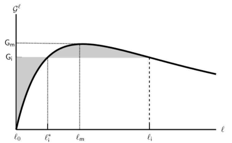
i i Gi G Gm m 0

Figure 8. Graphical interpretation of the criterion of crack nucle-ation given by the FM-law and which obeys the Maxwell rule of equal areas.

• Let us first prove that liis well defined by (68). Let l 7! g(l) be the function

defined for l 2 (lm,L) by

g(l) = Z l

l0

&ldl (l l0)&l. Its derivative is given by g0_{(l) = (l l0)&}0

l and hence is positive because&l

is decreasing in (lm,L). Since&l <Gm:=&lm, g(lm) <0, whereas g(L) > 0

because&L= 0. Therefore, there exists a unique l 2 (lm,L) such that g(l) = 0,

what is precisely the definition of li.

• Equation (68) giving lihas a graphical interpretation. Indeed, the integral over

(l0,li)represents the area under the graph of l 7!&l between the lengths l0

and li. On the other hand the product (li l0)&li represents the area of the

rectangle whose height isGi:=&li. Therefore, since these two areas are equal,

the two gray areas of Figure 8 are also equal. This rule of equality of the areas determines li and, by essence, the line&=Giis the classical Maxwell line

which appears in any problem of minimization of a nonconvex function.

• Note that li is independent of the toughnessGc and of the shear modulus µ

of the material. It is a characteristic of the structure and merely depends on the geometry and the type of loading. Here, it depends on ✏, H and L. For a given ✏ and a given ratio L/H, liis proportional to H, li= ˜liH. This property

is a consequence of the Griffith assumption on the surface energy.

• The critical loading amplitudetidepends on the toughness and on the size of

the body. Since&li = ˜&liµH,tivaries like 1/

p

H. This size effect is also a consequence of the Griffith assumption on the surface energy.

• By virtue of (68) and (69), the energy balance holds at timeti even if the

crack jumps at this time; i.e., the total energy of the body just before the jump is equal to the total energy just after. Indeed, those energies are respectively given by

%(ti ,l0)=ti23l0+Gcl0, %(ti+, li)=ti23li+Gcli.

Using (68), (69) and the equality 3l0 3li =

Rli

l0&ldl, then %(ti ,l0) = %(ti+, li).

Proof of Proposition 8. We just prove the first part of the proposition and the reader should refer to [Marigo 2010, Proposition 18] for the proof of the second part. Let l02 [0, lm). By virtue of Lemma 7, l(t) is a minimizer of l 7!%(t, l) over [l0,L].

(The minimum exists because the energy is continuous and the interval is compact.) Let li,tibe given by (68)–(69), letGi=&li and let li⇤be the other length such that

&l⇤

i =Gi; see Figure 8. Let us first remark that the function l 7! ¯g(l) defined on

[l0,L] by

¯g(l) :=Gi(l l0) (3l0 3l)

is nonnegative and vanishes only at l0and li. Indeed, its derivative is ¯g0(l) =Gi &l.

Hence, ¯g is first increasing from 0 when l grows from l0to l⇤i, then decreasing to 0

when l grows from l⇤

i to li, and finally increasing again from 0 when l grows from

lito L.

Let us show that l0is the unique minimizer of the total energy when t <ti. From

(68) and (69), we get for all l 2 [l0,L] and all t ti:

%(t, l) %(t, l0)= t2(3l0 3l)+Gc(l l0) t2¯g(l) 0.

Moreover, the inequalities above are equalities if and only if l = l0when t <tiand

the result follows. Using the same estimates, we can deduce that l0and liare the

two minimizers of the total energy at t =ti.

Let us show now that the minimizer is in the open interval (li,L) when t >ti.

From (68) and (69), we get for all l 2 [l0,li)and all t >ti:

%(t, l) %(t, li)= t2(3l 3li) Gc(li l) >ti

2 ₃

l 3li Gi(li l)

=ti2 ¯g(l) ¯g(li) =ti2¯g(l) 0.

Hence, the minimizer cannot be in [l0,li). Since the derivative of the total energy

at l = liis equal toGc t2Gi<0, liis not the minimizer. In the same manner, since

the derivative of the total energy at l = L is equal toGc t2&L=Gc>0, L cannot

be the minimizer. Therefore, the minimizer is in the interval (li,L) when t >ti.

Hence, it must be such that the derivative of the total energy vanishes, which yields t2_&