Miocene climate modelling sensitivity experiments for different CO2 concentrations

http://palaeo-electronica.org

PE Article Number: 12.2.5A

Copyright: Palaeontological Association August 2009 Submission: 9 October 2008. Acceptance: 28 April 2009

Micheels, Arne, Bruch, Angela A., and Mosbrugger, Volker, 2009. Miocene Climate Modelling Sensitivity Experiments for Different CO₂ Concentrations. Palaeontologia Electronica Vol. 12, Issue 2; 5A: 20p;

MIOCENE CLIMATE MODELLING SENSITIVITY EXPERIMENTS

FOR DIFFERENT CO

₂

CONCENTRATIONS

Arne Micheels, Angela Bruch, and Volker Mosbrugger

ABSTRACT

Throughout the Cenozoic the global climate cooled, but until the Pliocene, tem-peratures in polar regions seem to have been higher than at present, and it is not yet clear if the Arctic Ocean was already ice-covered in the Miocene. Reconstructions for Miocene atmospheric carbon dioxide concentration do not give a coherent climatic pic-ture: intervals of ice-free conditions in the Arctic region appear to correspond to low CO₂, and intervals during which the Arctic Ocean was ice-covered had high CO₂ lev-els. Here we present the results of climate modelling sensitivity experiments for the Late Miocene, considering different CO2 concentrations. In order to get ice-free condi-tions in the Arctic Ocean, a CO2 concentration of at least 1500 ppm is necessary. Con-centrations this high are unlikely for the Miocene, and our results support onset of Northern Hemisphere glaciation earlier than Late Miocene. Compared to future climate change scenarios with enhanced CO2, the modelled temperature response to CO2 increase is slightly weaker in our Miocene sensitivity experiments. This dampened response is due to the decreased sea ice volume in the Miocene and the reduced ice-albedo feedback. Comparing our sensitivity experiments with quantitative terrestrial proxy data to give an estimation for pCO₂ in the Late Miocene we find that model runs with 360 ppm and 460 ppm are most consistent with proxy data. This validation thus suggests that Late Miocene CO2 concentrations were higher than present but lower than 500 ppm.

KEYWORDS: Miocene, Late; climate modelling; sensitivity experiment; CO2; proxy data comparison Arne Micheels. Senckenberg Forschungsinstitut und Naturmuseum, Biodiversität und Klima Forschun-gszentrum (LOEWE BiK-F), Senckenberganlage 25, D-60325 Frankfurt/Main, Germany. arne.micheels@senckenberg.de.

Angela Bruch. Forschungsstelle "The role of culture in early expansions of humans“ der Heidelberger Akademie der Wissenschaften, Senckenberg Forschungsinstitut und Naturmuseum, Senckenberganlage 25, D-60325 Frankfurt/Main, Germany. angela.bruch@senckenberg.de.

Volker Mosbrugger. Senckenberg Forschungsinstitut und Naturmuseum, Biodiversität und Klima Forsc-hungszentrum (LOEWE BiK-F), Senckenberganlage 25, D-60325 Frankfurt/Main, Germany. volker.mos-brugger@senckenberg.de.

INTRODUCTION

The Miocene (~ 23 to 5 Ma) was part of the general late phase of Cenozoic cooling, but its cli-mate was still a general hothouse situation. Vari-ous proxy data suggest it had a warmer and more humid climate than today (e.g., Wolfe et al. 1994a,b; Zachos et al. 2001; Bruch et al. 2004, 2006, 2007; Mosbrugger et al. 2005). In particular, the Miocene equator-to-pole latitudinal tempera-ture gradient was weak, implying that higher lati-tudes were warmer than they are today (e.g., Wolfe 1994a,b; Bruch et al. 2004, 2006, 2007). Corre-sponding to warm polar regions during the Mio-cene, it was commonly assumed that the large-scale glaciation of the Northern Hemisphere did not start until the latest Miocene or the Pliocene (e.g., Kleiven et al. 2002; Winkler et al. 2002; Bar-toli et al. 2005; St. John and Krissek 2002). How-ever, some studies have raised questions about when significant Arctic sea ice first formed (e.g., Helland and Holmes 1997; Moran et al. 2006). It remains an open debate when sea ice first appeared in the Northern Hemisphere, although most recent evidences seems to support that the Arctic Ocean was already ice-covered in the Mio-cene (e.g., Moran et al. 2006). If so, polar regions in the Miocene may have been cooler than hereto-fore assumed.

Increasing carbon dioxide in the atmosphere is the primary agent for future climate change (e.g., Cubasch et al. 2001; Meehl et al. 2007). Thus, the amount of atmospheric CO₂ in the Miocene is rele-vant to the question of what palaeotemperatures were then. Some studies suggest that the Miocene CO2 level was close to the pre-industrial concen-tration (280 ppm) or a little higher (e.g., Pearson and Palmer 2000; Pagani et al. 2005). However, other studies support a pCO2 being as high as 500 ppm (e.g., MacFadden 2005) to 700 ppm (e.g., Cerling 1991). Retallack (2001) even proposed that atmospheric carbon dioxide was higher than 1000 ppm until the Late Miocene. It is difficult to con-ceive that high latitudes would have been warm if CO2 was low in the Miocene, but it also seems improbable that polar regions were ice-covered if CO₂ concentrations were high.

Previous climate model experiments for the late Tertiary concentrated primarily on either the roles of geography and orography (e.g., Ramstein et al. 1997; Ruddiman et al. 1997; Kutzbach and

Behling 2004) or on the role of the ocean (e.g., Bice et al. 2000; Steppuhn et al. 2006) as a major influence on climate. In order to adapt their models to Miocene conditions, modellers must specify the concentration of atmospheric CO₂; however the fact that the Miocene CO2 level is still debated, cli-mate models of Miocene time intervals are quite variable (e.g., Kutzbach and Behling 2004; Step-puhn et al. 2006, 2007). Recently, StepStep-puhn et al. (2007) presented a sensitivity experiment for the Late Miocene, which analysed the effects of using a concentration of 2×CO2 (700 ppm) as compared to 1×CO₂ (353 ppm). Even with 700 ppm, the Late Miocene model experiments indicated that the Arc-tic Ocean would still have been ice-covered (Step-puhn et al. 2007), results which appear to conflict with the fossil record. Furthermore, the heating of high latitudes in these high-CO₂ model experi-ments occurred at the expense of warming lower latitudes, which conflicts with proxy data (Steppuhn et al. 2007). Steppuhn et al. (2007) concluded that while high CO2 did not explain warm high latitudes, palaeovegetation might. Miocene vegetation is indeed thought to have contributed to warm high latitudes (Dutton and Barron 1997; Micheels et al. 2007), but climate modellers still run into trouble when trying to understand warm high latitudes in the Miocene (Steppuhn et al. 2006, 2007; Micheels et al. 2007). A low atmospheric pCO2 is not suffi-cient to explain the warm Miocene climate, nor does a high concentration explain the distribution of temperatures (Steppuhn et al. 2007; Micheels et al. 2007). But what if CO₂ was intermediate?

Geological processes such as the mountain uplift from the Miocene until today and their influ-ence on climate had repeatedly attracted the inter-est for model experiments (e.g., Ramstein et al. 1997). In contrast, sensitivity experiments with respect to CO₂ are rare (Steppuhn et al. 2007; Tong et al. 2009). Levels of carbon dioxide in the Miocene are not known for sure (e.g. Retallack 2001; Pagani et al. 2005), but realistic model experiments specifically require CO2 levels to be properly specified. Climate models are tools to test hypotheses and to understand specific processes – carbon dioxide is a general key factor for climate (e.g., Meehl et al. 2007), but in terms of Tertiary cli-mate modelling the relevance of carbon dioxide is poorly understood. This situation is unsatisfying since the Miocene could serve as a possible

ana-logue for the future climate change if it were better understood (e.g., Kutzbach and Behling 2004). Three basic points still remain open for discussion: 1. How high must atmospheric CO2 be so that

the Arctic Ocean is ice-free in the Miocene? 2. What was the general climate sensitivity o

enhanced pCO2 in the Miocene? Is the Late Miocene comparable to future climate change scenarios?

3. How consistent are different Late Miocene CO₂ scenarios compared to proxy data? Can we estimate a Late Miocene pCO2 from com-paring models and independent proxy data? To address these questions, we perform sen-sitivity experiments for the Late Miocene using an earth system model of intermediate complexity Planet Simulator. Based on a reference run, we present sensitivity experiments that consider pCO₂ values ranging from low (200 ppm) to high (700 ppm). In addition, we perform a transitional experi-ment with a steady increase of CO₂ by +1 ppm starting with 200 ppm and ending up with 2000 ppm. Finally, we use quantitative terrestrial proxy data to validate the model results. The results of our sensitivity experiments contribute to a better understanding of the role of CO2 for the Cenozoic climate history.

THE MODEL AND EXPERIMENTAL SETUP The Planet Simulator

In order to perform our sensitivity experi-ments, we used an earth system model of interme-diate complexity (EMIC) Planet Simulator (Fraedrich et al. 2005a,b). The spectral atmo-spheric general circulation model (AGCM) PUMA-2 is the core module of the Planet Simulator. The model has a horizontal resolution of T21 (5.6° × 5.6°). Five layers represent the vertical domain using terrain-following sigma-coordinates. The atmosphere model is an advanced version (e.g., including moisture in the atmosphere) of the simple AGCM PUMA (e.g., Fraedrich et al. 1998). As com-pared to the first ‘dry-dynamics version’, the atmo-sphere module now includes schemes for physical processes such as radiation transfer, large-scale and convective precipitation, and cloud formation. The atmosphere model is coupled to a slab ocean and a thermodynamic sea ice model, which means that the ocean circulation is not calculated, but the heat exchange between the atmosphere and ocean is represented as a thermodynamic system.

The slab ocean model uses a constant mixed layer depth of 50 m (see Lunkeit et al. 2007 for technical details). The sea ice model (based on Semtner 1976) calculates the sea ice thickness from the thermodynamic balance at the top and the bottom of the ice assuming a linear temperature gradient. In order to realistically represent the heat transport in the ocean, the models use a flux correction. It is also possible to simply force the model using pre-scribed climatological sea surface temperatures (SSTs) and sea ice. The thermodynamic ocean and sea ice model produces a reasonable amount of sea ice under present-day conditions (see Results), but it tends to overestimate the modern sea ice volume. It is known that the inception of sea ice in this model performs well under condi-tions with thin, seasonal ice (see Lunkeit et al. 2007 and references therein), but the performance for perennial ice is worse. The Planet Simulator also includes a land surface module. Amongst oth-ers, simple bucket models parameterize soil hydrology and vegetation. As compared to highly complex general circulation models, the EMIC con-ception of the Planet Simulator is relatively simple, but the model has a proven reliability (e.g., Frae-drich et al. 2005b; Junge et al. 2004). For a more complete description, we refer to the documenta-tion of the Planet Simulator (Fraedrich et al. 2005a,b).

For this study, we use three present-day experiments (Table 1). They all use basically the same modern boundary conditions as the highly complex AGCM ECHAM5 (e.g., Roeckner et al. 2003, 2006), but atmospheric CO2 is set to 280 ppm (pre-industrial), 360 ppm (‘normal’), and 700 ppm (enhanced), respectively. The experiments are referred to as CTRL-280, CTRL-360, and

CTRL-700 in the following.

The Boundary Conditions

As a reference base of our CO2-sensitivity experiments, we modelled the Late Miocene (Tor-tonian, 11 to 7 Ma), which we refer to as TORT-280 The boundary conditions of TORT-280 (Table 1) are based on Late Miocene simulations with the highly complex AGCM ECHAM4 coupled with a mixed-layer ocean model (Steppuhn et al. 2006; Micheels et al. 2007). The same Late Miocene con-figuration was used for another Tortonian sensitiv-ity experiment with the Planet Simulator (Micheels et al. 2009). In the Miocene experiments, the solar luminosity and the orbital parameters are the same as in the present-day simulations. Orbital parame-ters triggered the Quaternary glacial-interglacial

cycles (e.g., Petit et al. 1999), but for the Tortonian we refer to a time span of about 4 million years integrated over several orbital cycles. Due to the coarse model resolution, the Late Miocene land-sea-distribution in TORT-280 is basically the mod-ern one (Figure 1), but it includes the Paratethys (after Popov et al. 2004). It is not possible to resolve some differences between the present-day and Miocene continent configurations. For instance, the present-day land-sea distribution rep-resents an open Central American Isthmus because the modern land connection between North and South America is smaller than the model resolution. In the Miocene, the Panama Strait was open (e.g., Collins et al. 1996), and is represented as such in our boundary conditions. The palaeo-rography (Figure 1) is generally lower than present in TORT-280 (Steppuhn et al. 2006). For instance, the Tibetan Plateau reached about half of its pres-ent elevation. It should be noted that there is some debate about the palaeoelevation of Tibet (e.g., Molnar 2005, Spicer et al. 2003). Spicer et al. (2003) suggest that southern Tibet was at its pres-ent-day height over the last 15 Ma. However, the mean elevation of the Tibetan Plateau in the Late Miocene was lower-than-present (Molnar et al. 2005), which is represented in our model configu-ration (Figure 1). Another important characteristic in our Miocene configuration is that Greenland is lower as compared to today (Fig. 1) because of the absence of glaciers (Fig. 2). Also the palaeovege-tation (Fig. 2) refers to the Tortonian (Micheels et al. 2007). In particular, boreal forests extend far towards northern high latitudes, whereas deserts/ semi-deserts and grasslands are more reduced than at present. Instead of the present-day Sahara

desert, North Africa is covered by grassland to savannah vegetation in the Tortonian experiments.

The ocean is initialised using palaeo-SSTs from a previous Tortonian run (Micheels et al. 2007), and the Northern Hemisphere’s sea ice is initially removed. After the initialization, we con-tinue the model integration using the slab ocean with the present-day flux correction (Figure 3). It is commonly known that because of the open Central American Isthmus the northward ocean heat trans-port in the Miocene was relatively weak as com-pared to today (e.g., Bice et al. 2000; Steppuhn et al. 2006; Micheels et al. 2007). Later in the Plio-cene, the northward ocean heat transport was stronger than today (e.g., Haywood et al. 2000a,b). It is not an easy task to properly specify the ocean flux correction for a past climate situation (Step-puhn et al. 2006). With additional sensitivity experi-ments, it would have been possible to include different scenarios for the ocean heat transport, but this was beyond the scope of the present study because we aimed only to analyse a single factor, CO₂. Therefore, we have chosen the modern flux correction as an approximation for an intermediate state in between the relatively weak Miocene and the relatively strong Pliocene ocean heat transport. A recently published study (Tong et al. 2009) focussed on CO₂ in the Mid-Miocene using an AGCM coupled to a slab ocean model, which used a similar flux correction based on present-day SSTs and sea ice cover.

The CO2-Sensitivity Scenarios

The concentration of atmospheric carbon dioxide in the Miocene is still debated and values Table 1. Summary of the experimental setup (see text for details).

EXP-ID boundary conditions simulation years pCO₂

CTRL-280 present-day geography

present-day orography present-day vegetation present-day flux correction

200 280 ppm

CTRL-360 200 360 ppm

CTRL-700 200 700 ppm

TORT-280 present-day geography + Paratethys palaeorography (generally low) palaeovegetation (more forests, less grasslands)

present-day flux correction

200 280 ppm TORT-360 200 360 ppm TORT-460 200 460 ppm TORT-560 200 560 ppm TORT-630 200 630 ppm TORT-700 200 700 ppm TORT-200 100 200 ppm TORT-INC TORT-1000 TORT-1500 TORT-2000

(restarted from TORT-200) TORT-INC at year 900 TORT-INC at year 1400 TORT-INC at year 1900 + 2100 + 1 ppm/yr 1000 ppm 1500 ppm 2000 ppm

vary from as low as 280 ppm (e.g., Pagani et al. 2005) to as high as 1000 ppm (Retallack 2001). As for the pre-industrial control experiment CTRL, atmospheric CO₂ is set to 280 ppm in the Tortonian reference simulation TORT-280. In addition, we run six experiments for which we set pCO2 to 200,

360, 460, 560, 630, and 700 ppm (Table 1). These runs are referred to as TORT-360 to TORT-700. All model experiments except TORT-200 are inte-grated over 200 years. The equilibrium is achieved after much less than 100 years. The last 10 years of each experiment are considered for further anal-present-day

Tortonian

FIGURE 1. The land-sea distribution and orographic height [m] of the present-day experiments (top), and the Torto-nian experiments (bottom).

ysis. TORT-200 is integrated over 100 years and it is used to define a transitional experiment. From years 101 to 2100, the atmospheric CO2 steadily increases by +1 ppm per year. This experiment is named TORT-INC and covers the range of pCO2 from 200 ppm to 2200 ppm. The maximum of 2200 ppm corresponds to a value which was realised in the Eocene (Pagani et al. 2005). We did not design a specific experiment for 1000 ppm (Retal-lack 2001) because, on the one hand, this value appears to be rather high for the Miocene com-pared to other studies (e.g., Cerling 1991; MacFad-den 2005; Pagani et al. 2005). On the other hand, it is already included in TORT-INC except that the

model might not be fully in equilibrium. For TORT-INC at 1000, 1500, and 2000 ppm (i.e., in years 900, 1400, and 1900), we refer to TORT-1500,

TORT-1500, and TORT-2000, respectively. The

setup of all our experiments is summarised in Table 1.

RESULTS

Global Averages of Temperature and Sea Ice Cover

Figure 4 illustrates that in the Miocene and present-day simulations, the global temperature increases and sea ice decreases with increased atmospheric carbon dioxide. The global tempera-FIGURE 2. The proxy-based reconstructed Tortonian vegetation (top) and the present-day’s vegetation (bottom) as calculated from a biome model (modified from Micheels et al. 2007).

ture of the Tortonian runs was generally higher than in the present-day simulations (if CO2 is the same in CTRL and TORT). Accordingly, the sea ice cover of TORT-200 to TORT-INC is also lower than in CTRL-280 to CTRL-700. With increasing CO2, the global temperature and sea ice cover of TORT-INC follows the distribution of the runs TORT-200 to TORT-700 runs quite well. Hence, the CO₂ increase of +1 ppm is small enough to keep TORT-INC close to the equilibriums of TORT-200 to TORT-700.

Comparing CTRL-360 and CTRL-700 vs. CTRL-280 and the Tortonian runs, the response toincreased pCO2 was more pronounced in the present-day simulations. The temperature differ-ence between CTRL-700 and CTRL-360 was +2.5°C, whereas it was +1.9°C between TORT-700 and TORT-360. Sea ice cover was reduced by –2.9% (CTRL-700 minus CTRL-360) and by –2.1% (TORT-700 minus TORT-360), respectively. Hence, the weaker response to a CO2 increase is explained by the generally lower amount of sea ice in the Miocene experiments becausethe ice-albedo feedback was weaker.

Figure 5 illustrates the zonal average sea ice cover of TORT-INC with respect to CO₂. A critical threshold for the Arctic ice cover is around 1,250 ppm. At this level, the northern sea ice entirely van-ishes for the first time, but it sensitively responds to

climate fluctuations. If there is a small deviation (climate variability), ice-free conditions cannot be maintained. With an atmospheric carbon dioxide concentration of about 1,400 ppm, the Northern Hemisphere is permanently ice-free in TORT-INC. The sea ice cover on the Southern Hemisphere is generally maintained. However, only a few small remnants of sea ice remain if pCO2 is higher than about 1,500 ppm.

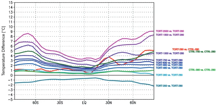
Zonal Average Temperatures

Figure 6 shows the zonal average tempera-tures of the simulations. The Miocene experiments are compared to the TORT-280 and the present-day runs, and TORT-280 y\to CTRL-280 respec-tively. TORT-280 were much warmer than CTRL-280 at in latitudes of 30°N (+4°C) and farther north (+5°C), whereas CTRL-280 and TORT-280 did not differ much (less than +1°C) at the equator. Thus, TORT-280 represents a weaker-than-present lati-tudinal temperature gradient of –4°C. The latitudi-nal gradient in TORT-200 was less pronounced than in TORT-280, but it was still weaker than in CTRL-280. With increasing carbon dioxide in the atmosphere, the all latitudes became successively warmer, but polar warming was much more intense. In TORT-INC at 2,000 ppm, the high lati-tudes heated up by +9°C compared to TORT-280, and tropical latitudes were +3.5°C warmer. Thus, FIGURE 3. The annual average of the present-day’s ocean flux correction [W/m2_{] used in all experiments.}

the temperature difference between pole and equator was 5.5°C lower than in TORT-280. The successive reduction of the latitudinal temperature gradient was a result of the sea ice-albedo feed-back (cf. Figures 4 and 5). The temperature differ-ence between TORT-2000 (i.e., TORT-INC at 2000 ppm) and TORT-1500 is generally less than for TORT-1500 vs. TORT-1000. The weaker response was due to the fact that northern sea ice vanisheed at around 1,400 ppm (Figure 5).

Between CTRL-360 and CTRL-280, there were only minor differences of less than +1°C, sim-ilar to the differences between TORT-360 and TORT-280. However, CTRL-700 vs. CTRL-280 as compared to CTRL-360 vs. CTRL-280 demon-strated greater polar warming than TORT-700 and TORT-360 vs. TORT-280, respectively. The CO2 doubling from 360 ppm to 700 ppm lead to a polar warming of +4°C under present-day conditions, whereas it is only +3°C in the Miocene. In lower lat-itudes, the response to the CO₂ increase was about the same. Thus, the sea ice-albedo feed-back tended to be weaker under Miocene bound-ary conditions than in present-day conditions (cf. Figure 4).

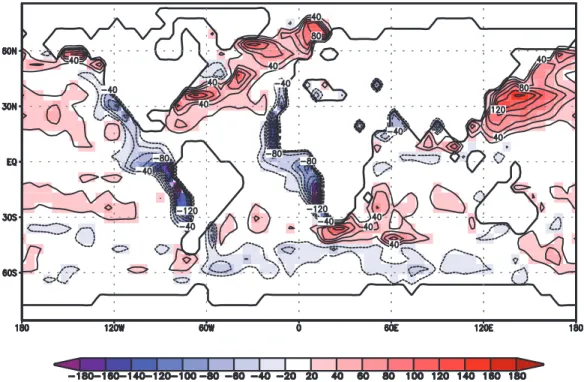
Spatial Temperature Anomalies

The spatial distributions of mean annual tem-perature and the sea ice margin in our simulations are shown in Figure 7. The increase of CO2 lead to a generally more pronounced warming in the pres-ent-day experiments as compared to the Miocene runs (Figure 7). For CTRL-280 to CTRL-700, the ice volume was greater than in TORT-200 to TORT-2000 (cf. sec. 3.1 and 3.2). Therefore, the ice-albedo feedback was more intense under pres-ent-day conditions. Moreover, the Paratethys dampened the effect of enhanced CO₂ in the Mio-cene simulations. In TORT-200 as compared to TORT-280, the cooling from decreased CO₂ occured primarily in higher latitudes. This pattern was a contrast to the other Tortonian runs. Gener-ally, the interior parts of the continents became warmer when CO2 increased. Not until a high con-centration of CO2 and ice-free conditions were reached, did polar warming reach the same order of magnitude as over continental areas. In Central Africa, temperatures in the Tortonian runs remained more or less the same with increasing CO₂; intensified evapotranspiration (evaporative cooling) dampened the temperature increase due to the greenhouse effect.

13.6 14.3 16.8 14.8 15.9 16.6 17.3 17.8 18.2 18.5 6.5 6.1 3.2 6.2 5.4 4.8 3.9 3.4 3.2 2.7 0 5 10 15 20 25 30 200 300 400 500 600 700 800 900 1000 1100 1200 1300 1400 1500 1600 1700 1800 1900 2000 2100 2200 p CO2 [ppm] Te m pe ra tur e [ °C ] 0 1 2 3 4 5 6 7 8 9 10 11 12 13 14 15 S ea I ce C over [% ]

FIGURE 4. The global averages of temperature [°C] (red, left axis) and sea ice cover [%] (blue, right axis) plotted against the atmospheric CO2 concentration [ppm]. The red and blue lines represent TORT-INC, diamonds illustrate

The Sensitivity Experiments vs. Quantitative Terrestrial Proxy Data

Steppuhn et al. (2007) established a method to compare Late Miocene model experiments with quantitative terrestrial proxy data. We used essen-tially the same method to test how consistent the mean annual temperatures (MAT) of the different Late Miocene CO₂ model runs compared to the fossil record. We used the terrestrial proxy data from Steppuhn et al. (2007). All data for mean annual temperature (MAT) are based on quantita-tive climate analyses of fossil plant remains from the Tortonian stage (early Late Miocene, ~ 11 to 7 Ma). For most of the data, the Coexistence Approach (Mosbrugger and Utescher 1997) was applied to micro- (pollen and spores) and macro-botanical (leaves, fruits, and seeds) fossils. The results of this method are ‘coexistence intervals,’ which express the minimum-maximum range of temperature at which a maximum number of taxa of a given flora can exist. Relying mainly on one

reconstruction method reduces the impact of meth-odological inconsistencies. However, such data are not available for North America so we also included some quantitative climate data based on the CLAMP technique (Wolfe 1993), which has proven to be a reliable method for climate quantification on the American continent (cf. Wolfe 1995, 1999).

Because such data usually do not include a minimum-maximum range of temperature, a stan-dard range of uncertainty of ±1 °C was assumed for the data-model-comparison. We augmented the Steppuhn et al. (2007) data set with additional cli-mate information from Wolfe et al. (1997) and new data from the NECLIME program (see http:// www.neclime.de) published by Akgün et al. (2007), Bruch et al. (2007) and Utescher et al. (2007). The actual data set used in this study now comprises 78 localities. Because most of the proxy data are minimum to maximum mean annual temperature per locality, Steppuhn et al. (2007) constructed a similar MAT range from the minimum and maxi-mum mean annual temperature range using

10-pCO

2

[ppm]

Sea Ice Cover [%]

FIGURE 5. The zonal average sea ice cover [%] of TORT-INC plotted against the CO2 concentration [ppm] (vertical

year-model integrations for those grid points that correspond to the palaeontologic localities. When both both climate intervals overlapped, model results and proxy data the temperature difference were considered to be zero; where the intervals did not overlap, the smallest distance between them was used as the measure of inconsistency between them. We modified the validation method of Steppuhn et al. (2007) because results of TORT-1000, TORT-1500, and TORT-2000 do not repre-sent a time series over 10 years. Instead of creat-ing temperature intervals from our simulations, we use point data. For TORT-1000 to TORT-2000, the point data are simply the mean annual tempera-tures of the years 900, 1400, and 1900, respec-tively. For TORT-200 to TORT-700, the point data were the mean annual temperatures averaged over the last 10 years of the model integrations. Except for this difference, our validation method followed the same principle as Steppuhn et al. (2007). Table 2 summarises the overall agreement of the Tortonian simulations with proxy data. In Fig-ure 8, the temperatFig-ure differences between the simulations and proxy data are mapped for all localities.

On the global scale (Table 2), the experiment TORT-280 fits the terrestrial proxy data best, but TORT-200, TORT-360, and TORT-460 are more or less consistent with them. Discrepancies of TORT-200 to TORT-460 are within ±1°C of the proxy data. These deviations from the fossil record are quite acceptable. As one might expect, TORT-2000

demonstrates the worst consistency with the proxy data and is globally much too warm.

Figure 8 shows details of the comparison of model results and proxy data. TORT-200 and TORT-280 globally demonstrate the best agree-ment to proxy data, but they are systematically too cool in higher latitudes. TORT-360 and TORT-460 indicate a better agreement in higher latitudes. However, both runs tended to be slightly too warm in the mid-latitudes, particularly in Europe. At the expense of heating up lower and mid-latitudes, TORT-560 to TORT-2000 were continuously more consistent with the high-latitude proxy data. Figure 8 illustrates that TORT-360 to TORT-560 agree best with the proxy data. This agreement seems to contradict Table 2, but one has to keep in mind that the proxy data are highly concentrated on Europe. Consequently, discrepancies in this region are over-weighted compared to others. Our results support a Late Miocene pCO2 in the range of 360 to 560 ppm.

DISCUSSION

We defined Late Miocene climate models 1) to test how much CO₂ is necessary to produce ice-free conditions on the Northern Hemisphere in the Miocene, 2) to analyse the Miocene climate sensi-tivity with respect to variations of CO₂, and 3) to validate the consistency of the model results with proxy data in order to estimate how high CO2 might have been in the Late Miocene.

TORT-280 vs. CTRL-280 TORT-360 vs. TORT-280 TORT-560 vs. TORT-280 TORT-460 vs. TORT-280 TORT-630 vs. TORT-280 TORT-700 vs. TORT-280 TORT-200 vs. TORT-280 TORT-1000 vs. TORT-280 TORT-1500 vs. TORT-280 TORT-2000 vs. TORT-280 CTRL-360 vs. CTRL-280 CTRL-700 vs. CTRL-280 Te mperature Dif ference [°C]

FIGURE 6. The zonal average temperature differences [°C]. TORT-280, CTRL-360, and CTRL-700 are shown as ifferences to CTRL-280, and TORT-200 to TORT-2000 are shown as differences to TORT-280, respectively.

How much CO2 is necessary to produce

ice-free conditions on the Northern Hemisphere in the Miocene? The first question can now be easily

answered: based on our model results, a pCO₂ of at least 1500 ppm is necessary to produce an ice-free Arctic Ocean. Even the most optimistic inde-pendent estimations of Miocene carbon dioxide concentrations give values of about 1000 ppm or

less (e.g., Cerling 1991; Retallack 2001). Thus, our model results suggest that other processes than CO2 are necessary to explain an ice-free Arctic Ocean in the Miocene. Recent evidence from the Miocene fossil record suggests some significant cooling events and supports the hypothesis that sea ice covered part of the Northern Hemisphere

CTRL-360 vs. CTRL-280 CTRL-700 vs. CTRL-280

TORT-280 vs. CTRL-280 TORT-200 vs. TORT-280

TORT-360 vs. TORT-280 TORT-460 vs. TORT-280

Annual Temperature Differences [°C]

FIGURE 7. The annual average temperature differences [°C] and sea ice margin (grey solid line). TORT-280, CTRL-360 and CTRL-700 are shown as differences to CTRL-280, and TORT-200 to TORT-2000 are shown as dif-ferences to TORT-280, respectively. Non-colored white areas in represent non-significant difdif-ferences with a Stu-dent’s t-test (p = 0.01) (continued on next page).

(e.g., Moran et al. 2006; Kamikuri et al. 2007; Jako-bsson et al. 2007).

What is the Late Miocene climate sensitivity with respect to different concentrations of CO2? Our present-day simulations, the global tempera-ture increased by 2.5°C between TORT-360 and TORT-700. McGuffie et al. (1999) demonstrated that a doubling of CO2 under present-day condi-tions leads to a warming of +2.5°C to +4.5°C. The most recent future climate change projections of the IPCC (Meehl et al. 2007), which consider a doubling of CO₂, give a similar temperature increase between +2°C to +4.5°C. Our present-day

sensitivity experiments are at the lower end of that prediction, but still within the range of these climate change scenarios. Our Late Miocene simulations demonstrate a global temperature increase of +1.9°C when atmospheric CO2 doubles (TORT-280 vs. TORT-560, TORT-360 vs. TORT-700). The Late Miocene climate sensitivity to changes in

pCO2 was weaker than today. Steppuhn et al. (2007) observed that a doubling of CO₂ under Mio-cene boundary conditions led to a global warming of +3°C. This is well within future climate change predictions, but stronger than we found in our sim-ulations. The sea ice cover in Steppuhn et al.’s

TORT-700 vs. TORT-280 TORT-1000 vs. TORT-280

TORT-1500 vs. TORT-280 TORT-2000 vs. TORT-280

TORT-560 vs. TORT-280 TORT-630 vs. TORT-280

Annual Temperature Differences [°C]

(2007) Tortonian reference run is close to the mod-ern situation. In our simulations, even TORT-200 had a lower ice volume than CTRL-360 (Figure 4). Thus, the lower sea ice-albedo feedback dampens the Late Miocene climate sensitivity to CO₂ increase, although the Late Miocene is still compa-rable to the modern situation. The amount of sea ice is lower in our Miocene simulations than in pre-vious Tortonian experiments (Micheels et al. 2007; Steppuhn et al. 2006, 2007) because we specified the modern ocean flux correction (Figure 3), whereas the previous studies considered a weaker-than-present ocean heat transport. The reduced sea ice cover in our Tortonian runs as compared to the present-day simulations is explained by the warming effect of Greenland (no glaciers and lower elevation, Figure 1) greater for-est cover (Figure 2). These results are consistent to the previous studies.

Future climate change projections also dem-onstrated that continents are more affected by global warming than are oceans (e.g., Meehl et al. 2007). This is consistent to our simulations. How-ever, other climate change predictions indicate a

pronounced warming of higher latitudes (e.g., Meehl et al. 2007), which is consistent with the changes between TORT-360 and TORT-700. In contrast, our Late Miocene simulations do not show as much high-latitude warming (Figure 4). The reduced ice-albedo feedback in the Tortonian runs as compared to the present-day situation reduces the high-latitude response to CO₂. In the lower latitudes, future climate change projections and our Miocene runs are quite comparable. In contrast to Steppuhn et al. (2007), the different boundary conditions between Miocene and mod-ern make a difference in the climate response to enhanced CO2-scenarios. In general, our Miocene experiments demonstrate a weaker sensitivity to higher CO2 than future climate change scenarios because sea ice is already reduced in the Miocene reference run.

How consistent are the different Late Miocene CO₂-scenarios as compared to the fossil record and can we estimate how high CO₂ was in the Late Miocene? Our model fits with proxy fossil data

quite well when pCO2 is between 360 to 560 ppm Table 2. The temperature differences [°C] between the Tortonian simulations and terrestrial proxy data averaged over all localities. EXP T [°C] T| [°C] TORT-200 -0.45 1.08 TORT-280 +0.42 1.09 TORT-360 +0.69 1.30 TORT-460 +1.07 1.48 TORT-560 +1.88 2.07 TORT-630 +1.94 2.12 TORT-700 +2.40 2.53 TORT-1000 +3.53 3.61 TORT-1500 +4.99 5.03 TORT-2000 +6.50 6.50

(Figure 8). TORT-200 to TORT-460 produced a global temperature that was less than ±1°C differ-ent from the proxy data. Micheels et al. (2007) found a global discrepancy to proxy data of –2.4°C in a Tortonian simulation with the AGCM ECHAM4/ ML using almost the same boundary conditions and proxy data base. If discrepancy of this

magni-tude is acceptable, then even TORT-700 is a real-istic scenario for the Late Miocene (Table 2).

There are, however, some crucial points which limit our interpretations. Most Late Miocene fossil proxy data cover the European realm, whereas most other key regions such as the high latitudes, Africa and Asia are poorly covered. Our

TORT-200 TORT-280

TORT-360 TORT-460

TORT-560 TORT-630

Model vs. Proxy Data Temperature Differences [°C]

FIGURE 8. The mean annual temperature differences [°C] between TORT-200 to TORT-2000 and terrestrial proxy data (continued on next page).

sensitivity runs demonstrate that lower to mid-lati-tudes are warmer than suggested by proxy data, but this statement is based on only a few localities. With regard to the quality of proxy data, there are some shortcomings that may influence detailed data comparisons. This includes the time span cov-ered by the proxy data, which may hide temporal climatic variability, palaeogeographical changes, which may change the exact position of data points with respect to the grid cell (e.g. in the Pannonian realm, cf. Erdei et al. 2007), and possible tapho-nomic biases, which may influence the results of different reconstruction methods (e.g., Liang et al. 2003; Uhl et al. 2003, 2006). Despite some possi-ble shortcomings, quantitative climate proxy data based on plant fossils are consistent on a larger scale (Bruch et al. 2004, 2006, 2007), and they

provide reliable information to validate global cli-mate model results (Micheels et al. 2007; Step-puhn et al. 2007).

For our purposes, we consider the proxy data to be more reliable than our model results. The model experiments can be unrealistic because of weak points in the model and its boundary condi-tions. The EMIC Planet Simulator with its simplified parameterisation schemes and the boundary con-ditions explain rather more inconsistencies in our experiments. For some localities (e.g., in Africa, North America), the orography in the model might be unrealistic because of the coarse model resolu-tion, the spectral transformation method or simply because the reconstruction of the orography is not fully correct. The coarse model resolution also does not allow for representation of details of the

TORT-700 TORT-1000

TORT-1500 TORT-2000

Model vs. Proxy Data Temperature Differences [°C]

< -10 -10 to -5 -4 to -5 -3 to -4 -2 to -3 -1 to -2 ±1 > +10 +10 to +5 +4 to +5 +3 to +4 +2 to +3 +1 to +2

land-sea distribution. For example, the model can-not resolve Iceland (Figure 8), which may explain why the changes between 200 and TORT-630 indicate conditions in the North Atlantic region that are too cool. In addition, our settings for the ocean include some uncertainties. As mentioned in the model description, the sea ice model tends to overestimate the amount of ice and the perfor-mance of the ice model for annual ice is better than for perennial ice. However, with increasing CO₂ concentrations in our runs, the amount of perennial ice decreases, and the model performance should improve. The absence of ocean and sea-ice dynamics is a potential source of errors in our study, but it is computationally expensive to run fully-coupled atmosphere-ocean general circula-tion models in particular for a series of sensitivity experiments.

For this reason, AGCM experiments for the Miocene used either prescribed sea surface tem-peratures and sea ice (e.g., Ramstein et al. 1997; Lunt et al. 2008) or slab ocean models (e.g., Dut-ton and Barron 1997; Micheels et al. 2007). For past climates, ocean dynamics plays an important role (e.g., Bice et al. 2000). Due to an open Pan-ama Isthmus, the northward heat transport in the Atlantic Ocean was weaker than today in the Mio-cene (e.g., Bice et al. 2000; Steppuhn et al. 2006). Because of using the present-day flux correction, the climate in Europe should be too warm in our sensitivity experiments. If we consider that temper-atures in Europe might need to be corrected to slightly cooler conditions, the scenarios TORT-460 to TORT-630 would be more realistic. Taking all weak points into account, the scenarios TORT-360 and TORT460 fit best with the fossil record. Hence with some limitations, the simulations support a slightly higher-than-present (intermediate) pCO2 between 360 ppm and 460 ppm in the Late Mio-cene. Consistent with this result, MacFadden (2005) proposed a pCO2 of 500 ppm in the Mio-cene, and Haywood and Valdes (2004, 2006) pro-posed a pCO2 of 400 ppm for the Middle Pliocene.

SUMMARY AND CONCLUSIONS

We performed CO₂-sensitivity experiments for the Late Miocene using the earth system model of intermediate complexity Planet Simulator. We modelled CO2 concentrations ranging from 200 to 2000 ppm, with all other boundary conditions unchanged. We found that:

•

An atmospheric carbon dioxide of 1500 ppm is necessary to produce an ice-free Northern Hemisphere in our model. This value is much too high to be reasonable for the Miocene (e.g., Cerling 1991; Retallack 2001). Our sen-sitivity experiments support evidences for an onset of the Northern Hemisphere’s glaciation before the Miocene (e.g., Moran et al. 2006; Kamikuri et al. 2007; Jakobsson et al. 2007).

•

The climate sensitivity to enhanced

concen-trations of greenhouse gases is reduced in the Late Miocene compared to the modern world. The Late Miocene represents a hothouse cli-mate with a reduced ice cover, which damp-ens the ice-albedo feedback. However, the climate response to increases in CO₂ is only slightly weaker than in future climate change scenarios (e.g., Meehl et al. 2007). With some limitations, the Late Miocene can serve as an analogue for the future situation.

•

The Late Miocene simulations with a pCO2 from 280 to 630 ppm agree reasonably well with quantitative terrestrial fossil proxy data. At higher CO2 levels, the consistency with proxy data becomes progressively worse. Based on our results, an intermediate concentration of CO₂ between 360 and 460 ppm is realistic for the Late Miocene.

The results of our modelling experiment should not be over-interpreted because of uncer-tainties in the model (e.g., simplified physical parameterisations) and certain features of the model configuration (e.g., the ocean setup). The agreement between our model results and proxy data emphasises the need for proxy data from cru-cial regions such as the high latitudes and Africa. More quantitative climate information from the fos-sil record from these poorly covered regions would be helpful to better estimate the reliability of climate model experiments.

ACKNOWLEDGEMENTS

We gratefully acknowledge the comments of our two anonymous reviewers, which helped to improve our manuscript. The authors would like to thank the Deutsche Forschungsgemeinschaft within the project “Understanding Cenozoic Cli-mate Cooling” (FOR 1070) and the federal state Hessen (Germany) within the LOEWE initiative for their financial support. This work is a contribution to the program “Neogene Climate Evolution in Eur-asia – NECLIME.”

REFERENCES

Akgün, F., Kayseri, M.S., and Akkiraz, M.S. 2007. Palae-oclimatic evolution and vegetational changes during the Late Oligocene – Miocene period in Western and Central Anatolia (Turkey). Palaeogeography, Palaeo-climatology, Palaeoecology, 253, 56-90.

Bartoli, G., Sarnthein, M., Weinelt, M., Erlenkeuser, H., Garbe-Schönberg, D., and Lea, D.W. 2005. Final clo-sure of Panama and the onset of northern hemi-sphere glaciation. Earth and Planetary Science Letters, 237, 33-44.

Bice, K.L., Scotese, C.R., Seidov, D., Barron, and E.J. 2000. Quantifying the role of geographic change in Cenozoic ocean heat transport using uncoupled atmosphere and ocean models, Palaeogeography Palaeoclimatology Palaeoecology, 161, 295-310. Bruch, A.A., Utescher, T., Alcalde Olivares, C.,

Dolak-ova, N., and Mosbrugger, V. 2004. Middle and Late Miocene spatial temperature patterns and gradients in Central Europe – preliminary results based on paleobotanical climate reconstructions. Courier Forschungsinstitut Senckenberg, 249, 15-27. Bruch, A.A., Utescher, T., Mosbrugger, V., Gabrielyan, I.,

and Ivanov, D.A. 2006. Late Miocene climate in the circum-Alpine realm-a quantitative analysis of terres-trial paleofloras. Palaeogeography Palaeoclimatol-ogy PalaeoecolPalaeoclimatol-ogy, 238, 270-280.

Bruch, A.A., Uhl, D., and Mosbrugger, V. 2007. Miocene climate in Europe – Patterns and evolution: A first synthesis of NECLIME. Palaeogeography Palaeocli-matology Palaeoecology, 253, 1-7.

Cerling, T.E. 1991. Carbon dioxide in the atmosphere: evidence from Cenozoic and Mesozoic paleosols. American Journal of Science, 291, 377-400.

Collins, L., Coates, A.G., Berggren, W.A., Aubry, M.-P., and Zhang, J. 1996. The late Miocene Panama isth-mian strait. Geology, 24, 687-690.

Cubasch, U., Meehl, G.A., Boer, G.J., Stouffer, R.J., Dix, M., Noda, A., Senior, C.A., Raper, S., and Yap, K.S. 2001. Projections of Future Climate Change. In Houghton, J.T., Y. Ding, D.J. Griggs, M. Noguer, P.J. van der Linden, X. Dai, K. Maskell, C.A. Johnson (eds.), Climate Change 2001: The Scientific Basis. Contribution of Working Group I to the Third Assess-ment Report of the IntergovernAssess-mental Panel on Cli-mate Change. Cambridge University Press, Cambridge, 525-582.

Dutton, J.F., and Barron, E.J. 1997. Miocene to present vegetation changes: A possible piece of the Ceno-zoic puzzle. Geology, 25(1), 39-41.

Erdei, B., Hably, L., Kázmér, M., Utescher. T., and Bruch, A.A. 2007. Neogene flora and vegetation develop-ment in the Pannonian Basin - relations to palaeocli-mate and palaeogeography. Palaeogeography Palaeoclimatology Palaeoecology, 253, 115-140.

Fraedrich, K., Kirk, E.,, and Lunkeit, F. 1998. PUMA: Por-table University Model of the atmosphere. DKRZ Technical Report, 16, Max-Planck-Institut für Meteo-rologie, 24 pp, http://www.mad.zmaw.de/fileadmin/ extern/documents/reports/ReportNo.16.pdf.

Fraedrich, K., Jansen, H., Kirk, E., Luksch, U., and Lunkeit, F. 2005a. The Planet Simulator: Towards a user friendly model. Meteorologische Zeitschrift, 14, 299-304, http://www.mi.uni-hamburg.de/fileadmin/ files/forschung/theomet/planet_simulator/downloads/ plasim_mz_1.pdf.

Fraedrich, K., Jansen, H., Kirk, E., and Lunkeit, F. 2005b. The Planet Simulator: Green planet and desert world. Meteorologische Zeitschrift, 14, 305-314, http:// www.mi.uni-hamburg.de/fileadmin/files/forschung/ theomet/planet_simulator/downloads/

plasim_mz_2.pdf.

Haywood, A.M., Sellwood, B.W., and Valdes, P.J. 2000a. Regional warming: Pliocene (ca. 3 Ma) Paleoclimate of Europe and the Mediterranean. Geology, 28, 1063-1066.

Haywood, A.M., Valdes, P.J., and Sellwood, B.W. 2000b. Global scale paleoclimate reconstruction of the mid-dle Pliocene Climate using the UKMO GCM: initial results. Global and Planetary Change, 25, 239-256. Haywood, A.M., and Valdes, P.J. 2004. Modelling

Plio-cene warmth: contribution of atmosphere, oceans and cryosphere. Earth and Planetary Science Let-ters, 218, 363-377.

Haywood, A.M., and Valdes, P.J. 2006. Vegetation cover in a warmer world simulated using a dynamic global vegetation model for the Mid-Pliocene. Palaeogeog-raphy, Palaeoclimatology, Palaeoecology, 237, 412-427.

Helland, P.E., and Holmes, M.A. 1997. Surface textural analysis of quartz sand grains from ODP Site 918 off the southeast coast of Greenland suggests glaciation of southern Greenland at 11Ma. Palaeogeography Palaeoclimatology Palaeoecology, 135, 109-121. Jakobsson, M., Backman, J., Rudels, B., Nycander, J.,

Frank, M., Mayer, L., Jokat, W., Sangiorgi, F., O’Regan, M., Brinkhuis, H., King, J., and Moran, K. 2007. The early Miocene onset of a ventilated circu-lation regime in the Arctic Ocean. Nature, 447, 986-990.

Junge, M.M., Lunkeit, F., Fraedrich, K., Gayler, V., Blender, R., and Luksch, U. 2004. A world without Greenland: impacts on northern hemisphere circula-tion in low and high resolucircula-tion models. Climate Dynamics, 24, 297-307.

Kamikuri, S., Nishi, H., and Motoyama, I. 2007. Effects of late Neogene climatic cooling on North Pacific radio-larian assemblages and oceanographic conditions. Palaeogeography Palaeoclimatology Palaeoecol-ogy, 249, 370-392.

Kleiven, H.F., Jansen, E., Fronval, T., and Smith, T.M. 2002. Intensification of Northern Hemisphere glacia-tions in the circum Atlantic region (3.5 – 2.4 Ma) – ice-rafted detritus evidence. Palaeogeography Palaeoclimatology Palaeoecology, 184, 213-223. Kutzbach, J.E., and Behling, P. 2004. Comparison of

simulated changes of climate in Asia for two scenar-ios: Early Miocene to present, and present to future enhanced greenhouse. Global and Planetary Change, 41, 157-165.

Liang, M.,Bruch, A.A., Collinson, M., Mosbrugger, V., Li, C., Sun, Q., and Hilton, J. 2003. Testing the climatic signals from different palaeobotanical methods: an example from the Middle Miocene Shanwang flora of China. Palaeogeography, Palaeoclimatology, Palae-oecology, 198, 279-301.

Lunkeit, F., Böttinger, M., Fraedrich, K., Jansen, H., Kirk, E., Kleidon, A., and Luksch, U. 2007. Planet Simula-tor Reference Manual Version 15.0. http:// www.mi.uni-hamburg.de/fileadmin/files/forschung/ theomet/planet_simulator/downloads/

PS_ReferenceGuide.pdf.

Lunt, D.J., Flecker, R., Valdes, P.J., Salzmann, U., Glad-stone, R., and Haywood, A.M. 2008. A methodology for targeting palaeo proxy data acquisition: A case study for the terrestrial late Miocene. Earth and Plan-etary Science Letters, 271, 53-62.

MacFadden, B.J. 2005. Terrestrial Mammalian Herbivore Response to Declining Levels of Atmospheric CO₂ During the Cenozoic: Evidence from North American Fossil Horses (Family Equidae). In Ehleringer, J.R, Cerling, T.E., and Dearing, M.D. (eds.). A History of Atmospheric CO2 and Its Effects on Plants, Animals,

and Ecosystems. Ecological Studies, 177, 273-292. McGuffie, K., Henderson-Sellers, A., Holbrook, N.,

Kothavala, Z., Balcjova, O., and Hoekstra, J. 1999. Assessing simulations of daily temperatures and pre-cipitation variability with global climate models for present and enhanced greenhouse climates. Interna-tional Journal of Climatology, 19, 1-26.

Meehl, G.A., Stocker, T.F., Collins, W.D., Friedlingstein, P., Gaye, A.T., Gregory, J.M., Kitoh, A., Knutti, R., Murphy, J.M., Noda, A., Raper, S.C.B., Watterson, I.G., Weaver, A.J., and Zhao, Z.-C., 2007. Regional Climate Projections. In Solomon, S., Qin, D., Man-ning, M., Chen, Z., Marquis, M., Averyt, K.B., Tignor, M., and Miller H.L. (eds.). Climate Change 2007: The Physical Science Basis. Contribution of Working Group I to the Fourth Assessment Report of the Inter-governmental Panel on Climate Change. Cambridge University Press, Cambridge, United Kingdom and New York, NY, USA, 747-845.

Micheels, A., Bruch, A.A., Uhl, D., Utescher, T., and Mos-brugger, V. 2007. A Late Miocene climate model sim-ulation with ECHAM4/ML and its quantitative validation with terrestrial proxy data.

Palaeogeogra-phy, Palaeoclimatology, Palaeoecology, 253,

267-286.

Micheels, A., Eronen, J., and Mosbrugger, V. (2009). The Late Miocene climate response on a modern Sahara desert. Global and Planetary Change, 67, 193-204. Molnar, P. 2005. Mio-Pliocene Growth of the Tibetan

Pla-teau and Evolution of East Asian Climate.

Paleonto-logia Electronica, 8(1), 1-23,

http://paleo-electronica.org/paleo/2005_1/molnar2/ issue1_05.htm.

Moran, K., Backman, J., Brinkhuis, H., Clemens, S.C., Cronin, T., Dickens, G.R., Eynaud, F. , Gattacceca, J., Jakobsson, M., Jordan, R.W., Kaminski, M., King, J., Koc, N., Krylov, A., Martinez, N., Matthiessen, J., McInroy, D., Moore, T.C., Onodera, J., O’Regan, M., Pälike, H., Rea, B., Rio, D., Sakamoto, T., Smith, D.C., Stein, R., St John, K., Suto, I., Suzuki, N., Taka-hashi, K., Watanabe, M., Yamamoto, M., Farrell, J., Frank, M., Kubik, P., Jokat, W., Kristoffersen, Y., 2006. The Cenozoic palaeoenvironment of the Arctic Ocean. Nature, 441, 601-605.

Mosbrugger, V., and Utescher, T. 1997. The coexistence approach - a method for quantitative reconstructions of Tertiary terrestrial palaeoclimate data using plant fossils. Palaeogeography, Palaeoclimatology, Palae-oecology, 134, 61-86.

Mosbrugger, V., Utescher, T., and Dilcher, D.L. 2005. Cenozoic continental climatic evolution of Central Europe. Proceedings of the National Academy of Sci-ence, 102, 14964-14969.

Pagani, M., Zachos, J.C., Freeman, K.H., Tipple, B., and Bohaty, S. 2005. Marked decline in atmospheric car-bon dioxide concentrations during the Paleogene. Science, 309, 600-603.

Pearson, P.N., and Palmer, M.R. 2000. Atmospheric car-bon dioxide concentrations over the past 60 million years. Nature, 406, 695-699.

Petit, J.R., Jouzel, J., Raynaud, D., Barkov, N.I., Barnola, J.M., Basile, I., Bender, M., Chappellaz, J., Davis, J., Delaygue, G., Delmotte, M., Kotlyakov, V.M., Legrand, M., Lipenkov, V., Lorius, C., Pépin, L., Ritz, C., Saltzman, E., and Stievenard M. 1999. Climate and Atmospheric History of the Past 420,000 years from the Vostok Ice Core, Antarctica. Nature, 399, 429-436.

Popov, S.V., Rögl, F., Rozanov, A.Y., Steininger, F.F., Shcherba, I.G., and Kovac, M. 2004. Lithological-paleogeographic maps of Paratethys. 10 maps Late Eocene to Pliocene. Courier Forschungsinstitut Senckenberg, 250, 1-46.

Ramstein, G., Fluteau, F., Besse, J., and Joussaume, S. 1997. Effect of orogeny, plate motion and land-sea distribution on Eurasian climate change over past 30 million years. Nature, 386, 788-795.

Retallack, G. 2001. Cenozoic expansion of grasslands and climatic cooling. Journal of Geology, 109, 407-426.

Roeckner, E., Bäuml, G., Bonaventura, L., Brokopf, R., Esch, M., Giorgetta, M., Hagemann, S., Kirchner, I., Kornblueh, L., Manzini, E., Rhodin, A., Schlese, U., Schulzweida, U., and Tompkins, A. 2003. The atmo-spheric general circulation model ECHAM5 Part I – Model description. Max Planck Institute for Meteorol-ogy, Report No. 349, 127 pp.

Roeckner, E., Brokopf, R., Esch, M., Giorgetta, M., Hagemann, S., Kornblueh, L., Manzini, E., Schlese, U., and Schulzweida, U. 2006. Sensitivity of simu-lated climate to horizontal and vertical resolution in the ECHAM5 atmosphere model. Journal of Climate, 19, 3771-3791.

Ruddiman, W.F., Kutzbach, J.E., and Prentice, I.C. 1997. Testing the climatic effects of orography and CO₂ with general circulation and biome models. In Ruddi-man,W.F. (ed.), Tectonic Uplift and Climate Change. Plenum, New York, 203-235.

Semtner, A.J. Jr. 1976. A Model for the Thermodynamic Growth of Sea Ice in Numerical Investigations of Cli-mate, Journal of Physical Oceanography, 3, 379-389. Spicer, R.A., Harris, N.B.W., Widdowson, M., Herman, A.B., Guo, S., Valdes, P.J., Wolfe, J.A., and Kelley, S.P. 2003. Constant elevation of southern Tibet over the past 15 million years. Nature, 421, 622-624. St. John, K.E.K., and Krissek, L.A. 2002. The late

Mio-cene to PleistoMio-cene ice-rafting history of southeast Greenland. Boreas, 31, 28-35.

Steppuhn, A., Micheels, A., Geiger, G., and Mosbrugger, V. 2006. Reconstructing the Late Miocene climate and oceanic heat flux using the AGCM ECHAM4 coupled to a mixed-layer ocean model with adjusted flux correction, Palaeogeography, Palaeoclimatology, Palaeoecology, 238, 399-423.

Steppuhn, A., Micheels, A., Bruch, A.A., Uhl, D., Ute-scher, T., and Mosbrugger, V. 2007. The sensitivity of ECHAM4/ML to a double CO2 scenario for the Late

Miocene and the comparison to terrestrial proxy data. Global and Planetary Change, 57, 189-212.

Tong, J.A., You, Y., Müller, R.D., and Seton, M. 2009. Cli-mate model sensitivity to atmospheric CO₂ concen-trations for the Middle Miocene. Global and Planetary Change. doi: 10.1016/j.gloplacha.2009.02.001

Uhl, D., Mosbrugger, V., Bruch, A.A., and Utescher, T. 2003. Reconstructing palaeotemperatures using leaf floras – case studies for a comparison of leaf margin analysis and the coexistence approach. Review of Palaeobotany and Palynology, 126, 49-64.

Uhl, D., Bruch, A.A., Traiser, Ch., and Klotz, S. 2006. Palaeoclimate estimates for the Middle Miocene Schrotzburg flora (S-Germany) – A multi-method approach. International Journal of Earth Sciences, 95, 1071–1085.

Utescher, T., Djordjevic-Milutinovic, D., Bruch, A., and Mosbrugger, V. 2007. Palaeoclimate and vegetation change in Serbia during the last 30 Ma, Palaeogeog-raphy, Palaeoclimatology, Palaeoecology, 253, 141-152.

Winkler, A., Wolf-Welling, T.C.W., Stattegger, K., and Thiede, J. 2002. Clay mineral sedimentation in high northern latitude deep-sea basins since the Middle Miocene (ODP Leg 151, NAAG). International Jour-nal of Earth Sciences (Geologische Rundschau), 91, 133-148, DOI 10.1007/s005310100199.

Wolfe, J.A. 1993. A method of obtaining climatic parame-ters from leaf assemblages. U.S. Geological Survey Bulletin, 2040, 73 pp.

Wolfe, J.A. 1994a. Tertiary climatic changes at middle latitudes of western North America. Palaeogeogra-phy, Palaeoclimatology, Palaeoecology, 108, 195-205.

Wolfe, J.A. 1994b. An analysis of Neogene climates in Beringia. Palaeogeography, Palaeoclimatology, Palaeoecology, 108, 207-216.

Wolfe, J.A. 1995. Paleoclimatic estimates from Tertiary leaf assemblages. Annual Reviews of Earth and Planetary Sciences, 23, 119-142.

Wolfe, J.A. 1999. Early Palaeocene palaeoclimatic inferences from fossil floras of the western interior, USA -comment. Palaeogeography, Palaeoclimatology, Palaeoecology 150, 343-345.

Wolfe, J.A., Schorn, H.E., Forest, C.E., and Molnar, P. 1997. Paleobotanical evidence for high altitudes in Nevada during the Miocene. Science, 276, 1672-1675.

Zachos, J., Pagani, M., Sloan, L., Thomas, E., and Bil-lups, K. 2001. Trends, rhythms, and aberrations in global climate 65 Ma to present. Science, 292, 686-693.