DHISC : Disk Health Indexing System for Centers of Data Management

DHISC: Disk Health Indexing System for Centers of Data Management

by Rebecca Kekelishvili

Submitted to the

Department of Electrical Engineering and Computer Science In Partial Fulfillment of

the Requirements for the Degree of

Master of Engineering in Electrical Engineering and Computer Science

at the

Massachusetts Institute of Technology

June, 2017

M A SUCH USETS1 NST ITUT E OF T gHNQLOGY

LIBRARIES

ARCHIVES

(

2017 Massachusetts Institute of Technology. All rights reserved.

Signature redacted

May 26, 2017

Certified by:

Signature redacted

Ktrina LatuJrts, Lecturer for MIT EECS, Thesis Supervisor May 26, 2017

Certified by

Signature redacted

Wayne Booth, Director of Storage Engineering at NetApp, Thesis Co-Supervisor May 26, 2017

Accepted by:_

Signature redacted

Christopher JiTiiA, Chairman, Masters of Engineering Thesis Committee

Author:

DHISC: Disk Health Indexing System for Centers of Data Managements

by Rebecca Kekelishvili

Submitted to the

Department of Electrical Engineering and Computer Science In Partial Fulfillment of the Requirements for the Degree of

Master of Engineering in Electrical Engineering and Computer Science at the

Massachusetts Institute of Technology June, 2017

0 2017 Massachusetts Institute of Technology. All rights reserved.

Abstract

If we want to have reliable data centers, we must improve reliability at the lowest level of data storage -at the disk level. To improve reliability, we need to convert storage systems from reactive mechanisms that handle disk failures to a proactive mechanism that predict and address failures. Because the definition of disk failure is specific to a customer rather than defined by a standard, we developed a relative disk health metric and proposed a customer-oriented disk-maintenance pipeline. We designed a program that processes data collected from data center disks into a format that is easy to analyze using machine learning. Then, we used a neural network to recognize disks that show signs of oncoming failure with 95.4-98.7% accuracy, and used the result of the network to produce a rank of most and least reliable disks at the data center, enabling customers to perform bulk disk maintenance, decreasing system downtime.

Chapter 1. M otivation ... 4

1.1 Today's Disk Failure Pipeline ... 4

1.2 Definition of Disk Failure in Industry ... 8

1.3 Problem with Today's Disk Failure Pipeline ... 11

1 .4 O u r G o als ... 1 5 Chapter 2. DHISC Philosophy ... 17

2 .1 C h a lle n g e s ... 1 7 2 .2 P rio r W o rk ... 1 8 2.3 Our Approach ... 21

2.4 Contributions ... 22

Chapter 3. DHISC Design ... 25

3 .1 O v e rv ie w ... _{2 5} 2.2 DHISC Architecture ... ₂₇

2.3 The DHI Computer's Layering M odel ... 30

Chapter 4. Predicting Disk Failure ... 36

4.1 Overview ... ₃₆

4.2 Neural Network Basics ... ₃₉

4.3 Neural Network Design ... 45

4.4 Training Data ... ₄₈

4.5 Computing the DHI ... ₅₇

Chapter S. Evaluation ... ₅₈

5.1 DHI Performance ... ₅₈

5.2 Neural Network Configurations ... 65

5.3 Performance in Space ... 70

5.4 Performance in Speed ... 71

5.5 Alternative to Neural Networks ... ₇₂

Chapter 6. Discussion ... ₇₅

6.1 DHI and Failure M odes ... ₇₅

6 .2 .S ca la b ility ... 8 0 6 .3 A p p lica b ility ... 8 1 C o n clu sio n ... _{8 3} W orks Cited ... ₈₅

1.1 TODAY'S DISK FAILURE PIPELINE

In 2007, 90% of emerging electronically stored data was stored on magnetic media [1].

Despite the introduction of SSDs into the market, Google started experimenting with new designs

for HDDs as recently as 2016 [2], building them taller and taking advantage of the fact that disks

usually work in clusters. Disks are incredibly efficient for continuous data storage such as video,

and video streaming is estimated to become 80% of customer internet traffic by 2019. [3] Hard

Disk Drives are the most used of magnetic media, and despite their popularity and the necessity

for high performing disks in big data centers, there is no universal way to measure disk

performance or predict oncoming failure, as evidenced by the fact that companies such as

NETAPP, holding 7.9% market share in enterprise storage systems [4], do not use predictive analytics. [26] This thesis was done in collaboration with NETAPP, so henceforth, we use NETAPP

as the model for how disks are.managed in the corporate setting. I will give an example of how

NetApp manages hard disks in their data centers, and how this management can be improved

using predictive analytics, which I will also contribute. While other companies might have a

different pipeline for disk management, they can apply the techniques discussed in this thesis to

their business. (See 1.1.1.)

At NETAPP, disks operate within the scope of Data ONTAP, which is a customer operating

system that NETAPP designed for its storage solutions. Data ONTAP is a software manager which

sits on top of physical assets in the storage system. Before we continue, I will present a simplified

version of storage architecture to set up the landscape for how predictive analytics can fit into the

At the lowest level of the storage system, we have the physical Disk Layer. This is where

physical disks sit and are used as basic units of data storage. These disks can be either of consumer

or enterprise grade. At NetApp, there are four labels to indicate disk status: Data, Spare,

Pre-Failed, Pre-Failed, and Broken. A Data Disk reads and writes data when clients issue 1/O requests. A

Spare is an idle disk, kept in the system in case one of the Data Disks fails. A Pre-Failed Disk is one that encountered enough errors to cause worry, but has not yet been tested for failure. A Failed

Disk is one that RAID Layer (see below) [6] rendered unusable; Failed Disks need to be replaced. [8] A Broken Disk is one that was failed by the RAID Layer and consequently determined as unusable via a series of tests conducted engineers at a

-Lyseparate

Maintenance

task within an allotted time This layer also collects data on

y y disk performance - how many I/Os were read/written,

how many mistakes were made. An example of such a

sCS________yer__ mistake is a read/write that timed out, meaning that a disk

was unresponsive during a set period. Another example is

a Medium Error, a mismatch between data sent by the user

Figue1:Simplified storagearchitectureatlower _{and the data that was recorded, often detected via a}

checksum [25]. On top of the disk layer, there is a SCSI protocol layer, which lets disks

communicate with the rest of the storage system.

A software layer called System Health Monitor (SHM) sits on top of the Disk Layer. SHM counts errors propagated up from the Disk Layer within multiple time frames (10 minutes, a day,

a week). If a disk produces more errors than SHM allows, SHM sends the information about the

misbehaving disk to the Maintenance Center and RAID. RAID and Maintenance Center can be

thought of as a single layer, where Maintenance Center is a module that tests the disks, while RAID

has the executive control over reconstruction, copying data, and failing disks.

When the SHM passes information about a disk to this group, RAID automatically considers

the disk Pre-Failed and copies the contents of the suspected disk to another disk in the storage

system. [9] If a copy is unsuccessful, RAID performs reconstruction - a slow process that uses data

from disks that were in the same data volume as the misbehaving disk to extrapolate the kind of

data that the misbehaving disk held so that it can put it on a new Spare Disk. [6]

Then, Maintenance Center Software subjects the misbehaving disk to several tests

consisting of quick read/write loads intended to see if there is a fundamental problem with the

disk, or if the anomaly reported by SHM wasjust that - an anomaly. [7] The job of the Maintenance

Center is to determine the status of the disk. If the Maintenance Center Software checks several

sectors on the disk and finds that disk was capable of producing the data on those sections in

response to I/Os, then the disk is labeled as a Spare and returned to the general pool of disks inside

the storage system, along with Data disks. The disks that do not pass these tests are recommended

for failure to RAID. Out of the disks that are propagated to the Maintenance Center Software for

testing, 50% get returned as a Spare and the other 50% is recommended for failure [Figure 2] [6].

Afterwards, RAID receives the Maintenance Center Recommendation for failure, in a form

of a system message, and issues a command to offline the disk. At this point, the disk's status

When a disk is labeled as Failed, it is removed from the storage system manually. They are

then physically shipped to what is known as 3PR (3 rd Party Repair) site. At the test site, the disks

are subjected to a scrub and more thorough testing. Instead of running just a few tests on several

sectors like the Maintenance Center did, 3PR are more through and test the entire disk and run

much bigger loads. While a Maintenance Center test might take just 15 minutes, 3PR testing can

take a day or more, depending on the size of a disk.

Spare

spare

Shipped via UPS

- Shipped via UPS Spares' Depot

Shipped via UPS

3PR Test Site

Shipped via UPS

Vendor

Figure 2: NetApp systems consist of a computer called a Filer, displayed in black in the upper part of the image. This is where ONTAP, NetApp's operating system is running. ONTAP manages disks and storage layers above it. This figure is concerned only with the lifetime of disks within the system, where system is defined as filer, physical disks and software running on top of them. When a disk encounters more than a certain number of errors, it is labeled as pre-failed and then software called "Maintenance Center" runs i/o tests on several sectors of the disk. If a disk passes, it is returned into the general pool of disks in the system. Otherwise, it is labeled as failed and physically shipped to a separate facility called the Test Site, where it is separately tested. If the disk passes tests at the Test Site, it is then shipped to a facility that

holds spare disks for NetApp's use. Otherwise, the test is labeled as broken an d shipped to a vendor and it stops being the property of NetApp.

separate facility called the Spares' Depot. This is where Spare Disks are held before they become

in demand by a storage system somewhere at a NetApp site.

The reason that the longer 3PR tests are not conducted within ONTAP is because NetApp

is a data management company - they provide data systems to their clients. The systems include

the Filer (computer) that runs Data ONTAP and the disk shelves where the data is stored. Clients

want their storage solutions to be as simple as possible, so NetApp outsources these more

complicated tests to an outside facility, instead of having the lengthy checks done at customers'

sites. This is a decision driven by consideration for the customer, rather than technological

capabilities.

1.2 DEFINITION OF DISK FAILURE IN INDUSTRY

There is no single definition of disk failure in the storage industry, because there are too

many. definitions. To know how we can predict failures, we first must understand the different

players in the storage industry and how they define failures and why. In our simplified model of

the storage world, there are three main actors: Disk Manufacturers (those who produce and sell

disks, Storage Providers (such as NetApp), and Customers (those who buy storage systems that use

disks to store customer data).

To identify disk failure, Disk Manufacturers use SMART - Self Monitoring Analysis and

Reporting Technology [25, 26, 27]. SMART is a collection of over 240 metrics (such as temperature,

hours the disks was used, etc.) that Disk Manufacturers collect and sell for profit to storage

providers who buy disks from them. SMART is also used by the man ufacturer to debug a nd identify

and to have as few disks fail during the warranty period as possible (because this yields a greater

profit).

From the perspective of the Disk Manufacturer, a disk fails when it cannot pass the

manufacturer's test suite, consisting of workloads that they keep private [26]. From the

perspective of Storage Provides such as NetApp, a disk fails when it starts to fail their Customers

by causing latency spikes or frequent errors. The Customer does not want to manage disks on an individual level, which is why they hire NetApp to manage their data [26]. These perspectives lead

to a discrepancy between the percentage of disks reported as failed by the manufacturer and the

percentage of disks reported as failed by Storage Providers and other consumers of drives.

A study done by Google cited that "drive manufacturers often quote yearly failure rates below 2%" [1, 10] while industry numbers quoted by customers of drive manufacturers - Storage

Providers and individual buyers - are as high as 6% [1, 11]. Google also cited that "between

15-60% of drives considered to have failed at the user site are found to have no defect by the manufacturers upon returning the unit" [1, 13]. This finding can be explained by assuming that

manufacturers have a rigid definition of failure to minimize number of disks they have to repair at

a cost to them. We hypothesize that a disk might encounter enough "random" malfunctions for

the user (the Storage Provider, managing data on behalf of their Customer) to consider it failed

without the manufacturer being able to identify the problem definitively. Manufacturers do use

SMART analytics to predict disk failures, but they identify real-world disk failures as identified by

storage companies only 9% of the time [14, 15], missing 91% of failures in the field.

This brings us to the Storage Providers such as NetApp. NetApp's goal is to minimize

NetApp's systems to store data. Because reliability is important to NetApp's customers, Storage

Providers are more likely to have a broad definition of failure, where a failure is a disk that either

fails to perform its job within a short time frame (as evidenced by the thresholding system used

by SHM described in Section 1.1) or a disk that encounters enough problems over an extended period of time to cause worry [26, 28].

Disk manufacturers use SMART data to predict disk failure and make this data available to

Storage Providers at a cost. However, because Storage Providers can collect data on their own and

SMART data is expensive and does not provide a reliable disk failure metric, NetApp chooses to

not use SMART data in favor of collecting their own data. Instead, Data ONTAP has a module that

collects data from the disk layer and the layers above it [Figure 1]. Because the SMART definition

of failure is too rigid to provide a promise of reliability to the customer, NetApp implemented its

own thresholding algorithms by means of SHM (discussed in Section 1.1) and has three notions of

failure:

1) Pre-failed: a disk that failed an SHM thresholding mechanism and is given to RAID/Maintenance Center for handling.

2) Failed: a disk that has failed Maintenance Center test and shipped to 3PR for further analysis.

3) Broken: a disk that 3PR has rendered as unusable and therefore shipped back to the vendor.

Now that we understand the different definitions of failure and the subjective nature of

what constitutes a failed disk, we can analyze the current disk failure pipeline at NetApp and

1.3 PROBLEM'S WITH TODAY'S DISK FAILURE PIPELINE

Currently, our disk failures are predominantly determined by thresholds; if a disk exceeds

a certain threshold of errors it is considered Pre-Failed by SHM and only then sent through the

maintenance pipeline. Unfortunately, the thresholds can only identify about 2.5-5% of all disks

that are eventually sent to 3PR, thereby missing 95-97.5% [26, 28, 29]. The reason this number is

so low is because thresholding parameters were set manually by engineers considering only one

parameter at a time, because that is easy for a human to analyze. When these thresholds were

set, Machine Learning was not yet popularized. Additionally, most of these thresholds operate

using time-frames. For example, if a disk experiences 20 of one kind of error within 10 minutes, it

might be labeled as Pre-Failed, but if it experiences only 19 errors within 10 minutes and then gets

another error outside of this 10-minute window, the mechanism will miss the disk. Likewise, the

thresholding is conservative, because it produces many False Negatives, namely disks that are

labeled as Pre-Failed by the thresholding mechanism but are eventually returned into the system.

False Negatives constitute half of the disks labeled as Pre-Failed by the thresholding mechanism.

Taking a disk out of operation for to test using Maintenance Center software consumes resources

-Spare Disks [26].

This is because thresholding identifies disks with certain patterns of failures that have been

observed by NetApp engineers often. For example, if a disk experiences a spike in Medium Errors

(see Section 1.1) right before it fails, the thresholding mechanism will label this disk as Pre-Failed

and send it to the Maintenance Center. However, what if the disk just barely passes under the

working without any apparent indicators in the data reported by the disk layer? These disks are

unexpected failures and they make up the majority of the disks tested by the 3PR facility. These

disks are failed by RAID without involvement of the SHM or Maintenance Center.

95-97.5% of disks that are

sent to 3PR are unexpected failures.

Spares' Depot

Disks failed by MC make up 2.5

-5% of total disks sent to 3PR.

- Udrreevs

rkn dss

Figure 3: Disk maintenance cycle at NetApp, overlaid with ratios of disks passed/failed by each stage of the pipeline: SHM in ONTAP,

Maintenance Center, 3PR facility. This picture follows suit of Figure 2. Data ONTAP uses SHM to pre-fail misbehaving disks and test them in the Maintenance Center. Of all disks shipped to 3PR test facility, disks failed by the Maintenance Center (graceful failures) make up 2.5-5%. The clear majority of failures are unexpected - when good disks lose data or stop performing I/Os without triggering the thresholding software in the SHM. The job of the 3PR facility is to identify which of the graceful and unexpected failures are true broken disks, so they can ship it to the vendor. Vendor charges NetApp for every disk that is NTF - "no trouble found", namely a disk that the vender considers to be functional.

the systems that they purchased. Disk management at NetApp is done manually on case-by-case

basis. Right before a disk is labeled as Failed by the Maintenance Center, RAID copies or Failed Disks are Given to 3PR

A

. - -I- -LJ -__ - -- - - -- - , -- - - I- F I

reconstructs the data to another disk (if it can) [9]. This process can take as little as few hours for

a disk of a small size or as long as 24-48 hours for disks that carry terabytes of data [28]. Then, a

NetApp employee physically comes to the customer's site, often picking upjusta handful of disks.

Each one of these visits costs NetApp about 100 dollars [29]. If a data center can proactively fail

drives and/or identify failures in advance, then customer site maintenance can be done in "batch"

mode rather than "On-Call." The current system does not enable batch-maintenance of disks

because it lacks proactive failure detection.

Moreover, if a disk has failed and the mechanisms for copying the disk's data have failed, then

RAID must restore the disk from parity information [6]. If we know that a disk is about to fail, we

can catch it at a point where we can still copy its contents to a Spare and label and Fail it (remove

it from the system and designate a Spare to take its place) without involving RAID for

reconstruction. Copying a disk is faster than reconstruction because reconstruction is a process of

computing XOR operation on bits gathered from several disks in a RAID group, rather than a linear

duplication of data. The current pipeline does not predict failures in advance, so RAID's

reconstruction mechanism is central to preventing data loss, and RAID reconstruction temporarily

decreases performance of a system because it exerts extra load on disks in the same RAID group

as the Failed Disk.

In turn, RAID does have failure modes. NetApp uses its patented RAID-DP configuration (an

enhanced version of RAID-6), which protects customers against two simultaneous disk failures

[16]. However, three simultaneous disk failures under the RAID-DP configuration will result in permanent data loss. Having proactive disk failure prediction within the disk maintenance pipeline

Finally, as shown in Figure 3, 95-97.5% of disk failures that end up at the 3PR site are undetected by the thresholding method. These unexpected failures often result in an NTF result -No Trouble Found. Vendor charges NetApp for every disk that is NTF - "no trouble found", namely a disk that the vender considers to be functional. 4% of the disks that are sent to 3PR end up being returned into the Spare's pool. These NTFs present an extra load on the 3PR Test Site Facility. There are shipping and testing costs associated with each drive. If our pipeline can pre-test more than 2.5-5% of failures, we can decrease the number of NTF drives, or drives that end up at the Test Site and then are returned to the Spare's Depot. If the number of drives that are returned as spares is decreased significantly, we can also eliminate the Test Site from the pipeline and thereby eliminate shipping and testing costs associated with failed drives.

In summary, the current disk management pipeline: - _{Detects rather than predicts failures}

- _{Identifies only 2.5-5% of all disks shipped to the 3PR, so only 2.5-5% of the failures} - _{Does not enable batch maintenance of disks at customer sites}

- _{Does not provide a uniform layer of protection on top of RAID}

- _{Does not prevent RAID reconstruction in the case of unexpected disk failures} - _{Exerts an extra load on the 3PR test facility}

DHISC should enable NetApp to:

- _{Decrease the number of NTF drives shipped to the Vendor, decreasing maintenance costs} - _{Enable NetApp to perform batch testing at their sites, eliminating on-call visits}

1.4 OUR GOALS

Our primary goal in this thesis is to develop a program that can take in disk data and predict disk failures in advance, thereby allowing the Maintenance Center to test a larger portion of the disks that end up at the 3PR test facility, and preventing RAID reconstruction in favor of

copying disk data and providing an extra layer of protection against sudden data loss. Moreover,

we do not just want to identify all of the anomalies in the system. Instead, we want to produce a

picture of disk health in the storage system, to not only relieve problems on the customer end,

but to help NetApp's support team better understand the status of their system.

Beyond this thesis, if our predictive software is good enough to predict disk failures that

eventually result in disks being labeled as broken at 3PR, the predictive software can eliminate

3PR from the disk maintenance pipeline.

However, we also have to keep in mind the different customers that NetApp works with.

For NetApp, failure of a disk is defined by when a disk causes problems at a customer's site, and

different customers are willing to buy different levels of data protection. As such, our program

has to allow both rigid and broad definitions of failure. While some customers might be willing to

replace disks when a program labels them as about to fail with low confidence, other customers

might want to pay only for the replacements that are necessary. Our goal is to enable such

flexibility by allowing a sort of thresholding on top of DHI, which will not change our approach to

predicting failures and identifying most likely culprits, but will instead change NetApp's approach

to managing disks that have a bad DHI but are not in a critical condition.

In this thesis, we analyze how disk maintenance is done at NetApp, Inc. and designed a program

called DHISC to evaluate disk health using machine learning approaches instead of thresholding

methods. We also tackle the lack of uniform definition of disk failure in the industry by introducing

thresholding in the stage where it actually belongs - to adjust human preference for what to

2.1 CHALLENGES

In order to build a system which can evaluate disks within a system, we should, have some idea of what constitutes a good or bad disk. However, the definition of what a "good" or "bad" disk is often customer - or vendor - specific; there is no one definition of what a "healthy" or an "unhealthy" disk is. In fact, it seems to be more so a political question rather than a technical one, as we discussed in Section 1.2. Likewise, there is no set of attributes that have been determined

as universal indicators of disk health [1].

While current research in the field of disk health monitoring has been focused on disk failure prediction with SMART data. SMART data is kept with the disk manufacturer and is not readily or cheaply available. As a result, data centers collect disk data of their own, but at the system - rather than disk - level (data centers do not take apart disks and monitor sensors within the disks, which is what SMART data is, but rather observe disk behavior during I/Os). Moreover, NetApp's HDD data is currently provided through system logs which are not machine readable and do not enable easy trend observation.

Current research has managed to achieve a 90% disk failure prediction rate with relatively low false alarm rate using SMART attributes, but these methods cannot be easily implemented for practical applications in a real setting and do not address the need to determine trends that lend poor disk health.

industry. To come up with a usable industry solution, we have to combine our understanding of the problem that the industry needs solved (and it is not disk failure - it is cost and inconvenience for the customer), develop machine learning techniques that can predict disk failure, and have access to data from real storage systems that is not SMART data. This thesis presents an intersection of all three.

2.2 PRIOR WORK

Prediction of failure in hard disks is a long-standing problem. In 2007, Google published a research paper [1] analyzing "low-cost, high-capacity magnetic disk drives" which are by far the most popular disks used in RAID arrays at data centers [6, 26]. They studied SMART data for over one hundred thousand disks over the course of six months. As a result of this data analysis, they found that "scan errors, reallocation counts, off-line reallocation counts" were the likeliest indicators for disk failure. However, they did not find a correlation that was strong enough to be used for predictive measures [1].

Another study by Kumar, et al. [17] focused on developing an SVM-based predictive algorithm for hardware failures (hard disks included), and achieved a 90% accuracy rate using system messages from log files generated by the data centers [17]. However, system messages for hard disks account only a small fraction of failures, and data logs at NetApp are not currently set up to be machine readable [26, 30, 31]. Additionally, using an SVM implies labeling of the data; in our case this would mean labeling hard disks as either "good" or "bad." This definition does not exist in industry.

Two studies applied great creativity to failure prediction in hard-drives. One of them was

conducted by Yu Wang [14, 18] and used a "sliding window" method, which aggregated SMART

disk drive metrics into a single number and watched for statistical anomalies in a set window of

time. His method achieved 68% failure detection rate in a pool of 369 drives, where 191 drives

were failed drives. The definitions for what is a "failed" disk is in this research is not clear. Likewise,

a 67% detection rate is not sufficient, as hard disk failures are generally a rare occurrence. [26]

Ratios close to 191:369 failed drives are not realistic, so the algorithm would have to be more

sensitive to failures to be useful in practice. After all, it is another approach to thresholding that

does not give an indication of the overall disk health status in the system because it is specifically

designed for detecting anomalies rather than providing information about the health of disks in

the system. In this research, some percentage of disks would be labeled as "failed". In practice,

perhaps NetApp's customer would be happy to receive a new disk in its stead, but the Vendor

might label it as NTF and charge NetApp for shipping them a disk that they consider to be good.

To mitigate this phenomenon, NetApp would need not binary labels, but a number indicating how

soon a disk will fail. Ideally, NetApp would have a number like this for every disk in the system, so

they can decide on which disks to maintain when, factoring in customer's budget. NetApp could

then correlate this number with which disks are eventually labeled as NTFs by the vendor, to form

a better pipeline. This is what having overall system status, rather than binary labels for each disk,

would imply. Nonetheless, we do take inspiration by the idea of using a sliding window to generate

more data for machine learning (see 4.3.2).

Another study that showed great results in predicting disk failure is Zhu et al. which used

This is an impressive result, but the techniques the researchers used make it unsuitable for our

current effort because it relies on SMART data and the notion of labeling a disk as "good" or "bad."

SMART data must have excellent correlation between disk data and failures because the

manufacturer provides their own definition of disk failure, which itself is based on thresholds in

SMART data. [31] There is no guarantee that the neural network would work on a data set that

was not provided by the manufacturer. However, the performance of this method inspired us to

use a neural net on a system-level data set to produce a relative disk health rank instead, to

account for variability in definitions of failure.

To summarize, research that exists in this field focuses on the technical achievement of

predicting disk failures using SMART data - data that is gathered by the disk manufacturer.

However, the manufacturer, data centers, and data centers' customers all have different

definitions of disk failures. Previous research either used SMART data coupled with manufacturer's

definition of failure, or did not achieve good rates for disk failure prediction. Likewise, these

research methods focused on identifying failed disks rather than painting a fuller picture of disk

health in the system, and did not have the flexibility to change the notion of failure depending on

the customer. We draw inspiration from these research papers to create a new approach to disk

maintenance.

2.3 OUR APPROACH

To achieve our goal, we reformulate the task of disk health monitoring into a problem of

identifying the most and the least healthy disks in a specific set. We will sidestep the problem of

redefining the problem from having an absolute scale to having relative one. It follows that we still address the problem of identifying disks that are most likely to fail in the system without getting bogged down by the definition of failure or what qualifies a disk as healthy. For practical applications, it is enough if we can determine which disks are the best and which are the worst without specifying whether or not they are "good" or "bad." For this purpose, we will design a health metric called Disk Health Index (DHI), which will be computed by a machine learning algorithm based on how soon the algorithm predicts the disk will fail. If our system can identify the worst disks in the data center using DHI, those disks can then be tested using an automated suite with a high volume of reads and writes. Passing these automated tests should remove concern about the status of the disk, while failing these tests should "red flag" the disk to notify the data center employees about a failed device. Finally, this relative rank will be subjected to a new kind of thresholding mechanism, intended to do what man-made thresholds were made to do, and that is - express human belief. After DHISC ranks disks based on their Health Metric, NetApp can make decisions on how many disks maintenance operations to perform, depending on customer's budget and number of Spare Disks in the system. Additionally, NetApp can set different thresholds for when to consider Customer's disk to have failed and when to consider the disk to be a true failure from perspective of the Vendor. NetApp can then study this difference to figure out the pattern of disk failures that yields NTFs.

2.4 CONTRIBUTIONS

The main contribution of this thesis is DHISC: Disk Health Indexing System for Centers of Data Management. DHISC consists of a data parser for processing system-level disk data, a neural

not to determine the likelihood of disk failure, but rather to express business-oriented factors

when considering which disks to maintain. In the past, thresholding was used to label disks as

Pre-Failed. The thresholds were determined using one disk attribute at a time (medium errors

encountered, for example) by NetApp engineers who had enough experience to know that a

certain number of medium errors almost certainly implies an oncoming disk failure. Unlike our

neural network, these thresholds only considered one attribute at a time and were partially based

on engineering experience ratherthan data. This time, we use thresholding to express human bias

after our neural network provides data driven estimates of when a disk will fail in our systems. This

thresholding mechanism can be made more rigid for customers who are very sensitive to disk

failures or more forgiving for customers who would rather utilize resources sparingly.

At the heart of DHISC is the DHI, or Disk Health Index, which is assigned to all disks within

a storage system. The DHI conveys the health of each disk, with those having lower DHI being more

likely to fail sooner rather than disks with higher DHI. By defining the health of a disk in the system

as being relative to health of all of the other disks in the system, there is now no need to rely on

the manufacturer's notion of failure, Data ONTAP's notion of failure, 3PR's notion of failure, or a

customer's notion of failure. The Storage Provider using this idea can choose their own definition

and still use a relative disk rank and agree that some disks are performing better than others.

The DHI is computed using a neural network, paired with a program that ranks disks using

neural network's output. To train and test this neural network, we obtained bi-weekly data for

1136 unique disks from NetApp, Inc. and matching data on whether the disk was failed by NetApp's systems or the customer and shipped to 3PR as a result.

Based on this notion of the DHI, we developed a system, DHISC, that processes disk data,

determines the DHI of each disk, and ranks the disks from most to least healthy. DHISC extracts

and organizes time-series information per disk from NetApp's logs and matches the disk data with

failure data. It then runs the data through a neural network driven by disk failures (disks that were

shipped to 3PR) to produce the DHI. The neural network is trained to correlate disk data to the

disk's temporal proximity to failure. It then assigns each disk a number representing when the disk

is estimated to fail. Then the neural network's output is normalized to produce the DHI, which is

used to rank disks within a system, to give customer the freedom of choosing how maintenance

should be performed.

Depending on the rigidness of the threshold, we identified between 95.4%-98.7% of disk

failures, where 95.4% corresponded to 0% of false negatives (good disks mislabeled as bad disks)

and 98.7% corresponding to 0.1% of false negatives, which would have significant associated costs,

because good disks make up the majority of the disk population and we would falsely pre-fail 0.1%

of them.

Overall, in this thesis, we:

- Analyze the current storage landscape to figure out how a proactive disk maintenance mechanism would work within existing storage systems.

- Design DHISC - a program that can operate as an easy add-on to NetApp's systems and perform the function of evaluating disk health at the storage layer.

- Propose a solution to the lack of a uniform definition of disk health in the industry by proposing the idea of a relative health rank.

Develop a disk health formula by utilizing a neural network to give a higher risk index to a

disk that is about to fail (based on a data center's standards of failure) and a lower risk

index to a disk that will not see any significant problems in the near future.

Provide context for how data centers can use the proactive disk maintenance to improve

3.1 OVERVIEW

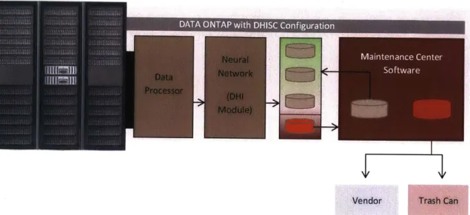
This chapter discusses a new disk failure management pipeline, under which failed disks will be identified in advance and tested prior to being shipped to the Test Site. The goal is to maintain disks while they are still in operation and proactively eliminate "unexpected" failures. DHISC will work alongside SHM [Figure 1] as a messenger between the Disk Layer and the Maintenance Center Software, as shown in Figure 4.

Data Processor

I

I

Shipped via UPS

a UPS

< - Shipped via UPS Spares' Depot

Test Site

-NIY

Figure 4: Our new pipeline for disk maintenance includes a predictive component. DHISC (2, 3, 4) computes the DHI (3) for each disk in the storage system (1). Then it ranks them from the best to worst the disk in the system (4). A system admin can set the threshold for how many of the worst disks should be tested by the Maintenance Center (5) when the

-- -m

The pipeline is shown in Figure 4 and works as follows. Data ONTAP software generates

bi-weekly logs of disk performance as observed from a system-level. DHISC collects the data and

extract time-series information (2). It then feeds it into a pre-trained neural network (3) which

numbers representing disk health for each disk. These numbers are normalized and become the

Dish Health Index (DHI). DHISC then uses DHI to rank disks from least to most healthy. (4) We

envision that whenever the storage system is not experiencing a high number of 1/O requests, the

Maintenance Center will offline the disks ranked near the bottom of the DHISC's rank and test

them, handlingthem as it would pre-failed disks. (5) The number of disks tested would depend on

the threshold selected by NetApp engineers for their customer.

This process can decrease the number of unexpected failures by giving the Maintenance

Center a chance to pre-test disks that might have problems that cannot be detected using the

original thresholding method.

At first, this pipeline can be used just as the one described in Figure 3. However, after this

pipeline proves to be effective within running systems, we can make another simplifying and

cost-saving modification to the disk maintenance pipeline. If the algorithm can identify most the disks

that are going to fail and reduce the number of NTFs (or disks that are failed falsely), it will be more

cost-effective to throw out disks that are marked for failure, rather than to carry them through

Vendor Trash Can

Figure 5: "Trash Can" model to Induce Cost Savings

3.2 DHISC ARCHITECTURE

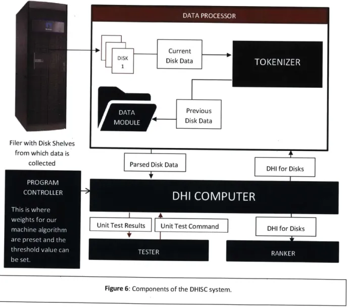
As shown in Figure 4, DHISC has 3 main components: the data processor that processes Data ONTAP system-level disk data into a machine-readable format, the neural network that produces the DHI, and the ranking component that ranks disks according to their DHI and recommends the order in which to maintain the disks in the system. Henceforth, we will refer to these three components as: Data Processor, DHI Computer, and Disk Ranker. The details of this architecture are displayed in Figure 6, and described below.

Data Processor

Data ONTAP outputs bi-weekly system-level data on performance of all its layers [Figure 1]. The Data Processor extracts the disk-related information, handles anomalies in data reporting, and extracts features for the DHI Computer's machine learning algorithm. It consists of a data module and a tokenizer. The data module is a set of files containing disk data - one set for new incoming

data and one set for previously input data. Previous data is augmented with the DHI and exists to

enable quick recovery in case the system is shut down and DHISC loses data. This is necessary

because DHISC uses deltas between two checkpoints to compute certain features for the DHI

Computer. DHISC only relies on having one previous time stamp stored at any point in time. After

data module receives new data point for some subset of disks, it has the tokenizer parse the data

and pass it to the DHI Computer.

DHI Computer

The DHI Computer is the engine of the DHISC system. It contains a pre-trained neural network and

generates a DHI for each disk in the storage system. Chapter 4 gives more details on this process.

Disk Ranker

The last major module is the Disk Ranker. It takes in DHls for all the disks in the system and outputs

an ordered list that can be used by the Maintenance Center to test disks below a certain threshold,

or by an engineer to view the health of the system as a whole. We identify it as a separate module

because it is central to the idea that our definition of good and bad disks is relative.

The remaining program modules improve usability. The Tester Module is responsible for giving the

appropriate inputs and function calls to the tokenizer and the DHI Computer to enable thorough

testing of DHI's functionalities. It is a collection of unit tests that can be accessed via a GUI console

The Program Controller is used to configure the DHI Computer. The DHI Computer is not a deployed neural network. It is pre-trained neural network with predetermined weights and placed into the Program Controller. Likewise, the Program Controller contains data that the Tokenizer uses to parse and compute data for the DHI.

Filer with Disk Shelves from which data is

collected

- Current

DISK _{Disk Data}

-- 1

Previous

0T Disk Data

Parsed Disk Data

DHI for Disks

Unit Test Results Unit Test Command _{DHI for Disks}

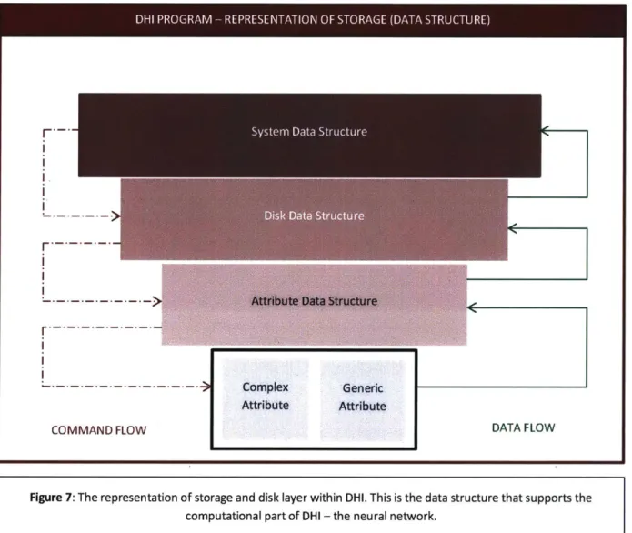
3.3 THE DHI COMPUTER'S LAYERING MODEL

As discussed in the previous section, DHI Computer has two main components: a

representation of disks within the storage system, and a neural network that uses data from this

representation and updated said data. In this section, we describe the representation of disks and

the storage system within the DHI Computer. It is important to have these components, because

they enable us to feed features (pre-processed data from a disk) into the neural network.

---

_>

COMMAND FLOW

Attribute Data Structure

Complex Generic

Attribute Attribute

DATA FLOW

Figure 7: The representation of storage and disk layer within DHI. This is the data structure that supports the computational part of DHI - the neural network.

The storage representation in the DHI Computer is a hierarchy of structures shown in

Figure 7. Each layer of this hierarchy has a set of constructors, destructors, readers, and writers,

which are unique to that layer and rarely propagate up or down to the other layers. The top layer

is all encompassing - it uses features from all the layers that are below it. The chart in Figure 7

displays the hierarchy and flow of commands/information.

At the top is the System Layer. The System Layer keeps track of the number of disks in the

system and the max/min of all attributes it collects for the disks (the attributes correspond to the

data that ONTAP collects about disks at the system level). Below it is the Disk Layer which keeps

track of an array of Disks. Each Disk represents a disk in the storage system and carries data about

its own performance now and in the past, as well as and rates of change in the performance. Each

disk is also responsible for storing (but not calculating) its own DHI.

Finally, the Attribute Layer is a low-level structure for managing Disk attributes.

We will look at each layer of this organization and explain the goal and scope of the layer.

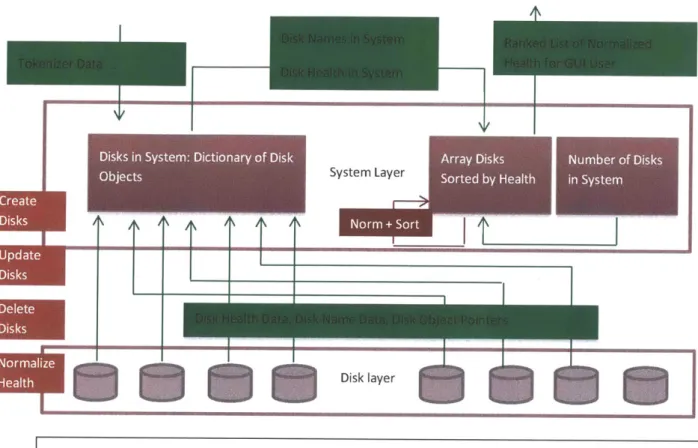
3.3.1 THE SYSTEM LAYER

The Filer - the computer that runs Data ONTAP and manages disks - will ultimately make

decisions on how to maintain the disks, so the System Layer represents the Filer in our software

and contains data necessary to inform disks about their status and to inform the programmer

Disk.s, inl System: Dictionary Of Disk Nurnber of Disks

System Layer

Obet _{in Syste}

Disk layer

Figure 8: The System Layer. Starting from top left, the System accepts data from the Tokenizer and decides

whether to update an existing disk or create a new disk and add it to the Disk Layer. After data updates at the Disk Layer, the System Layer receives a DHI for each disk that it contains. It then normalizes the DHIs and sorts disks according to them.

This System Layer uses the N disk structures created by the Disk Layer to maintain online system status. For example, when the System Layer gets data from the Tokenizer corresponding to some disks, it makes a determination about whether the data belongs to a disk that already exists in the system or a disk that is new to the system. Based on this decision, it tells the Disk Layer whether to create a new Disk object or to update an existing Disk object. The System Layer also takes care of memory allocation to make sure that new disk structures have enough memory space.

The Disk Layer below is responsible for computation of health at an individual disk level,

and so it provides a DHI for each disk forthe System Layer as shown in Figure 8. In turn, the System

Layer computes max and min values of the DHI in the system and uses these values to normalize

the DHI of every disk that belongs to it. Then, it sorts the disks based on their normalized DHI. This

is the Ranker, which will inform the Maintenance Center about the best and worst disks in the

system.

In summary, the System Layer:

* Keeps track of disks that are live and disks that have failed and allocates memory.

" Normalizes DHIs of disks in the system.

* Sorts and outputs disk rank based on their normalized DHI.

3.3.2 THE DISK LAYER

The Disk Layer is responsible for creating, updating, and reading values from Disk

structures. Disk structures maintain pointers to the most current deltas of attributes for that

physical disk, and the health of the disk. The Disk Layer is also responsible for computing the DHI

using a pre-trained neural network. To produce this DHI, the Disk Layer has to pass the data of

every disk through the neural network. Part of this data is a what we call a "Human-Estimated

Moving Average", which is just a moving average of attributes that engineers at NetApp predicted

would correlate with disk failures (see Section 4.3.2). We can treat it just as any other attribute

ourselves at the Disk Layer. The reason we used it is that it improved the neural network performance by 0.6%.

Disk layer

FIILM

Attribute Attrbute

Attribute Layer Attribute Attribute

Figure 9: The Disk Layer. At the top we list all of the functions that the disk layer can perform on the disk data structure. On the bottom we show how the disk attribute layer interacts with the Disk layer above it.

To access all of the other attributes, each Disk has an array of pointers to the attributes in the Attribute Layer. They represent the attributes recorded by Data ONTAP, such as: blocks read, sense errors, etc.

3.3.3. THE ATTRIBUTE LAYER

Attribute Layer is a special layer, because it is a union of two sub-layers. The concept of an

Attribute is generic . For example, 10 latencies are an Attribute, and so are the blocks read and

blocks written. Some Attributes are simple - they have only one value associated with them. For

example, blocks read for a disk is just a count of how many blocks were read. However, there are

other attributes which require heavier computation. For example, 10 latencies are a weighted sum

of many sub-components. The system reports how many 10s are completed within a span of 4ms

and how many 10s are completed within a span of 16ms and the like. 10 latency, however, would

be an aggregate of all those values, more specifically, a weighted sum of all those latencies. This

complex attribute is a combination of simpler attributes, called generic attributes.

The Attribute Layer maintains current and previous values for individual values for

Attributes of disks and expands or shrinks depending on the configuration file given at the

program's start. This layer is generic and easily extendible. To add a new Attribute, the user simply

edits an array of tokens in the program controller. However, the neural network is pre-trained on

a certain data pool, so while the infrastructure can be easilyamended -the neural network needs

to be re-trained if the goal is to include the data into the DHI computation. This data pool is

4.1 OVERVIEW

The "Disk Health Index" (DHI) is a single number that captures information about the likelihood of oncoming disk failure. This value is indicative of the expected time when a disk will fail, but we do not simply treat it as a binary answer. Instead, we use the DHI to rank disks relative to each other, so that we can triage and address disks with highest likelihood of short-term failure first.

The DHI is computed each time that a disk is updated or created within the System in Figure 8, based on a formula pre-determined by a neural network. This formula is a set of weighted sums and function operations. To determine this formula, we first must train the neural network to recognize patterns of disks that would eventually be labeled as failed by NetApp (sent to 3PR) and disks that are performing well. Sections 4.2-4.5 describe the training process.

Because the decision about whether the disk should be labeled Failed by the Maintenance Center, and thus the DHI estimate, depends on the customer, there is no singular definition of disk failure. The DHI - an absolute number - for every disk will be passed to the System Layer, where the System will rank the disks from best to worst-based on the DHI. As such, the DHI presents an absolute predictive metric, and the rank provides an easy way for companies to adapt an absolute metric while retaining flexibility on their definition of disk failure.

Using a rank also provides a-level of comfort to companies that are just introducing neural networks into their products. Neural networks have been popularized only recently, and mostly in research. They have not been around in the industry long enough to generate trust. [26] Having a

relative scale based on the DHI allows companies to have control over the number of false

negatives that neural networks produce. For example, instead of maintaining all of the disks that

the neural network labels as nearing failure, the company may choose to only consider disks for

which neural network shows high confidence. This is useful is because neural networks used for

image recognition have been shown to be fooled with introduction of unexpected noise into the

system to trick the neural network's level of confidence to shift in the opposite direction of the

anticipated and desired prediction [20]. Chapter 6 discusses failure modes in greater detail.

After the DHI runs within real systems at NetApp for some period of time alongside the

existing SHM by adding recommendations via the DHI rank rather than absolute predictions, we

can switch from a relative scale to an absolute predictive metric, if our results on the test set align

with real world results in the field. Chapters 5 and 6 discuss applicability of neural networks in

practice. However, machine learning is, by definition, applied statistics. Machine learning

algorithms are based on using pre-existing data sets to learn patterns of classification to detect

those patterns in novel data sets, and there is an element of unpredictability in using any one of

them, so the relative component is necessary if we are to adapt neural networks in the industry.

The reason we chose neural networks is threefold. First and foremost, the neural network

we trained yielded excellent accuracy with a low rate of false positives. Second, neural networks

and especially deep learning have become popularized [33], and Google recently released a

machine learning library called TensorFlow that focuses on design of neural networks. While we

did not use TensorFlow for our implementation, the fact that TensorFlow exists can enable other

pipelines. There is no barrier preventing another research group or company from implementing

their own neural network to mimic the results of our research. Finally, neural networks are

computationally powerful and flexible. Their structure enables them to fit data well [34], and

changing the structure results in different fits. In contrast, the SVM algorithm, another popular

machine learning tool, requires the use of Kernel transformations to fit the data (33]. At the same

time, neural networks can perform the task of feature selection, if necessary. If another research

group attempts this project with a data set that has many more attributes than ours does, they

can use the technique of auto encoding described in Section 5.2 instead of implementing feature

selection independently [22] (See Chapter 5). Of course, another algorithm can be swapped out

for the neural network. We discuss other alternatives and their performance on our data set in

Section 5.3.

Right now, we are looking at the indices relative to one another, because we do not yet

know what constitutes a bad disk and because the disk maintenance pipeline works well with this

relative model. All a system administrator has to do is decide how rigid of a definition of failure

she wants a system to have, and change the threshold so that all disks with a relative DHI below

the threshold will get tested by the Maintenance Center periodically. Eventually, if we choose to

transition to the Trash Can Model as shown in Figure 5, DHI can be used as an absolute.

This Chapter will show how we compute the absolute DHI that the System later normalizes

and ranks. First, we will discuss the basics of what a neural network is. Then, we will discuss the

structure of the neural network we used, the data that was used for training, and finally - how DHI

4.2 NEURAL NETWORK BASICS

We will first walk through an example neural network to illustrate the basic principles. A neural network is a collection of computational units called neurons, stacked in vertical columns. A neural network takes some matrix as an input and passes it through the layers of neurons, each of which performs some function on its input before it passes the output to the right. The following example mimics Recitation and Lecture materials given by Professor Patrick Winston at MIT [21].

X

W1

W4

Y

W2

Figure 10: A simple neural network which consist of two layers. The first layer contains neurons A and B. The second layer has neuron C. _{Inputs X and Y are both input into neurons A and B. lines represent flow of data.}

Wi-W6 represent weights that are applied to the data flowing through the connecting wire. Each neuron consists of two parts: a summation and a thresholding function. For simplicity, we represent the neurons by its thresholding function, in this case - a step function. Thresholding function can change from one neural network to another. Before inputs entering the neuron are passed through the thresholding function, they are summed together.

Suppose we have two features, one of which is called X and the other is called Y. For this example, X and Y are binary variables. We want to use a neural network so that it tells us for any given value of X and Y, if the output is 0 or 1.

The neural network in Figure 10 consists of neurons A, B, and C. Neurons are functions that, to some extent, mimic how neurons in our brains work. Each neuron contains a summation

(not pictured) which sums all of the incoming weighted inputs, and a thresholding function. A

step function is one such possibility and it happens to be the easiest to visualize, which is why we

use it below. Inputs X and Y take on some values. They are multiplied by weights corresponding

to wires in Figure 10. When weighted X and Y inputs enter the neuron, they are summed and are

then passed into the threshold function. If the summed, weighted inputs exceed the threshold,

the neuron outputs a 1. As the thresholding function is a step function, when an input does not

pass the bar the neuron outputs zero. We provide inputs to each neuron. The first set of neurons

in the neural network are collectively called "the input layer" because they are the first to

encounter the input (in our case - X and Y).

Each line that connects an input to a neuron has a weight on it. W-W6 are weights.

When we give some sample X and Y values to this neural network, the input to neuron A is:

XW + YW3.The input to neuron B is: XW4 + YW2.

The neurons are functions that evaluate if the above input passes the threshold. We

will call the thresholds of the respective thresholding functions TA, TB, and Tc. As a result, the

output for neuron A will be 1 if XW1 + YW3 > TA. The output for neuron B will be 1 if XW +

YW2 > TB.The outputs of neurons A and B will be 0 otherwise. If we take a second look, these

are equations for a line with an indication of which part of the plane to shade as "1" - above the

line or below the line. At the moment, we have two neurons, and each of them produces a line

that divides the X-Y space up according to the neuron A and neuron B inequalities. One of the

sides will be shaded a "1" and the other side will be shaded as a "0". We want this shading to

correspond to the desired output for each X, Y pair. All we know is that based on the initial value

neuron A and one for neuron B based on the weights that it was initialized with: W1, W2, W3, W4, W5, W6.

B A

Y

Figure 11: Each neuron A and B draws a

line in

on

inequality

or

line,

of

of

From the perspective of Neuron C, its inputs are outputs of Neurons A and B. Neuron C's output will be dictated by the following equation:

AW. +.BW6 > Tc

We know that A and B are limited to values 0 or 1. The above equation is a logical operation performed on binary input. This binary input is the shadings in Figure 11. What Neuron

A and Neuron B did to the

X-Y

Neuron B. For example, if Ws = 1 and Ws 1 and Tc = _{1.5, we will get a map of inputs to outputs}

Output of A

_{Output of B}

_{Output of C}

1 1 1

1 0 0

0

₁

₀

0

₀

₀

Table 1: Possible outputs of Neuron C, given all possible values of A and B given that W5 = 1 and W6 = 1 and Tc =

1.5 and identically resembling the AND logical operation.

Under our current assumptions, the neural network would have the picture of the world shown in Figure 12, by applying the AND operation on shadings produced by Neuron A and Neuron B.

A

x

y

Figure 12: Our current assumptions about the neural network in Figure 10 yield a division of the X-Y plane into two regions: one where <x,y> pairs produce output of 0 (non-shaded) and one where <x,y> pairs produce the output of 1 (shaded).