A diffraction integral based turbomachinery noise shielding method

(1)

A Diffraction Integral Based

Turbomachinery Noise Shielding Method

by

Dorian Frederic Marie Colas

Diplome de l'Ecole Centrale Paris (2011)

Submitted to the Department of Aeronautics and Astronautics

in partial fulfillment of the requirements for the degree of

Master of Science in Aeronautics and Astronautics

at the

MASSACHUSETTS INSTITUTE OF TECHNOLOGY

JUL

01

7 _01

LR

BRARIES

June

2011

@

Massachusetts Institute of Technology 2011. All rights reserved.

Author ...

...

Department of Aeronautics and Astronautics

May 19, 2011

C ertified by ...

_{.. , ...}

Zo tin S.

.... .S .o

Spa

k

H. N. Slater Associate Professor

Thesis Supervisor

/

-Accepted by...

...

(

Eytan H. Modiano

Associate Professor of Aeronautics and Astronautics

Chair, Graduate Program Committee

(2)

(3)

A Diffraction Integral Based

Turbomachinery Noise Shielding Method

by

Dorian Frederic Marie Colas

Submitted to the Department of Aeronautics and Astronautics on May 19, 2011, in partial fulfillment of the requirements for the degree of

Master of Science in Aeronautics and Astronautics

Abstract

A current research focus in subsonic aeronautics is the reduction of noise, emissions and fuel burn. The Silent Aircraft Initiative, NASA N+2 and N+3 projects are examples of recent efforts investigating innovative aircraft configurations to meet the future goals of air transportation. This requires novel methodologies to assess unconventional aircraft designs. This thesis is part of the N+2 program and focuses on the development of a method for the assessment of turbomachinery noise shielding in hybrid wing body aircraft.

The preliminary design and assessment of novel aircraft configurations require both low computational cost and versatility of the shielding method. High fidelity methods, such as for example boundary element methods, are computationally expensive and not amenable for optimization framework integration. On the other hand, low fidelity methods, such as the barrier shielding method, are limited in their source and geometry definitions. The diffraction integral method is a simplified ray tracing method capturing edge diffracted rays. Creeping rays and reflected rays are not accounted for making the method suitable for flat geometries with sharp edges. It is based on the Maggi-Rubinowicz formulation of the Kirchoff diffraction theory for monopole source descriptions and is inherently a high frequency method. The diffraction line integral requires numerical integration and does not account for flight effects.

A new method described in this thesis was developed to address these shortcomings. It is based on the Miyamoto and Wolf formulation of the boundary diffraction theory to allow the definition of source directivity inherent to turbomachinery noise. It is amenable to multipole and directional point source descriptions. Bulk flight effects are modelled with a generalized Prandtl-Glauert approach. Computational cost is dramatically decreased using uniform asymptotic theory to reduce the diffraction integral into a simple Fresnel inte-gral. The Fresnel integral is solved via an analytical approximation such that the resulting shielding method does not require numerical integration. The method is applicable to three-dimensional aircraft configurations and comparison with an equivalent source method for sphere and disk shielding test cases show good agreement at high frequencies. Its analytical formulation offers compatibility with optimization frameworks facilitating new perspectives in aircraft design for noise reduction.

Thesis Supervisor: Zoltin S. Spakovszky Title: H. N. Slater Associate Professor

(4)

(5)

Acknowledgments

First, I would like to thank my thesis supervisor Professor Spakovszky for his guid-ance and advice and for challenging me during my two years at MIT. Being part of the MIT N+2 team under his supervision was an honor and a privilege.

I would also like to thank everyone from the GTL. The Professors radically

changed my approach to Fluid Mechanics, Engine Design and, more generally, engi-neering. Also, I could not have completed the project without the students and the open dialog in the lab. Special thanks to my labmate and friend Jeff Defoe for sharing his CFD expertise and Canadianness with me.

MIT would not have been the same without the French crowd and my roommates. You surely contributed to recreating a family far from home.

Thank you to my parents Stephane and Veronique Colas, my sisters Fleur and Laetitia, my brother in law Sebastien for their encouragements, support, and love. I would not have made it here without them and the strong foundation they give to my life. Thank you to my godson Mathis for his smiles and forgiving me for being away most of his first year. I promise that it will pay someday to have a godfather in the US.

Finally, a very special thank you to my love, Lizzy Atkin, for the priceless support she gave me during these years.

(6)

(7)

D.4.1 Find Outline . . . . 110 D.4.2 Calculate Shielding . . . . 110 D.4.3 LSFit... . . . . . . . . . . .. 111 D.4.4 uO... . . . . . . . .. 111 D.5 RunScript... . . . . . . . .. 111 E User Guide 113 E.1 Structure of the Main Folder . . . . 114

E.2 Starting and Running the DIM Code... . . . . . . . . . 114

E.3 Specifying Forward Flight Conditions... . . . . . . .. 114

E.4 Defining the Source Location . . . . 115

E.5 Selecting a Source Model . . . . 115

E.6 Inputting Shielding Objects... . . . . . . . . 117

E.7 Specifying Shieding Object Outline Parameters.. . . . .. 118

E.8 Specifying the Observer Locations... . . . . . . . . . .. 119

E.9 Saving OASPL Pattern . . . . 119

E.10 Exam ples . . . . 120

E.10.1 N2A Example . . . . 121

E.10.2 N2B Example . . . . 121 F Algorithmic Logic 127 F.1 RunScript... . . . . . . . . 127 F .1.1 Inputs . . . . 127 F.1.2 O utputs . . . . 129 F.1.3 Code Logic . . . . 131 F.2 FindOutline.. . . . . . . . 134 F .2.1 Inputs . . . . 134

(11)

F.2.3 Code Logic . . . . F.3 LSFit . . . . F.3.1 Inputs . . . . F.3.2 Outputs . . . . F.3.3 Code Logic . . . . F.4 createuO . . . . F.4.1 Inputs . . . . F.4.2 Outputs . . . . F.4.3 Code logic . . . . F.5 uO . . . . . . . .. F.5.1 Inputs . . . . F.5.2 Outputs . . . . F.6 Code Logic . . . . F.7 CalculateShielding . . . . F.7.1 Inputs . . . . F.7.2 Outputs . . . . F.7.3 Code logic . . . . F.7.4 Subfunction: CheckShadow F.7.4.1 Inputs . . . . F.7.4.2 Outputs . . . . F.7.4.3 Code logic . . . .. F.7.5 Subfunction: Project . . . . F.7.5.1 Inputs . . . . F.7.5.2 Outputs . . . . F.7.5.3 Code logic . . . .. F.7.6 Subfunction: PrepareIntegral F.7.6.1 Inputs... F.7.6.2 Outputs... F.7.6.3 Code Logic . . 11 134 134 134 135 135 137 137 137 137 140 140 140 140 140 140 141 141 142 142 142 143 143 143 144 144 144 144 144 145

(12)

F.7.7 Subfunction: Integrate . . . . 146

F.7.7.1 Inputs . . . . 146

F.7.7.2 Outputs . . . . 146

(13)

List of Figures

1-1 NASA goals for the next generations of aircraft [11].. . . . . 24

1-2 SAX-40 Conceptual Aircraft Design [21. . . . .

24

1-3 Boeing N2A (top) and N2B (bottom) configurations based on the cargo

version of the SAX- 40 and using podded and embedded engines re-spectively [picture courtesy of D. Odle, Boeing]. . . . ... 26

1-4 HWB aircraft acoustic shielding comparison between: a) barrier shield-ing method [3], b) diffraction integral method [3], and c) ray tracshield-ing

m ethod [4]. . . . .

28

1-5 Schematic of the different rays involved in Ray Tracing Methods: In-cident, reflected, edge diffracted and creeping rays. . . . . 29 1-6 Schematic of the equivalent sources defined on the surface of the

shield-ing object in a boundary element method [3]. . . . . 30 1-7 Schematic of the equivalent sources defined on the surface of the

shield-ing object in a Equivalent Source Method [3].

. . . .

31

2-1 Formulations, challenges and solutions in the DIM derivation. .... 36

2-2 Relation between shielding geometry, source and observer locations 37 2-3 Control volume definition . . . . 39

2-4 Boundary conditions corresponding to the Kirchoff diffraction theory. 40

2-5 Control volume description for the Maggi and Rubinowicz formulation. 41 2-6 Strategies to evaluate the diffraction line integral. . . . . 44

2-7 Evaluation of the Fresnel integral F[x] and its asymptotic expansion. 48

(14)

2-9 Illustration of the two transformations: real part of the pressure

radi-ated by a monopole acoustic source in a uniform background flow (M = 0 and M =0.3). a) without flight effects, b) Taylor transformation and c) Generalized Prandtl-Glauert approach. . . . . 55

2-10 Relative difference between the Taylor transformation and the gener-alized Prandtl-Glauer approach in the case of a monopole source in a uniform background flow for various Mach numbers square M2 and

reduced frequencies kr...

. . . .

. . . . .

56

3-1 Comparison of the polar directivity patterns (in dB) in the far field

(kr = 1000) obtained with the ANOPP fan module, the corresponding

HELS field reconstruction and directional point source. Left: 50 Hz.

R ight: 10000 Hz. . . . . 62 3-2 Maximum deviation (in dB) in free field between a directional point

source description and the corresponding HELS reconstruction. . .. .. 62 3-3 Left: noise attenuation pattern comparison: directional point source

vs HELS description for a HWB aircraft configuration.

Right: distance between outline points and the source location. ... 63

4-1 DIM structure for integration with ANOPP... . . . . . . . . . . 66

4-2 Parametrization of geometry for implementation of the diffraction in-tegral m ethod. . . . . 68 5-1 Shielding sphere and disk configurations for the validation of the

Diffrac-tion Integral M ethod. . . . . 72 5-2 Disk (Left) and Sphere (Right) shielding comparisons between DIM

and FSC at ka = 92, 194 and 400. . . . . 74

5-3 Disk shielding comparisons between DIM and FSC at ka = 1 (left) and

ka = 50 (right)... . . . . . . . 75

(15)

5-5 N2A aircraft configuration attenuation patterns (in dB) for a) monopole, b) dipole description, and c) HELS directional point source description. 77 5-6 Difference in insertion loss (in dB) - monopole vs HELS directional

point source.. . .. . . .. . . . . 79 5-7 Difference in shielding (in dB) relative to static conditions for a forward

flight Mach number of

M

0 = 0.2 using a monopole source.

D-1 Diffraction Integral Method v2.00. . . . . D-2 Code flow chart. . . . .

E-1 E-2 E-3 E-4 E-5 E-6 E-7 E-8 . . . . 80 102 103

Polar angle definition.. .... ... Spherical coordinates .. . . . .

N2A geometry... . . . ..

Screen captures, N2A example, inputs. Screen captures, N2A example, outputs.

N2B geometry... . . . ..

Screen captures, N2B example, inputs. Screen captures, N2B example, outputs.

. . 117 . . . . 120 . . . . 121 . . . . 122 . . . . 123 . . . . 124 . . . . 125 . . . . 126

F-1 DIM v2.00: Code Flowchart. . . . . F-2 Indices on problem geometry. . . . .

F-3 Coordinate systems (top: spherical, bottom: cartesian).... . ..

F-4 Analytical expressions [5] of the first a) associated Legendre functions and b) spherical Hankel functions. . . . . . . . ..

128 128 130

(16)

(17)

List of Tables

1.1 Capabilities and drawbacks of current noise shielding methods. ... 27

(18)

(19)

Nomenclature

Abbreviations

ANOPP Aircraft NOise Prediction Program

BEM Boundary Element Method

BDWT Boundary-Diffracted Wave Theory

BWB Blended-Wing-Body

CMI Cambridge-MIT Institute

DIM Diffraction Integral Method

ESM Equivalent Source Method

GO Geometrical Optics

GTD Geometrical Theory of Diffraction

HELS Helmholtz Equation Least Square FAR Federal Aviation Regulations

FSC NASA's Fast Scattering Code for noise shielding prediction

HWB Hybrid-Wing-Body

N2A Hybrid-wing-body aircraft with conventional podded engines

N2B Hybrid-wing-body aircraft with embedded propulsion system

OASPL Overall Noise Attenuation Sound Pressure Level

PG Prandtl-Glauert

RTM Ray Tracing Method

SAI Silent Aircraft Initiative

SAX Silent Aircraft eXperimental design

SPL Sound Pressure Level

(20)

Roman Symbols

A _{area of integration} _(im2 ) a shielding sphere radius (in)

co speed of sound (m.s 1

)

C j-th coefficient in HELS noise description (Pa)

f

amplitude of harmonic integrand (Pa.m-1) g phase function (M)

H monopole source strength (Pa.m)

Ir integral of acoustic pressure potential along a linear edge (Pa)

k _{wavenumber (m-1)}

L length of contour of integration (m)

M

0 flight Mach number

p acoustic pressure (Pa)

Pd boundary-diffracted acoustic pressure (Pa)

pA incident acoustic pressure without diffraction (Pa)

Po amplitude of incident monochromatic acoustic pressure (Pa)

Ps scattered acoustic pressure (Pa)

Q

directional point source strength (Pa.m) r vector from observer to outline location (m)

r magnitude of r' (m)

R vector from source to obsever (m)

R magnitude of R (m)

s

curvilinear abscissa (m)

t detour parameter for end-points (in)

V fluid velocity (m.s1 )

X transformed location relative to aircraft (m)

W acoustic pressure potential (Pa.n-1

)

YO

initial point of linear edge

x, y, z coordinate system relative to aircraft: x = aft, y starboard, z up x1, yi, zi transformed coordinate system relative to aircraft

(21)

Greek Symbols

O

polar angle (rad)

3 _{distance between point and line defined by a linear edge (in)}

O

polar angle (rad)

rK _{transformed wavenumber (m-}1₎ { coordinate in transformed domain (m)

( _{detour parameter for stationary phase point (n)} A wavelength (m)

p _{vector from source to outline location (M)}

p magnitude of i (m)

p density (kg.m-3)

0 azimuthal angle (rad)

4

acoustic velocity potential (m2 _.S-1)

o _{amplitude of acoustic velocity potential (m2} _-1₎

<D velocity potential divided by the uniform mean flow speed (m)

(22)

(23)

Chapter 1 Introduction

Reducing noise around airports while decreasing fuel burn is one of the challenging goals of current research in aeronautics. In response to the growth of air transporta-tion, NASA and other government agencies are funding research to address these challenges.

Funded by the Cambridge MIT Institute (CMI), the Silent Aircraft Initiative

(SAI) investigated unconventional aircraft designs which could potentially be both

fuel efficient and of low noise signature. The effort resulted in a promising Hybrid-Wing Body (HWB) aircraft configuration dubbed the SAX-40 (shown in Figure 1-2

[2]). Utilizing a large lifting planform area to shield the noise generated by the turbo-machinery along with advanced operational procedures, the SAX-40 was calculated to achieve 61 dBA with a 25% reduction in fuel burn

12].

NASA's N+2 program focuses on reducing both noise and fuel burn. In this case, the NASA goals are set for the second generation of aircraft beyond the one currently in service. To address the challenges related to the growth of air transportation, they goals shown in Figure 1-1 need to be met by further aircraft design.

The N+2 project requires medium fidelity methodologies with the ability to assess the potential of innovative designs. These methods also need to be fast, in order to allow the investigation of a broad design space (see for example [2]).

(24)

N+01X2015* N+2.202"* N+3 a202**

TechnologyBm RelsUv TaecnologyBends Relative Tcholoy Bwn

To

a

nge

confiuaton

Asle RO

i

renc

e

Ta

e____I_ co__o

LargeTdInAW* e

Noise

(cum below Stage 4) -32 dB -42 dB -71 dB

LTO _belowNO, Emi _{CAEP 6)}

-60%

-75%

better than -75%

__ _ _ _ _ _ __ _ _ _ _ _ __ _ _ _ _ _ _ _ _

PerlomnancC

MOMa Fu Bum -33%**

-50%**

better than -70%

-33%

-50%

exploit metro-plex* concepts

Figure 1-1: NASA goals for the next generations of aircraft [1].

Figure 1-2: SAX-40 Conceptual Aircraft Design [2].

(25)

1.1 NASA's N+2 Subsonic Fixed-Wing Project

One of the main objectives of the N+2 project is to develop methodologies for the de-sign of quiet, fuel-efficient aircraft. These methods must be compatible with advanced and unconventional configurations.

The N+2 project is divided into two phases and the high-level tasks of the program lead by the Boeing-MIT-UCI team are briefly summarized.

Phase I

" Definition of a non-proprietary HWB aircraft configuration based on a cargo

conversion of the SAX-40 to be used as a platform for assessment of methods and technologies developed during the project.

" Expension of the design for two different propulsion systems (see N2A and N2B

configurations in Figure 1-3).

" Initial noise and fuel burn assessment of the aircraft.

" Planning of the aero-acoustic and aerodynamic wind tunnel test.

Phase II

" Improvement of existing prediction methods for the design and analysis of

un-conventional HWB aircraft that meet the N+2 goals at no computational cost increase.

* Refinement of the candidate HWB aircraft to meet the N+2 goals.

" Fabrication of the HWB aircraft model for the wind tunnel test.

" Validation of the prediction methods with aero-acoustic and aerodynamic test data.

The goal of MIT's phase II effort was to develop prediction methods to be imple-mented into NASA's Aircraft NOise Prediction Program (ANOPP). ANOPP assesses

(26)

Figure 1-3: Boeing N2A (top) and N2B (bottom) configurations based on the cargo

version of the SAX- 40 and using podded and embedded engines respectively [picture

courtesy of D. Odle, Boeing].

the different aircraft noise contributions and executes a Federal Aviation Regulation

(FAR) Part 36 certification estimate (see [6]). The current methods implemented

in ANOPP (see Heidmann Fan module [7] for example) are based on correlations of

experimental data and are of low computational cost. A key limitation is that they

are based mostly on conventional aircraft configurations. The challenge for the new

methods is to be of applicable to alternative configurations at no computational cost

increase.

MIT's task was to develop an alternative to ANOPP's method for turbomachinery

noise shielding assessment. ANOPP currently employs the barrier shielding method

derived from the work of Beranek [8] and Maekawa

[9]

(see description in next section).

The effort led by the University of California Irvine aimed at the development of

a jet noise shielding methodology [10]. The objective was to improve on the barrier

shielding by a higher fidelity method that does not require a dramatic increase in

computational ressources.

(27)

1.2 Current Shielding Methods

There are four main classes of shielding assessment methods which can be used for noise shielding prediction. For integration into ANOPP, the new method should be of higher fidelity and flexibility than the Barrier Shielding Method but at no com-putational cost increase. These requirements and the following comparison between current methods summarized in the next sub-sections motivated the development of the Diffraction Integral Method. As seen in Table 1.1, higher fidelity methods require a dramatic increase in computational ressources.

Table 1.1: Capabilities and drawbacks of current noise shielding methods.

Computation Source Flight

-al cost directivity effects

Ray tracing High ++ No 3D Yes

method

BEM High +++ Monopoles, 3D Yes

Dipoles

ESM High +++ Multipoles 3D Yes

Barrier shielding Low - _No _2D _No

method

DIM Medium - Any 3D Yes

1.2.1 Barrier Shielding Method

Beranek [81 and Maekawa

19]

developed a barrier shielding method based on empirical correlations of noise attenuation to Fresnel's number for a semi-infinite rectangular screen. The method therefore considers only straight edge diffraction from planar shielding geometries. Furthermore, it does not account for source directivity and flight effects. Although it is computationally inexpensive, the above-mentioned limitations are prohibitive for its use in turbomachinery noise shielding prediction of complex 3D configurations. Figure 1-4 illustrates the application of the barrier shielding method to a hybrid wing body aircraft.

(28)

AdB 40,

-40

-20 0 -20 -40 -60 -400-20 Longitudinal Distance (m)

a) Barrier shielding method

0 20 40 60

Longitudinal Distance (in)

b) Diffraction integral method

8SPL' -9.6 12.7 16A -19.0 -25.3 -28.4 -31.6 x (M)

c) Ray tracing method

Figure 1-4: HWB aircraft acoustic shielding comparison between: a) barrier shielding

method [3], b) diffraction integral method [3], and c) ray tracing method [4].

(29)

observer

incident ray

noise source """"" Pay '" ' creeping ray

s

ielding

object

Figure 1-5: Schematic of the different rays involved in Ray Tracing Methods: Incident,

reflected, edge diffracted and creeping rays.

1.2.2 Ray racing Methods

These methods are based on a high frequency approach. Geometrical optics is applied

to compute the field due to incident and reflected rays on the shielding object. The

Geometrical Theory of Diffraction provides the necessary extension to evaluate the

acoustic field in the shadow regions. It introduces diffracted rays in addition to

reflected and refracted rays encountered in the classical geometrical optics. There are

two types of diffracted rays: edge-diffracted rays and creeping rays, as illustrated in

Figure 1-5.\Ray Tracing methods are generally setup for monopole noise sources and

are computationally expensive since the path of each ray needs to be evaluated with

an iterative scheme. These considerations limit their use for noise shielding prediction

and integration into ANOPP. But the accurate modeling of noise scattering by ray

tracing methods and their compatibility with flight effects at low Mach numbers (as

a first order approximation such as described in

[4])

makes them amenable for noise

shielding assessment in the more advanced design stages. Van Rens [11] demonstrated

applicability of the ray tracing method to complicated shielding geometries such as

Blended Wing Body aircraft configurations. During the Silent Aircraft Initiative,

Agarwald and Dowling [4] quantified acoustic shielding effects of a Hybrid Wing

Body aircraft by a ray-tracing method (see

[4])

and found that the frequencies from

the noise spectrum of the propulsion system were sufficiently high for ray theory to

yield results that compared well with experiments.

(30)

1.2.3 Boundary Element Methods

surface point sources

noise source

observer

_shielding

_object

Figure 1-6: Schematic of the equivalent sources defined on the surface of the shielding

object in a boundary element method [3].

In the case of noise scattering computations, boundary element method (BEM) codes

are solving for an integral version of the Helmholtz equation. The solution at any point

in the computational domain is represented by an integral over the outer-boundary.

By representing the boundary edges as a set of panels or 'equivalent sources', as

il-lustrated in Figure 1-6, the boundary integral equation is reduced to a linear system

of equations making a numerical solution possible. Solving the linear system can

be-come computationally expensive as the matrix size depends on the size of the shielding

object and the mesh which should be fine enough to resolve the relevant source

fre-quencies. Also, the problem reduction into a panel method is valid for monopoles

or dipoles only. Because of the mentioned computational requirements, boundary

element methods are likely not preferred for integration into ANOPP. Assuming the

mesh size to be smaller than the wavelength, the BEM methods are more accurate

than the barrier shielding and ray tracing methods, applicable to complex shielding

geometries at any source frequency. As such, they have been used for acoustic

shield-ing prediction of Blended Wshield-ing Body aircraft configurations. Durshield-ing the previously

mentioned SAI program, Agarwald and Dowling [12] developed a BEM code

account-ing for flight effects usaccount-ing the transformation suggested by Taylor [13] and applied it

for noise shielding assessment of the SAX-03 airframe. As computational cost became

impractical at high frequency, the analysis was carried at a reduced frequency ka of

50, where k is the wavenumber and a is the center body chord equivalent to a full

(31)

scale frequency of 50 Hz. This low frequency noise attenuation assessment revealed

a potential shielding of up to 18 dB by the considered airframe.

1.2.4 Equivalent Source Methods

point sources on . -g -

noise

source

auxiliary surface

e'

observer

-shielding object

Figure 1-7: Schematic of the equivalent sources defined on the surface of the shielding

object in a Equivalent Source Method [3].

Equivalent source methods are based on the same approach as boundary element

methods. Both methods express the acoustic field in terms of equivalent source

con-tributions. While in the boundary element method case the equivalent sources are

located on the boundary of the shielding object and are either monopoles or dipoles,

the equivalent sources are located inside the structure as illustrated in Figure 1-7.

This enables the sources to be of multipole nature (monopoles, dipoles, quadrupoles,

etc.). Similar to boundary element methods, solving the linear system of equations

can rapidely make equivalent source methods impractical at high frequencies.

An example of the equivalent source method is NASA's Fast Scattering Code

(FSC) that computes the scattered acoustic field produced by the interaction of an

incident sound from a known noise source with a body of arbitrary geometry. Reimann

et al. [14] validated the Fast Scattering Code on realistic shielding object shapes by

carrying out numerical studies on the scattered noise field surrounding a blended

wing body center nacelle and comparing the results with experimental data. Good

agreement between experimental results and simulations indicated that the FSC is

able to predict the acoustic behavior of the source plus center nacelle combination.

Dunn and Tinetti [15][16] derived and implemented a generalized Prandtl-Glauert

(32)

transformation for NASA's Fast Scattering Code to account for flight effects. They demonstrated the code's ability by applying it to cases involving model nacelle, wing, and airframe components.

1.3 Previous Work

Most turbomachinery noise shielding assessments of advanced aicraft configurations such as HWB-type configurations have been studied using either ray tracing, bound-ary element method or equivalent source method codes. As shown in Table 1.1, none of these methods offers the required combination of medium fidelity, flexibility and low computational cost to be an improved alternative to the barrier shielding method. Furthermore, these methods cannot be integrated into optimization frameworks where a large number of aircraft configurations is explored.

This consideration motivated the development of a simplified ray tracing method, called the Diffraction Integral Method, to meet the objectives and goals of the N+2 program [3][171. The original version was based on the Kirchoff theory of diffrac-tion which is derived assuming the incident acoustic field to be unchanged on the surface of the shielding object. This approximation holds when the wavelength is much smaller than the shielding object and is therefore limited to high frequencies. Since turbomachinery noise frequencies are high, the diffraction integral method is deemed adequate to assess FAR 36 noise. In comparison to ray tracing methods, an inherent shortcoming of this approach is that its underlying theory captures only edge-diffracted rays. Also, flight effects are not accounted for.

This original version of the diffraction integral method makes use of the Maggi-Rubinowicz potential [181 to reduce the Kirchoff diffraction surface integral into a line integral along the outline of the shielding object. The outline is determined based on the source line-of-sight. Although this transformation reduces the computational cost, it also inherently constrains the source to a monopole description. The resulting line integral is then expressed in a form that can be integrated numerically using an adaptative Gauss-Kronrod quadrature method as suggested by Lummer [19]. The

(33)

cal shielding geometries: a sphere and a circular disk. It was shown to perform better at high frequencies and for disk-like geometries.

To summarize, the original version of the diffraction integral method is simpler than higher fidelity methods with the inherent limitations given the involved concepts that (1) the diffraction pattern is characterized by edge-diffracted rays only, (2) the reduced frequency is assumed high, (3) the acoustic source is a monopole, (4) flight effects are not accounted for, (5) a numerical integration scheme is required.

1.4 Thesis Objectives and Goals

The underlying idea of this thesis is to use concepts from the field of optics with the goal to model noise scattering for arbitrary source descriptions at low computational cost.

More specifically, the thesis objectives are to: (1) reformulate the approach of the original version of the Diffraction Integral Method to be amenable to various source descriptions and to account for flight effects, (2) demonstrate applicability to wide range of geometries and validate the method against a high fidelity method and, (3) decrease computational cost of the diffraction integral method to be compatible with

ANOPP and optimization frameworks.

1.5 Thesis overview

The next chapter reviews the theory of boundary diffracted waves and explains the key ideas and concepts behind the derivation of the diffraction integral method. Chapter

3 assesses the error due to the use of a directivity function to include directivity in the

noise source description. It can be concluded that this approach should be avoided in the case of turbomachinery noise shielding assessment. Chapter 4 explains the implementation strategy of the method. The last chapter describes the validation of the diffraction integral method through comparisons with NASA's FSC and delineates

(34)

its limitations. It also illustrates the application of the method to the N2A aircraft configuration and investigates the impact of source directivity and flight effects on the noise attenuation patterns.

1.6 Contributions

A new high frequency approach for the diffraction integral method has been

formu-lated to remedy to limitations of the original method. The enabling concepts bor-rowed from the geometrical theory of diffraction allow the use of source descriptions such as monopole, dipole and directional point sources. The obtained expression for the diffracted pressure field is reduced to a simple expression involving Fresnel inte-grals, which can be approximated analytically. Therefore, and unlike higher fidelity methods such as the boundary element method and the equivalent source method, the diffraction integral method does not require the use of a numerical integration scheme. This reduces the computational cost dramatically. The diffraction integral method accounts for flight effects using a generalized Prandtl-Glauert transformation. It is compatible with alternative aircraft configurations similar to the original method. The new method is therefore of higher flexibility and fidelity than the currently used barrier shielding method at no computational cost increase. The new method is in the process of being implemented in ANOPP.

Turbomachinery noise shielding assessment of the N2A airframe using the diffrac-tion integral method revealed a difference in attenuadiffrac-tion pattern of up to 12 dB between a directional point source and a monopole point source. The forward mo-tion of the source and the N2A airframe was also shown to modify the insermo-tion loss pattern of up to 2.5 dB compared to a static case.

(35)

Chapter 2 Theoretical Derivation of the

Diffraction Integral Method

This chapter outlines the derivation of the expression for the scattered-noise around an arbitrary object at a given forward flight condition as implemented in the Diffraction Integral Method. The diffraction integral method is based on the Kirchoff diffraction theory [181 that expresses the diffracted field at any point as the superposition of waves emitted from the aperture through which the incident field is diffracted. Formally, the scattered field can be written as a surface integral on the aperture area.

Evaluating the diffraction surface integral numerically can become computation-ally expensive for high frequencies and large objects as the number of points required

by the numerical scheme scales with the area of the object and square of the source

frequency to resolve the wavelength of the sound. To reduce computational cost, the Kirchoff diffraction surface integral is transformed into a line integral, discretized and evaluated analytically under the assumptions outlined in the next-subsections.

2.1 Conceptual Summary

Turbomachinery noise frequencies are sufficiently high such that concepts from the field of optics can be applied for turbomachinery noise shielding assessment. The high frequency assumption will be tested and validated in Chapter 5 for the frequencies of

(36)

Step Formulation Challenge Solution

1. Kirchoff diffraction Computationally Miyamoto and Wolf surface integral expensive: N % k'A transformation

2. Diffraction line integral Computationally Analytical evaluation 2 along aperture edge expensive: N -k L with asymptotic theory

Analytical expression _{Complementary}

3. for diffraction through geometry of interest Babinet's principle aperture

Analytical expression Account for flight

4. for diffraction around effects with previous Generalized

Prandtl-shielding object thoyGlauert transformation

Expression for scattered field around object accounting for

flight effects

Figure 2-1: Formulations, challenges and solutions in the DIM derivation.

interest.

Key enabling concepts from the Geometrical Theory of Diffraction [20] are there-fore used in the following sections to derive the desired formulation for the scattered pressure. The required steps, challenges and solutions are illustrated in Figure 2-1, where k is the wavenumber, A is the area of the shielding object are and L is the length of the edge of the object.

The noise attenuation due to shielding can then be calculated as the ratio of the total acoustic pressure to the incident acoustic pressure:

ASPL = 20logi Ps = 20log1o A + Pd (2.1)

Pi Pi

where ASPL is the insertion loss due to shielding in AdB, ps the scattered field around the object, pi the incident field and Pd the boundary diffracted field.

(37)

P

-

_-_-_-_--_ Screen with aperture A

P (observer)

Figure 2-2: Relation between shielding geometry, source and observer locations

The overall noise attenuation can be summed over all frequency bands according

OASPL

=10log10

Z

10 (2.2)

The next sections outline each of the previous steps illustrated in Figure 2-1.

2.2 Diffraction Theory

As mentionned above, the diffraction integral method is based on the Kirchoff diffrac-tion theory and its corresponding surface integral. A possible strategy to evaluate this surface integral is to use a numerical integration scheme. However, the mesh used in the integration scheme must be fine enough to resolve the sound wavelength at their respective frequencies. Therefore the number of required points, N, scales as

N oc k2A where k is source wavenumber and A is the area of integration. At high

frequencies and for large objects, the computational cost associated with numerical integration is limiting. A transformation of the diffraction surface integral into a line integral along the outline of the shielding object is therefore used. This section outlines the first step in the conceptual summary of Fig. 2-1.

(38)

2.2.1 Kirchoff Diffraction Theory

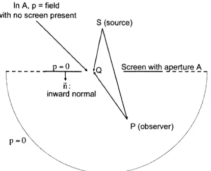
Consider the shielding geometry illustrated in Figure 2-2: an acoustic point source

S and an observer P are separated by a solid screen with an aperture A. The scalar

field emitted by the source in the abscence of the screen, p, is known a priori. Both the scalar fields ps and pi follow the Helmholtz equation outside of the surface of the screen and the source location:

Aps

+

k

2 _ps

₌

₀

(2.3)

Ap,

+ k2p, - 0,

where k is the wavenumber.

Applying the Gauss and Green theorems on the control volume C1 drawn in Figure 2-3, Eq.(2.3) can be re-written as

1 Q)_ eik?- eikr

ps(P) = s(Q)-V - - er .Vps(Q) dS. (2.4)

4iraci

r

*sQj

To simplify the previous expression and to obtain an explicit expression for ps, Kirchoff introduced the following boundary conditions on the control volume:

*

ps = 0 on the screen (hard boundary condition)

e ps 0 on the spherical surface enclosing the volume (far enough from the

source)

*

ps = pi on the aperture.

The first condition states that the shielding object is at rest and non-oscillatory i.e will not emit noise. This is valid for solid objects with resonance frequencies different than the source frequency. The second condition states that far from the source the energy is spread out and the pressure field is zero.

The last condition is an idealization to the real field distribution by assuming that the incident field is unchanged by the screen. It is valid at high frequencies

(39)

Screen with aperture A

5:

inward normal

P (observer)

'

Control

o-volume (C

1

)

Figure 2-3: Control volume definition

for wavelengths small compared to the aperture size. These boundary conditions are summarized in Figure 2-4.

Substituting the previous boundary conditions into Eq.(2.4), only the part of the integral on the aperture remains and the Kirchoff surface integral can be deduced:

1 e ikr eikr

Ps(P) = -PQ) V- - - -Vpi(Q) dS. (2.5)

47rfA[P Q r r

2.2.2 Theory of Boundary Diffracted Waves

To simplify the Kirchoff surface integral, the contributions of the incident geometrical optics field and that of the boundary-diffracted field are identified by the theory of boundary diffracted waves. The geometrical optics field, denoted as PGO, is the undis-turbed incident wave in the illuminated region, which passes through the aperture without interacting with the edge discontinuity. The remainer of the surface integral is the boundary-diffracted wave, denoted Pd, which is formed by the interaction of

(40)

In A, p = field

with no screen present

S (source)

p =

0 Scr

inward normal

een

with aperture

A

P (observer)

Figure 2-4: Boundary conditions corresponding to the Kirchoff diffraction theory. the incident field with the edge. Formally, this can be written as

ps(P) = PGO(P) + Pd(P)

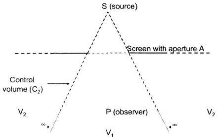
where pGO(P) pi(P)X(P) and X(P) is the unit step function equal to one when P

is inside V1 and zero when P is inside V2 (see Figure 2-5).

Since the BDW depends only on the outline of the shielding object, it can be expressed as a line integral as discussed in the next sub-sections.

2.2.2.1 The Maggi and Rubinowicz Potential

In the case of monopole source descriptions, Maggi and Rubinowicz {21][22] expressed the boundary diffracted wave field as follows.

Consider the control volume C2, drawn in Figure 2-5 which is composed of the aperture A and the lateral surface of the truncated cone B, defined by rays originating from the souce and directed towards points on the edge contour of the aperture. Using

(2.6)

(41)

/ \ / \

/ \

/\

_ _

----

creen

with a

erture A

Control

volume (C2)

V

2

P

(observer)

V

2

VI

Figure 2-5: Control volume description for the Maggi and Rubinowicz formulation.

the Gauss and Green theorems on C2 results in

1 eikr ikr

pni-V

- er -VpJ dS = PGO(P)- (2-7)

47 fac2=A+B r r

Substituting the scattered field expression given by the Kirchoff surface integral in

Eq. (2.5) in the previous expression, and using Eq. (2.6), the boundary diffracted wave

is given as

1 eikr

eikr-pd(P)

=

pnf-V--

--- -Vp

dS.

47f f r r

ik

Assuming a monopole source description i.e pi(Q) = H , where H is the source

strength, Maggi and Rubinowicz derived an analytical expression for the above equa-tion. This can be written in terms of a line integral along the contour C of the

aperture:

Hf eikpeikr -X r~) -ds

pd(P) = - P . (2.8)

47F

C p

r pr +p-r

2.2.2.2 The Miyamoto and Wolf Potential

Extending the work of Maggi and Rubinowicz by making use of vector algebra, Miyamoto and Wolf [23][241 showed that the expression in Eq.(2.8) is also exact

(42)

for oblique plane waves. Further, they showed that if the incident wave is neither plane nor spherical, the same potential holds as the leading term of an asymptotic expansion involving inverse powers in

k

and becomes

1

f

(Peikr

(-5x

j?) di

Pd(P)

-

Tp_'p

P

..

(2.9)

4zr C

r pr +p -r

In the following developments, the diffraction potential will be denoted W and the previous expression can be written simply as

Pd(P) =

fW

-d. (2.10)

2.2.2.3 Singularity in the Diffraction Potential

The line integral is an exact form as derived by a rigorous integration of the surface integral along the shadow boundary. It is non-uniform since the integrand approaches infinity in the so-called transition region where pr + p- r = 0. This region, where the potential diverges, corresponds to observer locations where x transitions from 1 to

0. As a consequence of the discontinuity of the geometrical optic field in this region,

the integrand becomes singular to compensate for this discontinuity and to ensure continuity of the overall scattered field.

This non-physical singularity is a limitation of the boundary diffracted wave theory

[25][22]. Lummer [191 introduced a means to subtract it from the computational domain and gave an explicit form for its contribution to the scattered field. However, the expression he developed holds only for the Maggi and Rubinowicz formulation, i.e. in the case of a monopole source description. It will be avoided using the Uniform Theory of Diffraction as illustrated in the next sections.

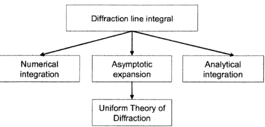
2.3 Discretization of the Integration Contour

To obtain an explicit expression for the diffraction line integral (Eq.(2.9)), the contour of integration is discretized into linear edges {FI}. Thus the problem is reduced to

(43)

next sections outline the derivation of such an expression. Knowing this expression, the diffracted field can then be computed by superimposing the contribution of each

linear edge according to

Pd(P)

=j

-ds~Z

W

- ds.

(2.11)

In practice, the level of discretization is decreased until no differences are observed in the obtained noise attenuation patterns.

2.4 Uniform Asymptotic Expansion of the Line

In-tegral

Although computational cost has been decreased by reducing the Kirchoff diffraction surface integral (Eq.(2.5)) into a line integral as in Eq.(2.9), the number of points required to evaluate the scattered pressure scales with kL with L the length of the contour of integration. Again, computational cost associated with numerical inte-gration can become prohibitive for high frequencies and large objects. In the case of monochromatic waves, asymptotic theory offers a simple way to express Eq.(2.9) analytically on a linear edge and to avoid the use of a numerical integration scheme. However, it introduces spurious singularities as a result of the loss of information. The Uniform Theory of Diffraction [26] is used to avoid these singularities by re-expressing the expansions in terms of Fresnel integrals, which are continuous distributions.

2.4.1 Monochromatic Source Description

The case of a compact, monochromatic wave is considered throughout the following derivations. It can be written as

(44)

Figure 2-6: Strategies to evaluate the diffraction line integral.

where po(p is the wave amplitude.

Po(p can describe any arbitrary compact and monochromatic wave such that pi (p)

satisfies the Helmholtz equation (see Eq.(2.3)).

2.4.2 Line Integral Formulation for the Application of

Asymp-totic Theory

Consider an arbitrary linear segment F characterized by a unit vector e, an initial point o and start and end points denoted by their curvilinear abscissae sa and sb.

Making use of the compact source description (Eq.(2.12)), the diffraction line integral along F, Ir,, can be re-written as a Fourier integral

Ir

= -

dJ=

f

V

1 (P

p- xr)

dieik(r+p)

_ (5)eikg(s)ds,

(2.13)

Jr 4 Jr r J+r-r jr

where

f

and g are the amplitude and phase functions of the integral respectively. The harmonic nature of Ir and its singularity in the transition region renders nu-merical integration inaccurate and computationaly expensive since it requires adap-tive integration schemes. In simple cases analytical solutions can be derived (see for example [27]). An alternative way of evaluating Ir is offered by the asymptotic expansions theory and the method of stationary phase [28]. These strategies are investigated here. Figure 2-6 illustrates the possible solution paths.

(45)

2.4.3 Asymptotic Expansions and Method of Stationary Phase

If the phase function g does not have any stationary phase points inside r (i.e Vs

C

F, g'(s) f 0), the asymptotic expansion of integral in Eq.(2.13) can be obtained via integration by parts:

Ir f b f (s)eikd 1

F-

f(sb) eik(Sb)

f(s)

eikg(s) + 0(k-1). (2.14)

s ik _g'(sb) 9'(sa) (

In this case, the integral is governed by its end points contributions. For a monochro-matic wave, the phase function is g(s) = r(s) + p(s) and the linear segment has a stationary phase point if there exists a point where the total distance r + p is minimal.

On the contrary, if g has one stationary phase point of order 2 lying on F at the abscissa s* such that g'(s*) = 0 and g"(s*) = 0 then the evaluation of the integral is governed by its stationary phase point contribution. The method of stationary phase

[28] gives an explicit expression according to

Ir = 4f (s k"s eikg(s*) + 0(k-1/2_). _(2.15)

2

f

kg~ /~I(s

Depending on the stationary phase point location, either Eq.(2.14) or Eq. (2.15) is taken into account. A drawback of this approach is the introduction of a singularity

in the contribution of the end-points. When the stationary phase point coincides with one of the end-points, the inverse of the phase function diverges to infinity. Therefore, the Uniform Theory of Diffraction is considered in the next section to

change the topology of the integral and avoid these spurious singularities.

2.4.4 Uniform Theory of Diffraction

In addition to the singularity due to the asymptotic expansion, the amplitude function

f

still contains the original singularity of the potential W. This reflects the loss of information between the asymptotic expansion and the original line integral as the singularity should be integrated and replaced by a discontinuity. This discontinuity would then compensate for the discontinuity of the geometrical optic field and the

(46)

total scattered field would be continuous everywhere.

The Uniform Theory of Diffraction [26] postulates that the scattered field behaves like a Fresnel integral in the transition region. The uniform theory of diffraction is motivated by the exact solution derived by Sommerfeld to the canonical problem of plane wave diffraction by a half plane [29]. After introducing the so-called 'detour' parameter as a change of variable, Sommerfeld uses the fundamental property of the Fresnel integral to describe the diffracted field that is given by

F[x]

=

U(-x) + sign(x)F[lx|],

(2.16)

where U(x) is the unit step function and

--

oo

F[x]

-

e

t2

dt.

(2.17)

In the Sommerfeld solution, the first term of the right-hand side of Eq.(2.16) represents the geometrical optics field and the second term represents the singularity-free boundary diffracted waves.

2.4.5 Uniform Asymptotic Expansion of the Diffraction Line

Integral

2.4.5.1 Uniform Contribution of the End-Points

To avoid the spurious singularity introduced in the end-points contributions, Umul

[30] introduced a change of variable similar to the one used in the Sommerfeld solution. A variation of this singularity-free expression for the end-point contributions is derived

in Appendix A [30]. It involves Fresnel integrals accordingly to the uniform theory of diffraction and is given as

f (s)eik (s)ds =re' _{eik(**) {G(s*)U(-t(s)) + G(sa)sign(t(s))F[|t(Sa)}_|]}

(47)

shadow indicator et(s) = t1 if (s* - s) ( 0 and the phase function g(s) = r(s)

+

p(s).

k (s) if s 4 s*

Furtermoe,

~s) ~s)and ~s)

2t(s)

Furthermore, G(s) and h(s). _{U(x) is the unit step}

. kg"(s*) function.

Making use of Eq.(2.18), the line integral along F can be re-written as

sb

-

(S)eikg(s)ds

-

j

f

( s)eik(S) ds

-v eikg(s*) {G(s*) (U(-t(sa)) - U(-t(s))) + (2.19)

G(sa)sign(t(sa))F[\t(sa)\]

- G(sb)sign(t(sb))F[|t(sb) .

The first group of terms is the stationary phase point contribution and the last two terms are the end point contributions. The term U(-t(sa)) - U(-t(sb)) is unity

when the stationary phase point is in F and otherwise it is zero.

An important case is when s* is equal to an end-point abscissa. The first group of terms in Eq.(2.19) is then zero as well as the detour parameter. G(s*) is a finite number and the value of the Fresnel integral becomes

F[0] = 1/2. (2.20)

This illustrates that the stationary phase point contributes to the integral by half of its maximal contribution since in that case the integration is carried out only on either the right or the left-hand side. Also, this corroborates the continuous distribution of the expression in Eq.(2.19) for all values of s*.

2.4.5.2 Uniform Contribution of Boundary Diffracted Waves

At this stage Ir still contains the singularity of the potential in the transition re-gion. The strategy here is to apply the Uniform Theory of Diffraction to change the

A diffraction integral based turbomachinery noise shielding method

A Diffraction Integral Based

Turbomachinery Noise Shielding Method

by

Dorian Frederic Marie Colas

Diplome de l'Ecole Centrale Paris (2011)

Submitted to the Department of Aeronautics and Astronautics

in partial fulfillment of the requirements for the degree of

Master of Science in Aeronautics and Astronautics

at the

MASSACHUSETTS INSTITUTE OF TECHNOLOGY

ARCHIVES

JUL

01

7

_01

LR

BRARIES

June

2011

@

Massachusetts Institute of Technology 2011. All rights reserved.

Author ...

...

Department of Aeronautics and Astronautics

May 19, 2011

C ertified by ...

.. , ...

Zo tin S.

.... .S .o

Spa

k

H. N. Slater Associate Professor

Thesis Supervisor

/

/

/

-Accepted by...

...

(

Eytan H. Modiano

Associate Professor of Aeronautics and Astronautics

Chair, Graduate Program Committee

A Diffraction Integral Based

Turbomachinery Noise Shielding Method

by

Dorian Frederic Marie Colas

Abstract

Acknowledgments

Contents

List of Figures

1-2 SAX-40 Conceptual Aircraft Design [21. . . . .

24

m ethod [4]. . . . .

28

shield-ing object in a Equivalent Source Method [3].

. . . .

31

reduced frequencies kr...

. . . .

. . . . .

56

M

List of Tables

Nomenclature

Abbreviations

Roman Symbols

)

f

M

Q

s

)

YO

Greek Symbols

O

O

4

Chapter 1

Introduction

_{.. , ...}